A modified dynamic Lee model for two-phase closed thermosyphon (TPCT) simulation

Abstract

A modified model consisting of a dynamic Lee model, volume of fluid model, and continuum surface force model is developed. The modified model investigates heat transfer characteristics of the vapor–liquid phase change process and details of the two-phase flow during operation of a two-phase closed thermosyphon. The mass transfer time relaxation parameters for the Lee phase change model are the most critical coefficients which determine the rate of the vapor–liquid phase change. A dynamic adjustment of the mass transfer time relaxation parameters for the Lee phase change model is realized based on the amount of mass transfer between the vapor and liquid phases and the values of the mass transfer time relaxation parameters become stabilized. The relative error between the modified model and experimental data for the temperature distribution is 5%, representing an acceptable agreement. Compared with the original model, the maximum thermal resistance errors in evaporation section and condensation section are reduced by 19.3% and 107.1%, respectively. These results indicate that the modified model can provide good corrections with high accuracy.

Keywords:

• Dynamic Lee model
• phase change heat transfer
• transient mass transfer time relaxation parameters
• two-phase closed thermosyphon

1. Introduction

Heat pipes (HPs) are widely used as efficient devices for heat transfer and have undergone significant development over the past several decades [1]. HPs have ultra-high equivalent heat transfer coefficients (HTCs) as a result of vapor–liquid phase change heat transfer. Their equivalent HTCs for water (e.g. condensation and boiling) far exceed those of single-phase natural and forced convection heat transfer and can reach values greater than 10⁵ W/(m² K) [2]. The effective thermal conductivity of an HP can be 250 times greater than that of pure Cu [3]. HPs, whose liquid returns to the evaporator under the effects of gravity, are well known as two-phase closed thermosyphons (TPCTs) [4–6]. TPCTs are widely used in electronic device cooling [7], thermoelectric refrigerators [8], solar water heating systems [9], air preheating [10], heat recovery [11], etc. based on their passive operation, reliability, efficiency, moderate cost, and ease of manufacturing [12].

Due to the limited technology of available visualization experiments up to now, it is still difficult to spatially capture the dynamics of vapor–liquid two phases as well as the temperature distribution inside TPCTs clearly [13]. In addition, experimental research requires significant time and resources. Therefore, the computational fluid dynamics method is commonly used by researchers to predict vapor–liquid two-phase flow mechanisms and performance based on its reliability [14–22]. The two-phase flow behavior inside TPCT is the source of all external thermal characteristics [23]. It is essential to capture the complex evolution of vapor–liquid interface to characterize the flow pattern variations, thus the volume of fluid (VOF) method is chosen in the modeling due to its capability in tracking the movement of the vapor–liquid interface [24]. Therefore, the VOF model become the most widely used model for simulating vapor–liquid phase change problems [25,26]. This method was first developed by Hirt et al. [25]. De Schepper et al. [27] employed a VOF model to simulate hydrocarbon flow boiling in steam cracker tubes. Kuang et al. [28] considered the interaction between ammonia vapor and liquid using a VOF model when simulating the boiling flow in the evaporator of a separate type of HP. The VOF model coupled with the phase change Lee model is now the most widely used solution for TPCT simulation [29]. The mass source terms of the Lee phase change model are defined as follows [27]: (1) $$S_{{\mathrm{m}}_{\mathrm{l}}}={\beta }_{\mathrm{e}}{\alpha }_{\mathrm{l}}{\rho }_{\mathrm{l}}\frac{\left|T-T_{\text{sat}}\right|}{T_{\text{sat}}}\text{for evaporation},T>T_{\text{sat}}$$(1) (2) $$S_{{\mathrm{m}}_{\mathrm{v}}}=-{\beta }_{\mathrm{c}}{\alpha }_{\mathrm{v}}{\rho }_{\mathrm{v}}\frac{\left|T-T_{\text{sat}}\right|}{T_{\text{sat}}}\text{for condensation},T<T_{\text{sat}}$$(2)

According to these formulas, the mass transfer time relaxation parameters (β) are essential for simulating mass and energy transfer during the phase change process in TPCTs because they control the amount of mass transfer. Too small β cannot be consistent with physical phenomena, whereas too large β leads to computational divergence [27,29,30]. According to statistical analysis, the phase change mass transfer time relaxation parameters vary from 0.1 to 10⁷ s⁻¹ [31]. In Table 1, a summary of representative studies using the Lee model to simulate TPCTs is presented. It can be seen that the phase change mass transfer time relaxation parameters were considered as constants in early studies with β_e = β_c = 0.1 s⁻¹ [32–34]. With further research, researchers have begun to correct β using experimental values to obtain more accurate results. Wang et al. [35,36] selected values of β_e = 0.1 s⁻¹, β_c = 110 s⁻¹, and β_c = 1000 s⁻¹ by validating their model experimentally. Wang et al. [37] manually adjusted β_e and β_c for ammonia thermosyphons operating at shallow geothermal temperatures until the predicted heat fluxes at the walls of the evaporator and condenser were almost identical to the experimental results. During simulation, β_e ranged from 0.02 to 2 s⁻¹ in the steady state, and β_c was approximately 100 to 10,000 times β_e. Wang et al. [38] examined the values of β_e and β_c for the simulation of an ammonia thermosyphon and found that reasonable convergence performance was achieved when β_e was near 0.5 s⁻¹ and β_c was in the range of 0.5–1.5 s⁻¹. Kim et al. [39] argued that if β_e and β_c have the same value, the amount of mass transfer during phase change will not maintain a balance as a result of the difference between liquid and vapor densities. Therefore, the ratio of liquid density to vapor density was considered when selecting β_c. Kafeel et al. [40] adjusted β_c based on the rate of mass transfer and the previous value of β_c after each iteration during the calculation. However, a multiphase model was adopted based on the Euler–Euler two-fluid methodology, which is computationally expensive. Xu et al. [30,41,42] modified both β_e and β_c to minimize the errors of absolute temperature distributions along walls compared to experimental values. Overall, a model with transient β_e and β_c values exhibited smaller relative errors in terms of thermal resistance.

Table 1. Previous numerical research works on TPCTs using the Lee model.

Authors	Working fluid	Multiphase model	Saturation temperature (K)	Latent heat of evaporation (kJ/kg)	Operating pressure	Mass transfer time relaxation parameter for evaporation (βe)/condensation (βc) in s^−1
Fadhl et al. [4] (2013)	Water	VOF	373	2455	–	βe = 0.1, βc = 0.1
Fadhl et al. [32] (2015)	R134a R404a	VOF	374.21 345.27	177.79 140.25	–	βe = 0.1, βc = 0.1
Alammar et al. [34] (2016)	Water	VOF	373	–	101.325 kPa	βe = 0.1, βc = 0.1
Wang et al. [35] (2017)	Dowtherm A	VOF	601.65	477.1–0.157 T–3.574 × 10^−4 T	\	βe = 0.1, βc = 110
Wang et al. [36] (2017)	Water	VOF	326.7 330.8	–	Clausius–Clapeyron equation	βe = 0.1, βc = 1000
Wang et al. [37] (2019)	Ammonia	VOF	284.65–287.25	–	–	βe = (0.02–2), βc = (100–10,000) βe
Wang et al. [38] (2019)	Ammonia	VOF	–	–	$\mathrm{\text{exp}}\hspace{0.17em}[90.483-\frac{4669.7}{T}-11.607\mathrm{l}\mathrm{n}(T)+0.017194T]$ Pa	βe	0.5	0.4	0.6	0.5	0.5
						βc	1	1	1	1.5	0.5
Kim et al. [39] (2015)	Water	VOF	373–400	2455	–	βe = 0.1, ${\beta }_{\mathrm{c}}={\beta }_{\mathrm{e}}\times \raisebox{1ex}{${\rho }_{\mathrm{l}}$}\!\left/ \!\raisebox{-1ex}{${\rho }_{\mathrm{v}}$}\right.$
Kafeel et al. [40] (2014)	Water	Eulerian	350	–	–	βe = 0.1 ${\beta }_{\mathrm{c},\mathrm{\text{new}}}={\beta }_{\mathrm{c},\mathrm{\text{old}}}-{\beta }_{\mathrm{c},\mathrm{\text{old}}}\left\{\frac{m_{\mathrm{c}}-m_{\mathrm{e}}}{\mathrm{\text{max}}(m_{\mathrm{c}},m_{\mathrm{e}})}\right\}$
Xu et al. [30] (2016)	Acetone	VOF	329.225	501.8495	101.325 kPa	${\beta }_{\mathrm{e},\mathrm{\text{new}}}={\beta }_{e,\mathit{\text{old}}}-{\beta }_{\mathrm{e},\mathrm{\text{old}}}\left\{\frac{m_{\mathrm{e}}-m_{\mathrm{c}}}{\mathrm{\text{max}}\left(m_{\mathrm{c}},m_{\mathrm{e}}\right)}\right\},$ ${\beta }_{\mathrm{c},\mathrm{\text{new}}}={\beta }_{\mathrm{c},\mathrm{\text{old}}}-{\beta }_{\mathrm{c},\mathrm{\text{old}}}\left\{\frac{m_{\mathrm{c}}-m_{\mathrm{e}}}{\mathrm{\text{max}}(m_{\mathrm{c}},m_{\mathrm{e}})}\right\}$
Xu et al. [41,42] (2018)	Water	VOF	329.225	2268	$1.186\times {10}^{10}\mathrm{e}\mathrm{\text{xp}}\left(\frac{-3816.44}{T-46.13}\right)$ Pa	${\beta }_{\mathrm{e},\mathrm{\text{new}}}={\beta }_{e,\mathit{\text{old}}}-{\beta }_{\mathrm{e},\mathrm{\text{old}}}\left\{\frac{m_{\mathrm{e}}-m_{\mathrm{c}}}{\mathrm{\text{max}}\left(m_{\mathrm{c}},m_{\mathrm{e}}\right)}\right\},$ ${\beta }_{\mathrm{c},\mathrm{\text{new}}}={\beta }_{\mathrm{c},\mathrm{\text{old}}}-{\beta }_{\mathrm{c},\mathrm{\text{old}}}\left\{\frac{m_{\mathrm{c}}-m_{\mathrm{e}}}{\mathrm{\text{max}}(m_{\mathrm{c}},m_{\mathrm{e}})}\right\}$

In previous research, various factors have been found to have a significant influence on the exact values of phase change mass transfer time relaxation parameters, such as the geometric dimension, boundary conditions, working fluid properties, and even mesh size [43,44]. Moreover, the proper selection of β_e and β_c varies under different circumstances and the values for different cases of the same problem even change greatly [21]. When the mass transfer in a certain cell is calculated by the Lee model, the volume fraction and the temperature difference are the results of the previous calculation step, which are obviously different in every step. Therefore, the values of β_e and β_c should be adjusted in different cases to reduce the deviation between the phase interface temperature and the saturation temperature [45]. In the studies of Kafeel et al. [40] and Xu et al. [30,41,42], the phase change mass transfer time relaxation parameters are determined by calculating mass transfer only in a certain cell at each time step. However, it should be noted that it is the mass transfer in the entire fluid domain that needs to be calculated, not the mass transfer in a single cell.

In this study, a dynamic Lee model coupled with the VOF model and continuum surface force (CSF) model for TPCT simulation is developed. The modified model can realize the dynamic adjustment of the phase change mass transfer time relaxation parameters. Furthermore, the model is established based on the same experimental conditions. The reliability and accuracy of the model are validated by comparing temperature distributions and thermal resistance values with experimental data.

2. Mathematical approach

2.1. Physical model and boundary conditions

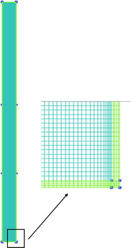
A complete schematic of a TPCT is shown in Figure 1 [46]. The calculation conditions are set based on experimental results. The lengths of the evaporation, adiabatic, and condensation sections are 100, 100, and 150 mm, respectively. The inner diameter is 16.5 mm, the wall thickness is 0.8 mm, and the shell material is aluminum. The working fluid is acetone, and its physical parameters are listed in Table 2 [47]. The liquid filling rate (the ratio of the liquid volume to the total volume of the HP) is 28.6%. The working fluid is dominated by axial and radial flows rather than a swirling flow. Therefore, the computational domain can be simplified to a two-dimensional geometric model to reduce the simulation time [37,48].

Figure 1. Two-dimensional representation of a TPCT [46].

Table 2. Physical properties of acetone [47].

Physical property	Unit	Liquid phase value	Vapor phase value
Density	kg/m^3	748.95	Ideal gas law
Specific heat	J/(kg K)	2229.3	1567.3
Thermal conductivity	W/(m K)	0.14091	0.014033
Dynamic viscosity	kg/(m s)	2.3986 × 10^−4	8.3032 × 10^−6
Molecular mass	kg/kmol	58.0498
Latent heat	kJ/kg	501.42
Surface tension	N/m	0.0188

Fixed-heat-flux conditions (q_in = 17,606 W/m², q_out = −11,737 W/m²) are defined on the external walls of the evaporation and condensation sections to ensure energy balance between heating and cooling. The external walls of the adiabatic section are set as adiabatic conditions. Coupling with a no-slip boundary condition between the inner wall and fluid region is applied to equalize the heat flux of the solid wall and fluid region next to the inner wall. The initial conditions are set as temperature 329 K and pressure 0.1 MPa.

2.2. Governing equations

A description of the numerical model is shown in Figure 2. The black wireframes represent the original solution process, and the red dotted area represents the modified solution process. The blue font represents the dynamic mass transfer time relaxation parameters (β), which are key to the modified model. β must be updated until stable values are obtained.

Figure 2. Description of the modified model solution process.

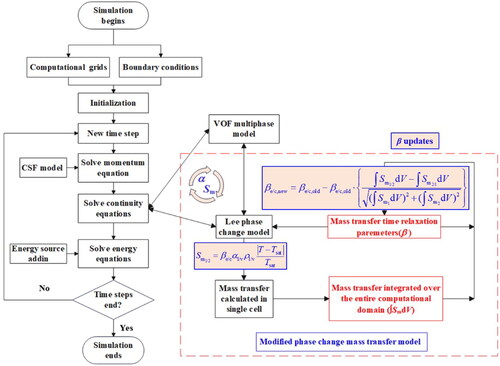
The VOF multiphase flow model is adopted to model the vapor–liquid two-phase flow in a thermosyphon because it can compute the multiphase flows of immiscible fluids and track the motion of their interfaces, as well as the effects of interfacial shear stress and surface tension under gravity [27,49]. In the VOF model, one set of Navier–Stokes equations is solved for the computational domain and used to track the motion of different phases by defining the volume fraction of each phase [50,51]. In a vapor–liquid two-phase flow, α_l and α_v are the volume fractions of the liquid and vapor, respectively, which must sum to unity as given in Eq. (3)(3) $${\alpha }_{\mathrm{l}}+{\alpha }_{\mathrm{v}}=1$$(3) : (3) $${\alpha }_{\mathrm{l}}+{\alpha }_{\mathrm{v}}=1$$(3)

In other words, an empty volume is not allowed in the fluid domain. Therefore, the existence of a particular phase in any control volume can be easily derived from the volume fraction according to the following three cases:

• α_v = 1: The cell is filled with vapor.

• α_v = 0: The cell is filled with liquid.

• 0 < α_v < 1: The cell contains a mixture of liquid and vapor.

The continuity equations for the liquid and vapor phases are defined as follows: (4) $$\frac{\partial ({\alpha }_{\mathrm{l}}{\rho }_{\mathrm{l}})}{\partial t}+\nabla \cdot ({\alpha }_{\mathrm{l}}{\rho }_{\mathrm{l}}\overrightarrow{u})=S_{{\mathrm{m}}_{\mathrm{l}}}$$(4) (5) $$\frac{\partial ({\alpha }_{\mathrm{v}}{\rho }_{\mathrm{v}})}{\partial t}+\nabla \cdot ({\alpha }_{\mathrm{v}}{\rho }_{\mathrm{v}}\overrightarrow{u})=S_{{\mathrm{m}}_{\mathrm{v}}}$$(5) where $S_{{\mathrm{m}}_{\mathrm{l}}}$ and $S_{{\mathrm{m}}_{\mathrm{v}}}$ express the mass source terms of the evaporation and condensation processes, respectively, which are used to calculate the mass transfer of the vapor–liquid two-phase transitions during the evaporation and condensation processes. These expressions are described in a phase change model where ρ_l and ρ_v are the densities of the liquid phase and vapor phase in kg/m³, respectively. $\overrightarrow{u}$ represents the velocity of the vapor–liquid mixed phase in m/s.

The momentum equation is modeled as shown in Eq (6)(6) $$\frac{\partial (\rho \overrightarrow{u})}{\partial t}+\nabla \cdot (\rho \overrightarrow{u}\overrightarrow{u})=\rho \overrightarrow{g}-\nabla p+\nabla \cdot [\mu (\nabla \overrightarrow{u}+\nabla {\overrightarrow{u}}^{\mathrm{T}})]+{\overrightarrow{F}}_{\text{CSF}}$$(6) : (6) $$\frac{\partial (\rho \overrightarrow{u})}{\partial t}+\nabla \cdot (\rho \overrightarrow{u}\overrightarrow{u})=\rho \overrightarrow{g}-\nabla p+\nabla \cdot [\mu (\nabla \overrightarrow{u}+\nabla {\overrightarrow{u}}^{\mathrm{T}})]+{\overrightarrow{F}}_{\text{CSF}}$$(6)

Here, $\overrightarrow{g}$ is the acceleration due to gravity in m/s²; p is the pressure in Pa; and ${\overrightarrow{F}}_{\text{CSF}}$ is the surface tension in N/m³. The CSF model proposed by Brackbill et al. [49] was substituted into the momentum equation to calculate surface tension. The resulting relational expression is as follows [27]: (7) $${\overrightarrow{F}}_{\text{CSF}}=\sigma \frac{\rho \kappa \nabla \alpha }{\frac{1}{2}({\rho }_{\mathrm{l}}+{\rho }_{\mathrm{v}})}$$(7) where ρ is the average density in kg/m³, σ the surface tension coefficient in N/m, and κ the surface curvature in m⁻¹. The expression for the surface curvature κ is written as follows: (8) $$\kappa =\nabla \cdot \frac{\nabla \alpha }{\left|\nabla \alpha \right|}$$(8)

The expression of the energy equation is written as follows: (9) $$\frac{\partial (\rho E)}{\partial t}+\nabla \cdot [\overrightarrow{u}(\rho E+p)=\nabla \cdot (\lambda \nabla T)+S_{\mathrm{E}}$$(9)

Here, E represents the internal energy in J/kg. S_E is the source term of the energy equation and is used to calculate the amount of energy transferred during the evaporation and condensation processes. The expression for the functional relationship between the mass and energy source terms is written as follows: (10) $$S_{\mathrm{E}}=S_{\mathrm{m}}\cdot \text{LH}$$(10)

Here, LH is the latent heat in J/kg.

Heat is transferred inside the metal walls via conduction, and the expression of the energy transport in the metal wall area is written as follows: (11) $${\rho }_{\mathrm{w}}{c}_{\mathrm{w}}\frac{\partial T}{\partial t}={\lambda }_{\mathrm{w}}\left(\frac{{\partial }^{2}T}{\partial x^2}+\frac{{\partial }^{2}T}{\partial y^2}\right)$$(11) where ρ_w is the density of the metal wall, c_w the specific heat, and λ_w the thermal conductivity.

After the volume fraction is calculated, the physical properties φ, including the density ρ, thermal conductivity λ, and dynamic viscosity μ in each grid can be defined based on the volume fraction average method as follows [52]: (12) $$\phi ={\alpha }_{\mathrm{l}}{\phi }_{\mathrm{l}}+{\alpha }_{\mathrm{v}}{\phi }_{\mathrm{v}},\phi \in \left\{\rho ,\lambda ,\mu \right\}$$(12)

The constant-pressure specific heat used to calculate the internal energy E is mass-averaged as follows: (13) $$c_p\text{=}\frac{1}{\rho }\left({\alpha }_{\mathrm{l}}{\rho }_{\mathrm{l}}{c}_{p\text{,l}}+{\alpha }_{\mathrm{v}}{\rho }_{\mathrm{v}}{c}_{p\text{,v}}\right)$$(13)

2.3. Dynamic Lee phase change model

During the vapor–liquid phase transition, the mass and heat transfer models should be considered as source terms, as shown in Figure 2. The objective of this section is to provide a numerical model for estimating the local interphase mass transfer term depending on the local temperature field. The most widely used Lee model is defined as Eqs. (1)(1) $$S_{{\mathrm{m}}_{\mathrm{l}}}={\beta }_{\mathrm{e}}{\alpha }_{\mathrm{l}}{\rho }_{\mathrm{l}}\frac{\left|T-T_{\text{sat}}\right|}{T_{\text{sat}}}\text{for evaporation},T>T_{\text{sat}}$$(1) and (2)(2) $$S_{{\mathrm{m}}_{\mathrm{v}}}=-{\beta }_{\mathrm{c}}{\alpha }_{\mathrm{v}}{\rho }_{\mathrm{v}}\frac{\left|T-T_{\text{sat}}\right|}{T_{\text{sat}}}\text{for condensation},T<T_{\text{sat}}$$(2) [27], where β is the mass transfer time relaxation parameter in s⁻¹, α the phase volume fraction, ρ the density in kg/m³, and T the temperature in K. The subscripts c and v refer to condensation and evaporation, respectively, and sat represents the saturation state. S_m is the mass source term in kg/(m³ s).

The mass transfer calculation process is significantly affected by the mass transfer time relaxation parameters and they cannot be defined as constants. Therefore, instantly updated β_e and β_c values are added to the original Lee model, which must be adjusted by considering both the calculated mass transfer and β_old from the last simulation step. To calculate the total mass transfer between the vapor and liquid in the entire computational region, Eqs. (1)(1) $$S_{{\mathrm{m}}_{\mathrm{l}}}={\beta }_{\mathrm{e}}{\alpha }_{\mathrm{l}}{\rho }_{\mathrm{l}}\frac{\left|T-T_{\text{sat}}\right|}{T_{\text{sat}}}\text{for evaporation},T>T_{\text{sat}}$$(1) and (2)(2) $$S_{{\mathrm{m}}_{\mathrm{v}}}=-{\beta }_{\mathrm{c}}{\alpha }_{\mathrm{v}}{\rho }_{\mathrm{v}}\frac{\left|T-T_{\text{sat}}\right|}{T_{\text{sat}}}\text{for condensation},T<T_{\text{sat}}$$(2) must be integrated over the whole volume. Therefore, β_new can be written as follows: (14) $${\beta }_{\text{e,new}}={\beta }_{\text{e,old}}-{\beta }_{\text{e,old}}\cdot \left\{\frac{{\int }_V{S}_{{\mathrm{m}}_{\mathrm{l}}}\mathrm{d}V-{\int }_V{S}_{{\mathrm{m}}_{\mathrm{v}}}\mathrm{d}V}{\sqrt{{\left({\int }_V{S}_{{\mathrm{m}}_{\mathrm{l}}}\mathrm{d}V\right)}^2+{\left({\int }_V{S}_{{\mathrm{m}}_{\mathrm{v}}}\mathrm{d}V\right)}^2}}\right\}$$(14) (15) $${\beta }_{\text{c,new}}={\beta }_{\text{c,old}}-{\beta }_{\text{c,old}}\cdot \left\{\frac{{\int }_V{S}_{{\mathrm{m}}_{\mathrm{v}}}\mathrm{d}V-{\int }_V{S}_{{\mathrm{m}}_{\mathrm{l}}}\mathrm{d}V}{\sqrt{{\left({\int }_V{S}_{{\mathrm{m}}_{\mathrm{l}}}\mathrm{d}V\right)}^2+{\left({\int }_V{S}_{{\mathrm{m}}_{\mathrm{v}}}\mathrm{d}V\right)}^2}}\right\}$$(15) where ${\int }_V{S}_{{\mathrm{m}}_{\mathrm{l}}}\mathrm{d}V$ and ${\int }_V{S}_{{\mathrm{m}}_{\mathrm{v}}}\mathrm{d}V$ are the total mass transfers during the evaporation and condensation processes, respectively. Their values are obtained using volume integration. Considering the stability of the numerical calculations, the denominators of the iterative formula are written in the form described above.

2.4. Solution strategy and numerical approach

In the VOF model, the liquid is considered the primary phase, and the vapor is the secondary phase. A fixed time step of 5 × 10⁻⁵ s is used in the transient simulation process, which is controlled by a global Courant number which is less than 1.0. The SIMPLE algorithm is used for pressure–velocity coupling, which is a second-order upwind numerical scheme for momentum and energy equation discretization. Geo-reconstruction and PRESTO! are used for the discretization of the volume fraction and pressure interpolation scheme, respectively. The numerical calculations are considered to be converged when the scaled residuals of the mass and velocity are less than 10⁻⁶ and that of the energy is less than 10⁻⁹.

2.5. Grid independence test and numerical model validation

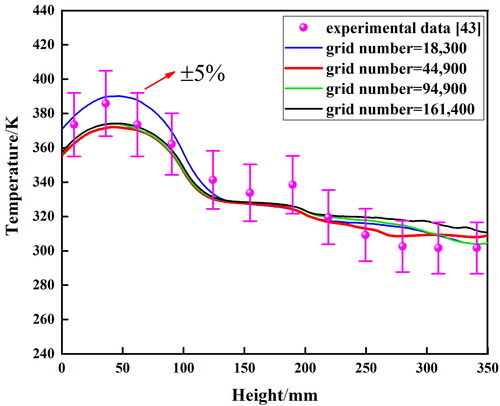
Structured grids employed in the computational domain are shown in Figure 3, and the grids are refined with a growth rate of 1.2 near the inner walls, where phase changes occur. Four different numbers of grids are tested to ensure that the numerical results are independent of the number of cells, which is determined by comparing the temperature distributions outside the walls. Therefore, the total number of cells for the TPCT is set at 44,900.

Figure 3. Grid independence test and validation of temperature distribution outside the walls.

The developed numerical model is validated using experimental data from Solomon et al. [46]. The relative error is less than 5%, indicating good agreement between the numerical results and experimental data. The results of the grid independence test and the numerical model validation are shown in Figure 4.

Figure 4. Grid independence test and validation of temperature distribution outside the walls.

3. Results and discussion

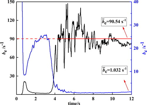
3.1. Variation of the instantly updated mass transfer time relaxation parameters

The transient mass transfer time relaxation parameters calculated using the modified model are shown in Figure 5. In the first 4 s, as shown in Figure 5, β changes significantly from the initial values. After t = 4 s, β_c gradually becomes sufficiently stable. β_e still oscillates over time, but the amplitude of the oscillations becomes increasingly small and eventually stabilizes. After t = 4 s, the time–average values of β_e and β_c are 90.54 and 1.032 s⁻¹, respectively.

Figure 5. Instantly updated mass transfer time relaxation parameters calculated by the modified model.

3.2. Two-phase flow and phase change process details

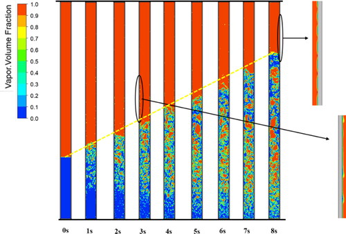
The phase change process details for the modified model (initial values of β_e and β_c are 10 and 200 s⁻¹, respectively) and the original model (β_e = 10 s⁻¹, β_c = 1000 s⁻¹) are shown in Figures 6 and 7, respectively. They both exhibit a nucleate boiling phenomenon in which bubbles appear in the boiling liquid pool at the evaporator. In addition, the newly formed microbubbles near the inner wall of the evaporator merged into larger bubbles. In the first 4 s in Figure 6, the vapor-phase volume fraction changes significantly because the iterative calculation is not yet stable. After t = 4 s, the iterative calculation gradually stabilizes. The liquid levels also tend to stabilize. However, the liquid level calculated by the original model continuously increases approximately linearly (yellow line in Figure 7) and does not stabilize until the calculation diverges at t = 8 s. The amount of mass transfer from vapor to liquid is greater than that from liquid to vapor, which causes the liquid level to increase significantly. A continuous condensation film forms inside the condenser in Figure 6, whereas the liquid film is intermittent in Figure 7. The liquid film in the former is thinner than that in the latter. When the liquid film calculated by using the original model is first formed, it is intermittent. However, as the falling water clings to the wall under the force of gravity, the discontinuous liquid film slowly converges into large droplets.

Figure 6. Contours of the vapor volume fraction calculated by the modified model.

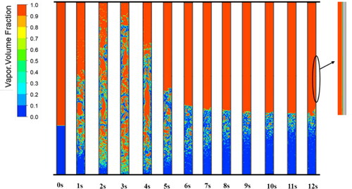
Figure 7. Contours of the vapor volume fraction calculated by the original model.

3.3. Temperature distribution and thermal resistance

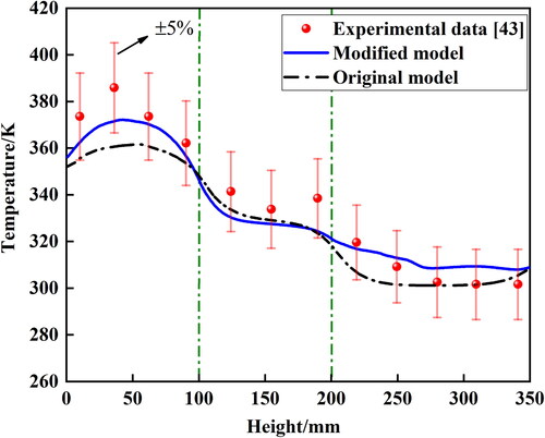
The temperature distribution outside the walls is shown in Figure 8. The results of both the modified and original models exhibit good agreement with the experimental data [46]. However, the temperatures of evaporation and condensation calculated by the modified model contain less error than the original model. The continuous liquid film in the modified model is unfavorable for heat transfer in the condensation section. When a continuous liquid film exists, the thermal conduction process through the liquid film weakens the vapor condensation. Therefore, the temperature outside the condensation section of the original model is lower than that of the modified model and experimental data.

Figure 8. Comparison of temperature distributions outside the walls.

The thermal resistances of the evaporation, condensation sections, and the total thermal resistances are calculated as follows: (16) $$R_e=\frac{T_{\mathrm{e}}-T_{\mathrm{v}}}{Q}$$(16) (17) $$R_{\mathrm{c}}=\frac{T_{\mathrm{v}}-T_{\mathrm{c}}}{Q}$$(17) where T_e, T_c, and T_v are the wall temperature of evaporation section, the wall temperature of condensation section, and the vapor temperature, respectively.

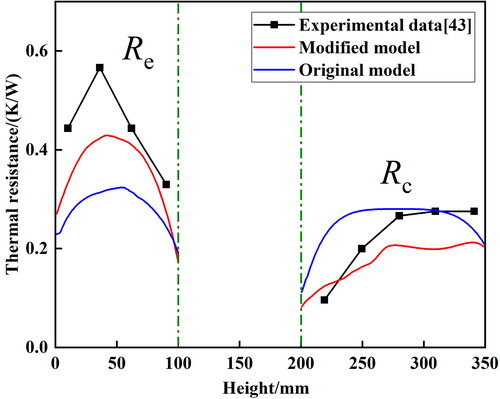
The results of thermal resistances using the modified and original models are shown in Figure 9. The error of thermal resistance in evaporation section (R_e) calculated by the modified model is 7.5–25.3%, while that of the original model is 25.8–44.6%. For the condensation section, the error of the thermal resistance (R_c) calculated by the modified model is 18.4–30.4%, while that of the original model is 0.49–137.5%. Compared with the original model, the maximum thermal resistance errors in evaporation section and condensation section of the modified model are reduced by 19.3% and 107.1%, respectively. Besides, the error ranges of the modified model are also lower than those of the original model.

Figure 9. Thermal resistance calculated by the modified and original models.

4. Conclusions

A dynamic Lee phase change model coupled with the VOF model and CSF model is developed to predict the heat transfer characteristics and phase change processes in a TPCT. Dynamic adjustment of the mass transfer time relaxation parameters for the Lee phase change model is realized and β_e and β_c become stabilized eventually to $\overline{{\beta }_{\mathrm{e}}}$ = 90.54 s⁻¹ and $\overline{{\beta }_{\mathrm{c}}}$ = 1.032 s⁻¹, respectively. The reliability and accuracy of the prediction of the temperature distribution and thermal resistance are validated. Compared with the original model, the maximum thermal resistance errors in evaporation section and condensation section of the modified model are reduced by 19.3% and 107.1%, respectively.

Nomenclature
cp	=	specific heat (J/kg K)
E	=	internal energy (J/kg)
${\overrightarrow{F}}_{\text{CSF}}$	=	surface tension (N/m3)
LH	=	latent heat (J/kg)
p	=	pressure (Pa)
R	=	thermal resistance (K/W)
SE	=	source term in the energy conservation equation (J/m3 s)
Sm	=	source term in the mass conservation equation (kg/m3 s)
T	=	temperature (K)
t	=	time (s)
$\overrightarrow{u}$	=	velocity vector (m/s)

Greek symbols
α	=	phase volume fraction
β	=	mass transfer time relaxation parameter (1/s)
κ	=	surface curvature (1/m)
λ	=	thermal conductivity (W/m K)
μ	=	dynamic viscosity (kg/m s)
ρ	=	density (kg/m3)
σ	=	surface tension coefficient (N/m)
$\nabla$	=	gradient
$\nabla \cdot$	=	divergence

Subscripts
c	=	condensation
e	=	evaporation
l	=	liquid
new	=	new value
old	=	old value
sat	=	saturation
v	=	vapor
w	=	wall

Disclosure statement

The authors declare no conflict of interest in this paper.

Additional information

Funding

This study is supported by National Natural Science Foundation of China [52106082] and Heilongjiang Province Science and Technology Major Project [CN, 2020ZX10A03].

References

- J. Cao et al., “A review on independent and integrated/coupled two-phase loop thermosyphons,” Appl. Energy, vol. 280, pp. 115885, Dec. 2020. DOI: 10.1016/j.apenergy.2020.115885.
- R. Wen, W. Liu, X. Ma, and R. Yang, “Coupling droplets/bubbles with a liquid film for enhancing phase-change heat transfer,” iScience, vol. 24, no. 6, pp. 102531, Jun. 2021. DOI: 10.1016/j.isci.2021.102531.
- V. Guichet and H. Jouhara, “Condensation, evaporation and boiling of falling films in wickless heat pipes (two-phase closed thermosyphons): a critical review of correlations,” Int. J. Thermofluids, vol. 1–2, pp. 100001, Feb. 2020. DOI: 10.1016/j.ijft.2019.100001.
- B. Fadhl, L. C. Wrobel, and H. Jouhara, “Numerical modelling of the temperature distribution in a two-phase closed thermosyphon,” Appl. Therm. Eng., vol. 60, no. 1–2, pp. 122–131, Oct. 2013. DOI: 10.1016/j.applthermaleng.2013.06.044.
- H. Jouhara and H. Ezzuddin, “Thermal performance characteristics of a wraparound loop heat pipe (WLHP) charged with R134A,” Energy, vol. 61, no. 1, pp. 128–138, Nov. 2013. DOI: 10.1016/j.energy.2012.10.016.
- S. Kloczko and A. Faghri, “Thermal performance and flow characteristics of two-phase loop thermosyphons,” Numer. Heat Transf., Part A, vol. 77, no. 7, pp. 683–701, Jan. 2020. DOI: 10.1080/10407782.2020.1714342.
- Y.-C. Weng, H.-P. Cho, C.-C. Chang, and S.-L. Chen, “Heat pipe with PCM for electronic cooling,” Appl. Energy, vol. 88, no. 5, pp. 1825–1833, May 2011. DOI: 10.1016/j.apenergy.2010.12.004.
- L. L. Vasiliev, “State-of-the-art on heat pipe technology in the former Soviet Union,” Appl. Therm. Eng., vol. 18, no. 7, pp. 507–551, Jul. 1998. DOI: 10.1016/S1359-4311(97)00005-7.
- D. Redpath, “Thermosyphon heat-pipe evacuated tube solar water heaters for northern maritime climates,” Sol. Energy, vol. 86, no. 2, pp. 705–715, Feb. 2012. DOI: 10.1016/j.solener.2011.11.015.
- L. L. Vasiliev, “Heat pipes in modern heat exchangers,” Appl. Therm. Eng., vol. 25, no. 1, pp. 1–19, Jan. 2005. DOI: 10.1016/j.applthermaleng.2003.12.004.
- S. H. Noie-Baghban and G. R. Majideian, “Waste heat recovery using heat pipe heat exchanger (HPHE) for surgery rooms in hospitals,” Appl. Therm. Eng., vol. 20, no. 14, pp. 1271–1282, Oct. 2000. DOI: 10.1016/S1359-4311(99)00092-7.
- H. Jouhara and A. Robinson, “An experimental study of small-diameter wickless heat pipes operating in the temperature range 200 °C to 450 °C,” Heat Transf. Eng., vol. 30, no. 13, pp. 1041–1048, Jul. 2009. DOI: 10.1080/01457630902921113.
- C. Zhang, S. Wu, F. Yao, and D. Sun, “Numerical study on vapor–liquid phase change in an enclosed narrow space,” Numer. Heat Transf., Part A, vol. 77, no. 2, pp. 199–214, Jan. 2020. DOI: 10.1080/10407782.2019.1685821.
- C. R. Kharangate and I. Mudawar, “Review of computational studies on boiling and condensation,” Int. J. Heat Mass Transf., vol. 108, no. Part A, pp. 1164–1196, May 2017. DOI: 10.1016/j.ijheatmasstransfer.2016.12.065.
- G. Y. Soh, G. H. Yeoh, and V. Timchenko, “An algorithm to calculate interfacial area for multiphase mass transfer through the volume-of-fluid method,” Int. J. Heat Mass Transf., vol. 100, pp. 573–581, Sep. 2016. DOI: 10.1016/j.ijheatmasstransfer.2016.05.006.
- G. Y. Soh, G. H. Yeoh, and V. Timchenko, “Improved volume-of-fluid (VOF) model for predictions of velocity fields and droplet lengths in microchannels,” Flow Meas. Instrum., vol. 51, pp. 105–115, Oct. 2016. DOI: 10.1016/j.flowmeasinst.2016.09.004.
- J. Choi and Y. Zhang, “Numerical simulation of oscillatory flow and heat transfer in pulsating heat pipes with multi-turns using OpenFOAM,” Numer. Heat Transf., Part A, vol. 77, no. 8, pp. 761–781, Feb. 2020. DOI: 10.1080/10407782.2020.1717202.
- F. He, W. Dong, and J. Wang, “Modeling and numerical investigation of transient two-phase flow with liquid phase change in porous media,” Nanomaterials (Basel), vol. 11, no. 1, pp. 183–196, Jan. 2021. DOI: 10.3390/nano11010183.
- Y. You, G. Wang, C. Guo, and H. Jiang, “Study on mass transfer time relaxation parameter of indirect evaporative cooler considering primary air condensation,” Appl. Therm. Eng., vol. 181, pp. 115958, Nov. 2020. DOI: 10.1016/j.applthermaleng.2020.115958.
- Z. Cao, D. Sun, J. Wei, and B. Yu, “Boiling heat transfer by using the VOSET method based on unstructured grids,” Chin. Sci. Bull., vol. 65, no. 17, pp. 1723–1733, Jun. 2020. DOI: 10.1360/TB-2019-0573.
- Q. Shen, D. Sun, S. Su, N. Zhang, and T. Jin, “Development of heat and mass transfer model for condensation,” Int. Commun. Heat Mass Transf., vol. 84, pp. 35–40, May 2017. DOI: 10.1016/j.icheatmasstransfer.2017.03.009.
- D. Sun, J. Xu, and Q. Chen, “Modeling of the evaporation and condensation phase-change problems with FLUENT,” Numer. Heat Transf., Part B, vol. 66, no. 4, pp. 326–342, Aug. 2014. DOI: 10.1080/10407790.2014.915681.
- Y. Zai, Y. Qiao, C. Song, H. Tao, and Y. Li, “Numerical analysis of flow characteristics and bubble behavior inside a two-phase closed thermosyphon under various temperature difference” Numer. Heat Transf., Part A, pp. 1–18, Jan. 2023. DOI: 10.1080/10407782.2023.2178561.
- Y. Liu, Z. Li, Y. Jiang, C. Guo, and D. Tang, “Analysis of the two-phase flow, heat transfer, and instability characteristics in a loop thermosyphon,” Numer. Heat Transf., Part A, vol. 79, no. 9, pp. 656–680, May 2021. DOI: 10.1080/10407782.2021.1882820.
- C. W. Hirt and B. D. Nichols, “Volume of fluid (VOF) method for the dynamics of free boundaries,” J. Comput. Phys., vol. 39, no. 1, pp. 201–225, Jan. 1981. DOI: 10.1016/0021-9991(81)90145-5.
- M. Huang, L. Wu, and B. Chen, “A piecewise linear interface-capturing volume-of-fluid method based on unstructured grids,” Numer. Heat Transf., Part B, vol. 61, pp. 412–437, Jun. 2012. DOI: 10.1080/10407790.2012.672818.
- S. C. K. De Schepper, G. J. Heynderickx, and G. B. Marin, “Modeling the evaporation of a hydrocarbon feedstock in the convection section of a steam cracker,” Comput. Chem. Eng., vol. 33, no. 1, pp. 122–132, Jan. 2009. DOI: 10.1016/j.compchemeng.2008.07.013.
- Y. W. Kuang, W. Wang, R. Zhuan, and C. C. Yi, “Simulation of boiling flow in evaporator of separate type heat pipe with low heat flux,” Ann. Nucl. Energy, vol. 75, pp. 158–167, Jan. 2015. DOI: 10.1016/j.anucene.2014.08.008.
- H. Yao, C. Yue, Y. Wang, H. Chen, and Y. Zhu, “Numerical investigation of the heat and mass transfer performance of a two-phase closed thermosiphon based on a modified CFD model,” Case Stud. Therm. Eng., vol. 26, pp. 101155, Aug. 2021. DOI: 10.1016/j.csite.2021.101155.
- Z. Xu, Y. Zhang, B. Li, and J. Huang, “Modeling the phase change process for a two-phase closed thermosyphon by considering transient mass transfer time relaxation parameter,” Int. J. Heat Mass Transf., vol. 101, pp. 614–619, Oct. 2016. DOI: 10.1016/j.ijheatmasstransfer.2016.05.075.
- S. Abadi, W. A. Davies, P. Hrnjak, and J. P. Meyer, “Numerical study of steam condensation inside a long inclined flattened channel,” Int. J. Heat Mass Transf., vol. 134, pp. 450–467, May 2019. DOI: 10.1016/j.ijheatmasstransfer.2019.01.063.
- B. Fadhl, L. C. Wrobel, and H. Jouhara, “CFD modelling of a two-phase closed thermosyphon charged with R134a and R404a,” Appl. Therm. Eng., vol. 78, pp. 482–490, Mar. 2015. DOI: 10.1016/j.applthermaleng.2014.12.062.
- A. Alizadehdakhel, M. Rahimi, and A. A. Alsairafi, “CFD modeling of flow and heat transfer in a thermosyphon,” Int. Commun. Heat Mass Transf., vol. 37, no. 3, pp. 312–318, Mar. 2010. DOI: 10.1016/j.icheatmasstransfer.2009.09.002.
- A. A. Alammar, R. K. Al-Dadah, and S. M. Mahmoud, “Numerical investigation of effect of fill ratio and inclination angle on a thermosiphon heat pipe thermal performance,” Appl. Therm. Eng., vol. 108, pp. 1055–1065, Sep. 2016. DOI: 10.1016/j.applthermaleng.2016.07.163.
- Y. Wang et al., “CFD simulation of an intermediate temperature, two-phase loop thermosiphon for use as a linear solar receiver,” Appl. Energy, vol. 207, pp. 36–44, Dec. 2017. DOI: 10.1016/j.apenergy.2017.05.168.
- Y. Wang, X. Wang, H. Chen, R. A. Taylor, and Y. Zhu, “A combined CFD/visualized investigation of two-phase heat and mass transfer inside a horizontal loop thermosiphon,” Int. J. Heat Mass Transf., vol. 112, pp. 607–619, Sep. 2017. DOI: 10.1016/j.ijheatmasstransfer.2017.04.132.
- X. Wang, H. Yao, J. Li, Y. Wang, and Y. Zhu, “Experimental and numerical investigation on heat transfer characteristics of ammonia thermosyhpons at shallow geothermal temperature,” Int. J. Heat Mass Transf., vol. 136, pp. 1147–1159, Jun. 2019. DOI: 10.1016/j.ijheatmasstransfer.2019.03.080.
- X. Wang, Y. Zhu, and Y. Wang, “Development of pressure-based phase change model for CFD modelling of heat pipes,” Int. J. Heat Mass Transf., vol. 145, pp. 118763, Dec. 2019. DOI: 10.1016/j.ijheatmasstransfer.2019.118763.
- Y. Kim, J. Choi, S. Kim, and Y. Zhang, “Effects of mass transfer time relaxation parameters on condensation in a thermosyphon,” J. Mech. Sci. Technol., vol. 29, no. 12, pp. 5497–5505, Dec. 2015. DOI: 10.1007/s12206-015-1151-5.
- K. Kafeel and A. Turan, “Simulation of the response of a thermosyphon under pulsed heat input conditions,” Int. J. Therm. Sci., vol. 80, pp. 33–40, Jun. 2014. DOI: 10.1016/j.ijthermalsci.2014.01.020.
- Z. Xu, Y. Zhang, B. Li, C.-C. Wang, and Y. Li, “The influences of the inclination angle and evaporator wettability on the heat performance of a thermosyphon by simulation and experiment,” Int. J. Heat Mass Transf., vol. 116, pp. 675–684, Jan. 2018. DOI: 10.1016/j.ijheatmasstransfer.2017.09.028.
- Z. Xu, Y. Zhang, B. Li, C.-C. Wang, and Q. Ma, “Heat performances of a thermosyphon as affected by evaporator wettability and filling ratio,” Appl. Therm. Eng., vol. 129, pp. 665–673, Jan. 2018. DOI: 10.1016/j.applthermaleng.2017.10.073.
- H. Liu, J. Tang, L. Sun, Z. Mo, and G. Xie, “An assessment and analysis of phase change models for the simulation of vapor bubble condensation,” Int. J. Heat Mass Transf., vol. 157, pp. 119924, Aug. 2020. DOI: 10.1016/j.ijheatmasstransfer.2020.119924.
- G. Chen, T. Nie, and X. Yan, “An explicit expression of the empirical factor in a widely used phase change model,” Int. J. Heat Mass Transf., vol. 150, pp. 119279, Apr. 2020. DOI: 10.1016/j.ijheatmasstransfer.2019.119279.
- Z. Tan, Z. Cao, W. Chu, and Q. Wang, “Dynamic correction on condensation time relaxation coefficient of Lee model based on mass conservation mechanism,” Int. Commun. Heat Mass Transf., vol. 142, pp. 106621, Mar. 2023. DOI: 10.1016/j.icheatmasstransfer.2023.106621.
- A. Brusly Solomon, A. Mathew, K. Ramachandran, B. C. Pillai, and V. K. Karthikeyan, “Thermal performance of anodized two phase closed thermosyphon (TPCT),” Exp. Therm. Fluid Sci., vol. 48, pp. 49–57, Jul. 2013. DOI: 10.1016/j.expthermflusci.2013.02.007.
- M. L. Huber, E. W. Lemmon, and M. D. McLinden, NIST Standard Reference Database 23: Reference Fluid Thermodynamics and Transport Properties-REFPROP, in: Vol. Version 9.1, National Institute of Standards and Technology, Standard Reference Data Program, 2013.
- S.-D. Fertahi, T. Bouhal, Y. Agrouaz, T. Kousksou, T. El Rhafiki, and Y. Zeraouli, “Performance optimization of a two-phase closed thermosyphon through CFD numerical simulations,” Appl. Therm. Eng., vol. 128, pp. 551–563, Jan. 2018. DOI: 10.1016/j.applthermaleng.2017.09.049.
- J. U. Brackbill, D. B. Kothe, and C. Zemach, “A continuum method for modeling surface tension,” J. Comput. Phys., vol. 100, no. 2, pp. 335–354, Jun. 1992. DOI: 10.1016/0021-9991(92)90240-Y.
- R. Marek and J. Straub, “Analysis of the evaporation coefficient and the condensation coefficient of water,” Int. J. Heat Mass Transf., vol. 44, no. 1, pp. 39–53, Jan. 2001. DOI: 10.1016/S0017-9310(00)00086-7.
- F. Dong, Z. Wang, T. Cao, and J. Ni, “A novel interphase mass transfer model toward the VOF simulation of subcooled flow boiling,” Numer. Heat Transf., Part A, vol. 76, no. 4, pp. 220–231, Aug. 2019. DOI: 10.1080/10407782.2019.1627838.
- Y. Lin et al., “A numerical study of slug bubble growth during flow boiling in a diverging microchannel,” Numer. Heat Transf., Part A, vol. 80, no. 7, pp. 356–367, Oct. 2021. DOI: 10.1080/10407782.2021.1947093.