Minimizing the Maximum Expected Sample Size in Two-Stage Phase II Clinical Trials with Continuous Outcomes

Abstract

Two-stage designs are commonly used for Phase II trials. Optimal two-stage designs have the lowest expected sample size for a specific treatment effect, for example, the null value, but can perform poorly if the true treatment effect differs. Here we introduce a design for continuous treatment responses that minimizes the maximum expected sample size across all possible treatment effects. The proposed design performs well for a wider range of treatment effects and so is useful for Phase II trials. We compare the design to a previously used optimal design and show it has superior expected sample size properties.

Key Words:

• Minimax design
• Optimal design
• Two-stage designs

1. INTRODUCTION

A randomized controlled Phase II clinical trial is used to assess whether an intervention has a significant treatment effect compared to a control treatment. For a single-stage design, a group of patients is recruited and randomized between arms, with the overall treatment effect assessed. There are ethical and statistical advantages to using a two-stage design. Such designs allow stopping the trial early for lack of treatment effect (futility), or for sufficient evidence of treatment effect (efficacy). Stopping early for futility means fewer patients are exposed to an intervention that is probably ineffective and may have side effects. Stopping for efficacy means that a potentially useful intervention progresses through the drug development progress more quickly. Lee and Feng (2005) reviewed recent study designs in oncology trials and found that 45% used two-stage designs, although many did not allow stopping for efficacy.

Much work has been done on group sequential methods, where a trial has several interim analyses, and the trial can stop for futility and/or efficacy after any stage. Although these designs reduce the expected number of patients required to detect a significant treatment effect, there are a couple of disadvantages. First, it may not be convenient to stop a study multiple times for interim analyses, especially in trials where the endpoint takes a long time to measure. Second, we may be interested in choosing the sample sizes per group and thresholds at which the trial stops to minimize the expected sample size. An optimal design is one that has the lowest expected sample size for a specific treatment effect, subject to it having the correct type I error and power under a prespecified clinically relevant difference (CRD). Trials with several stages have many possible parameters, and thus are difficult to optimize.

A compromise is a two-stage design that has fewer parameters to optimize over, thus reducing the computational burden, and provides many of the benefits of a multi-stage design. A two-stage design also requires just one interim analysis. Optimal two-stage designs have been considered for binary outcomes by Simon (1989), and for continuous outcomes by Whitehead et al. (2009). Designs in each of these papers were designed to be optimal under a specific treatment effect.

We aim to show in this paper that these designs, especially ones optimal under the null of no treatment advantage, can have very poor properties when the true treatment effect differs from that which the design is optimized for. When the trial allows stopping for either futility or efficacy, each design has a treatment effect that gives the highest expected sample size. We call this the “worst-case scenario” treatment effect, and propose a new type of design that has the lowest expected sample size under the worst-case scenario treatment effect. We call this design the δ-minimax design, to avoid confusion with the minimax design that minimizes the total sample size.

We first discuss how to find the worst-case scenario treatment effect, and some issues involved in finding the optimal design. We then show null-optimal, CRD-optimal, and δ-minimax designs for a variety of design parameters, and compare their performance for a range of possible treatment effects. Lastly, we compare the δ-minimax design to an optimal two-stage design from Whitehead et al. (2009). The δ-minimax design has a 5% lower maximum expected sample size, an 8% lower expected sample size under the null treatment effect, and a 3% lower expected sample size under the CRD.

2. TWO-STAGE DESIGNS FOR BINARY AND CONTINUOUS TREATMENT RESPONSES

A lot of work on optimal two-stage designs has been done in the context of binary responses. Often there will be a latent continuous treatment response, which is dichotomized to give the binary response. An example is the RECIST criteria used in classifying a cancer patient's response to treatment, which is a function of the change in tumor size (Eisenhauer et al., 2009). Reclassifying a continuous response to a binary response loses information (Farewell et al., 2004; Karrison et al., 2007), but is still commonly done.

The Simon two-stage design (Simon, 1989) is commonly used for binary responses. Simon proposed the optimal design as the one with lowest expected sample size under the null hypothesis. Also proposed was the minimax design, which has the lowest combined first- and second-stage sample size. Simon's design has been the basis of many subsequent designs. It has been adapted to stop for efficacy, for example, by Jones and Holmgren (2007). The optimal and minimax designs are special cases of admissible designs, discussed by Jung et al. (2004).

A design based around the continuous treatment response is described by Whitehead et al. (2009). Again, n ₁ and n ₂ are the sample sizes in the first and second stages, respectively. The response is assumed to be normally distributed, and a normalizing transformation of the p-value from a one-sided t-test is used as the test statistic after the first stage. If the test statistic is below a threshold, f, the trial is stopped for futility, and if it is above e ₁, it is stopped for efficacy. If the trial continues, the null hypothesis is rejected if the test statistic for the combined n ₁ + n ₂ patients is above e ₂. The design also can be adapted to allow n ₂ to change, conditional on the estimated standard deviation of treatment effect in the first stage.

Several other two-stage designs (Li et al., 2002; Proscan and Hunsberger, 1995; Posch and Bauer, 1999) have an adaptive second-stage sample size conditional on the first-stage test statistic. Although this allows considerable flexibility in carrying out a trial, it may be desirable for trial organizers, participants, and grant committees to know the second stage sample size in advance, even if it results in a slight increase in expected sample size.

3. OPTIMAL TWO-STAGE DESIGNS FOR CONTINUOUS TREATMENT RESPONSES

In this paper we assume that an individual's response to treatment (possibly after correcting for other covariates, e.g., in a linear regression) is distributed as for the control treatment, and for the tested treatment, where and are unknown. We assume that σ _T  = σ _C  = σ. If δ = δ _T  − δ _C is the true difference in treatment effect, we assume that the null and alternative hypotheses being tested are:

Generally a design will be sought that has type I error α, and type II error of β when δ = δ*, and σ = σ*, where δ* is a clinically relevant difference that would be desirable to detect, and σ* is the value of the standard deviation used to design the trial which may be the estimated treatment response standard deviation from previous trials or a pilot study. A continuous two-stage design can be parameterized by (n ₁, n ₂, f, e ₁, e ₂, R), where:

1.	n 1 is the number of patients recruited to the control arm in the first stage.
2.	n 2 is the number of patients recruited to the control arm in the second stage, if the second stage occurs.
3.	R is the allocation ratio, the ratio of number of patients in the case arm to the number in the control arm. We assume for the rest of the paper that R = 1, that is, the trial is balanced.
4.	f is the lower threshold for the first-stage test statistic, below which the trial stops for futility.
5.	e 1 is the upper threshold for the first-stage test statistic, above which the trial stops for efficacy and the null is rejected.
6.	e 2 is the threshold for the joint first- and second-stage test statistic, above which the null hypothesis is rejected.

The two-stage trial that we use consists of testing the treatment responses of the first-stage patients with a two-sample t-test, giving a statistic T ₁. If T ₁ is less than f, the trial is stopped for futility; if it is greater than e ₁, the trial stops for efficacy, and H ₀ is rejected; otherwise the trial continues to the second stage. The treatment responses of patients recruited to the second stage are tested using a two-sample t-test, giving statistic T ₂. If is above e ₂, the null hypothesis is rejected. This form of the test statistic used at the second stage results in easier computation of the distribution conditional on the first-stage test statistic than one that uses the pooled T-test. For large sample sizes, both forms should give a similar result. For details on how to calculate the overall probability of rejecting H ₀, see, for example, Jennison and Turnbull (2000).

The trial will be designed such that the probability of rejecting the null hypothesis under the null is less than or equal to α, and the probability of rejecting the null hypothesis for δ ≥ δ* is greater than or equal to 1 − β. If a two-stage design meets the constraints on (α, β), we refer to it as a feasible design.

Given a feasible two-stage design parameterized by (n ₁, n ₂, f, e ₁, e ₂), two quantities of interest are the probability of early termination (PET(δ)), and the expected sample size, 𝔼(N | δ). PET(δ) is the probability of the trial being stopped after the first stage, due to either futility or efficacy, and is equal to:

and 𝔼(N | δ) depends on n ₁, n ₂, PET(δ) as follows:

Note that PET depends on the true value of δ. To calculate 𝔼(N | δ) under different values of δ, one can calculate PET(δ) from equation (1), using that T ₁ is distributed as a noncentral t random variable with noncentrality parameter , and degrees of freedom 2n ₁ − 2. 𝔼(N | δ) can then be found from PET(δ) using equation (2). To simplify the notation, we refer to PET(δ) and 𝔼(N | δ) as PET and 𝔼(N) henceforth.

As the true δ increases, the trial is more likely to stop for efficacy, but less likely to stop for futility. This leads to PET decreasing to a minimum point, and then increasing as δ increases. 𝔼(N) has the reverse relationship, since a lower PET results in a higher 𝔼(N).

For each design, (n ₁, n ₂, f, e ₁, e ₂), there exists a δ that minimizes PET, and thus maximizes 𝔼(N). We call this value the worst-case scenario treatment effect, and label it . Minimizing PET is equivalent to maximizing:

with respect to δ, where f _{T 1} is the pdf of the non central t distribution. This can be found through a simple interval bisection technique. Although this adds some computation to finding the δ-minimax design, it is not much extra since it involves evaluating the CDF of the one-dimensional t distribution. Most of the computation time in finding two-stage designs is taken up in finding the overall type I error and power, which involves two-dimensional integrals.

The null-optimal design is the feasible design that minimizes 𝔼(N | δ = 0), the CRD-optimal design is the one that minimizes 𝔼(N | δ = δ*), and the δ-minimax design is the one that minimizes . The latter is slightly misleading notation, since depends on the design parameters, whereas the other two quantities do not depend on the design. To be more precise, if F is the set of all feasible designs, with d _i an individual feasible design, the δ-minimax design is the design d such that

In this way the only assumptions we make about δ are those we must do to power the trial. If we choose a design that optimizes the expected sample size under a specific value of δ (as the null and CRD optimal designs do), then if the true δ is different, the design we choose will have a large expected sample size. The δ-minimax design minimizes the impact of deviations from the assumptions necessary to design the trial.

4. TECHNICAL CONSIDERATIONS FOR FINDING OPTIMAL DESIGNS

With five design parameters to search over, and nonlinear constraints on type I error and power to meet, finding an optimal design is a complicated optimization problem. One approach is to minimize 𝔼(N | δ) subject to constraints. Finding an analytical expression for the derivatives of 𝔼(N | δ) with respect to each of the parameters is difficult, but a numerical estimate can be used instead. Two complications are that the final n ₁ and n ₂ parameters must be integers, and the type I and II error constraints must be met. In addition, the space of possible designs contains many local minima (with respect to 𝔼(N | δ)). These problems seem to imply that a deterministic minimization method is not feasible to use.

Instead we used a straightforward grid search to look for the optimal designs. This examines each combination of (n ₁, n ₂, f, e ₁, e ₂), and keeps a record of the design with lowest expected sample size (under the relevant δ) that meets the type I and II error constraints. A few constraints can be used to reduce the number of designs searched over:

1.	e 1 must be greater than or equal to the 1 − α quantile of the first-stage test statistic under δ = 0, otherwise the type I error probability of the two-stage design is greater than α.
2.	f must be less than or equal to the β quantile of the first-stage test statistic under δ = δ*, otherwise the type II error probability of the two-stage design is greater than β.
3.	e 1 is assumed to be less than or equal to 5. Allowing values greater than 5 has a minimal effect on the properties of the designs found, but means the grid search takes longer.
4.	f is assumed to be greater than or equal to −1, for a similar reason to the preceding one.
5.	From empirical data, n 1 appears to be greater than or equal to one quarter of the required sample size for a feasible one-stage design, so this is used as a constraint.
6.	n 1 must be less than the lowest 𝔼(N | δ) found so far, since 𝔼(N | δ) is always at least n 1.

The process of finding the optimal designs works by increasing n ₁ and cycling through feasible values of f, e ₁ in increments of 0.1. For each combination of (n ₁, f, e ₁), the second-stage parameters (n ₂, e ₂) are found such that the design is feasible, and n ₂ is the minimum of all feasible designs with first-stage parameters (n ₁, f, e ₁) (thus reducing 𝔼(N | δ)). After the optimal design from the coarse grid given earlier is found, the grid is tightened, and the area near to the current optimal design is searched.

For cases where is large, and thus the required sample size is large, this process will be extremely time-consuming. For the rest of this paper, we have limited the preceding ratio to be less than or equal to 10. For Phase II trials, the assumed ratio would generally be lower than this.

5. RESULTS

5.1. Optimal Designs and Their Relative Performance

For this first section we assume the true σ is equal to the σ* used to design the study, but explore how deviations from this assumption affect the expected sample size and power later on.

We found the null-optimal, CRD-optimal, and δ-minimax designs for three standard ombinations of type I and II error probabilities: (α, β) ∈ {(0.05, 0.1), (0.1, 0.1), (0.05, 0.2)}. These combinations, which had previously been studied by Simon (1989), allow us to compare the relative performance of the designs as the type I error probability is increased, and as the type II error probability is increased. For each design, δ* was taken to be 1, with σ* ∈ {1, 2, 5, 10}. These values are arbitrary, but reflect a range of possible trial sizes. σ = 10 results in a trial much larger than any that would be done at Phase II, but we feel that it is instructive to examine how the designs perform for large sample sizes. Note that the designs depend only on the ratio , so the optimal designs for different values of δ* can easily be found from the following results.

Table 1 gives the design parameters of the different designs for (α, β) = (0.05, 0.1). For comparative purposes, it also gives the sample size per arm required for the single stage design. Figure 1 is a line graph showing the expected total sample size of the different designs for δ ∈ [0, 2δ*].

Figure 1 Plot of expected sample sizes of each optimal design against true mean treatment response, δ, for (α, β) = (0.05, 0.1). (Color figure available online.).

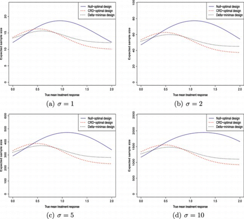
Table 1 Optimal designs and their expected sample sizes when δ = 0, δ*, or for (α, β) = (0.05, 0.1)

							𝔼(N) under
Design	n 1	n 2	f	e 1	e 2		H 0	CRD
σ = 1
Null-optimal design	8	13	0.5	3.51	1.62	0.95	12.04	18.68	18.70
CRD-optimal design	10	11	0.36	1.98	1.95	0.52	13.65	14.01	16.22
δ-minimax design	12	8	0.86	2.10	1.76	0.60	13.44	14.42	15.60
Single-stage design	18	–	–	1.69	–	–	18	18	18
σ = 2
Null-optimal design	31	52	0.5	3.82	1.55	1.08	47.13	77.17	77.37
CRD-optimal design	37	43	0.22	1.91	1.88	0.49	53.48	53.14	62.65
δ-minimax design	45	35	0.81	1.95	1.74	0.58	51.44	54.72	60.02
Single-stage design	70	–	–	1.66	–	–	70	70	70
σ = 5
Null-optimal design	189	315	0.45	4.40	1.55	1.10	291.88	480.30	488.29
CRD-optimal design	226	267	0.13	1.88	1.87	0.48	337.60	327.37	390.93
δ-minimax design	277	209	0.75	1.95	1.73	0.57	319.031	337.35	371.23
Single-stage design	429	–	–	1.65	–	–	429	429	429
σ = 10
Null-optimal design	762	1238	0.45	4.5	1.55	1.27	1166.10	1910.73	1946.46
CRD-optimal design	918	1057	0.18	1.87	1.87	0.48	1338.45	1306.71	1554.02
δ-minimax design	1101	846	0.75	1.95	1.72	0.57	1271.09	1346.95	1482.85
Single-stage design	1714	–	–	1.65	–	–	1714	1714	1714

Table 1 shows some general features of each design. The null-optimal design has the lowest first-stage sample size, together with a positive value of f, and a large value of e ₁. This is because decreasing e ₁ does not reduce 𝔼(N | δ = 0) as much as increasing f does. Although this results in a smaller 𝔼(N) when δ = 0, it drastically affects the expected sample size when δ is larger.

The CRD-optimal design has a smaller value of e ₁ which results in a lower 𝔼(N | δ = δ*). On the other hand, the design tends to have a smaller f. This smaller f means that 𝔼(N) is somewhat higher than the null-optimal design when δ is near to 0.

The δ-minimax design generally has a larger f than the null-optimal design, and a value of e ₁ close to that of the CRD-optimal design. In order to control the increased type II error probability that the higher f causes, a larger n ₁ is needed. Thus, although f, and therefore PET, under the null is higher, the δ-minimax design still has a larger 𝔼(N) under the null than the null-optimal design due to the larger sample size in the first stage.

Also given in Table 1 are the values of , the treatment effect that gives the highest expected sample size, for the different designs. As Fig. 1 shows, is highest for the null-optimal designs, smaller for the δ-minimax designs, and smallest in the CRD-optimal designs. As the trial size increases, increases in the null-optimal designs, and decreases in the CRD-optimal and δ-minimax designs.

Figure 1 shows that for low values of , the CRD-optimal design is almost identical to the δ-minimax design. As the ratio increases, the two designs become more separated, with maximum expected sample size being noticeably lower under the δ-minimax design. Graphs 1(c) and 1(d) appear to be roughly the same shape, but with different y-axis scales. This would indicate that as σ increases, the relative shapes of the designs converge, and only the scale increases.

Figure 1 also shows that the null-optimal design is clearly best for low values of δ, but very poor for values of δ close to the CRD. As δ increases, the probability of stopping for efficacy will converge toward 1. Thus, 𝔼(N) for the null-optimal design will be superior for very large values of δ also. The point at which the null-optimal design stops being optimal appears to decrease as σ increases due to the decrease in PET. In Fig. 1(a) it is 0.275, but in Fig. 1(d), it has reduced to 0.242.

Figure 1 shows that the relative performance of 𝔼(N) of each optimal design appears to converge as σ increases. This implies that the ratios of the maximum expected sample size under the CRD-optimal and null-optimal design respective to the maximum under the δ-minimax design will also converge. Table 2 shows both of these ratios as increases. The maximum expected sample size ratio of the CRD-optimal and δ-minimax design increases to just over 1.05, and then falls slightly for σ = 10. This could mean that the designs in Table 1 are close to being the optimal designs, but not quite exactly. For the true globally optimal design, one would expect the ratio to increase with σ, and converge. The null-optimal design performs worse, with the maximum expected sample size larger. The ratio increases with σ, with a slight fall for σ = 10, due to the same reasons as previously. The ratio converges to a value just above 1.31.

Table 2 Ratio of maximum E(N) under CRD-optimal and designs to maximum E(N) under δ-minimax design

	Ratio of from CRD-optimal and δ-minimax designs	Ratio of from null-optimal and δ-minimax designs
1	1.039	1.199
2	1.044	1.289
5	1.053	1.315
10	1.048	1.313

Table 1 also includes the (unique) single-stage design that gives the required type I and II error probabilities. The table shows that the expected sample size of the CRD-optimal and δ-minimax designs are always lower than the single-stage design (but not for the null-optimal design for δ near to the CRD). On the other hand, n ₁ + n ₂ is always higher than the sample size required for the single-stage design. This was not the case for Simon two-stage designs, which occasionally produced designs where n ₁ + n ₂ was lower than the single-stage sample size (Simon, 1989). This is likely to be a feature of the discrete nature of the Simon design, which does not translate to the continuous designs we examine here.

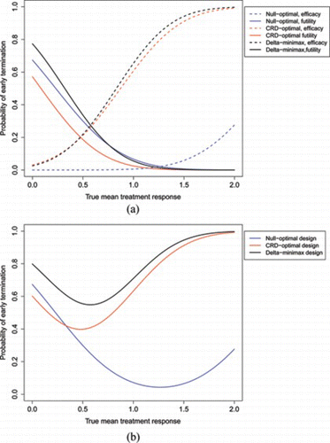
Due to the correspondence between 𝔼(N) and PET, examining how PET varies with δ may be instructive. Figure 2 shows two different graphs. The first shows the probability of stopping for futility and efficacy separately for each design. The second shows the overall PET for each design. As expected, the δ-minimax actually has a larger probability of stopping for futility than the null-optimal design when δ is near the null. Interestingly, it also has a larger probability of stopping for efficacy, in comparison to the CRD-optimal design, when δ is close to the CRD. Figure 2(b) shows that the δ-minimax design has the largest PET for every value of δ considered. These factors are all desirable for a two-stage design, even if a larger first-stage sample size is needed for them to be true.

Figure 2 Plots comparing probability of stopping after first stage for different values of δ for null-optimal (blue), CRD-optimal (red), and δ-minimax (black) designs. (α, β) = (0.05, 0.1), σ = 10. (a) Probability of stopping for efficacy (dashed) and futility (solid) after stage 1 for three optimal designs. (b) Total probability of early termination.

Tables 3 and 4, together with Figs. 3 and 4, give the corresponding results using different type I and type II error probabilities. Table 3 and Fig. 3 give results for (α, β) = (0.05, 0.2), with the other two giving results for (α, β) = (0.1, 0.1). These plots allow comparison of the relative performance of the designs if (1) the permitted type II error probability is increased and (2) the permitted type I error probability is increased.

Figure 3 Plot of expected sample sizes against true treatment effect, (α, β) = (0.05, 0.2). (Color figure available online.).

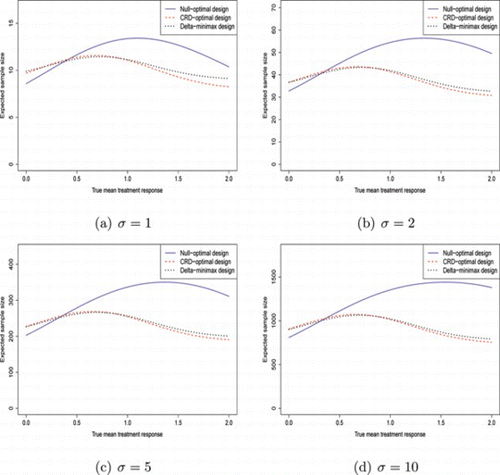
Figure 4 Plot of expected sample sizes against true treatment effect, (α, β) = (0.1, 0.1). (Color figure available online.).

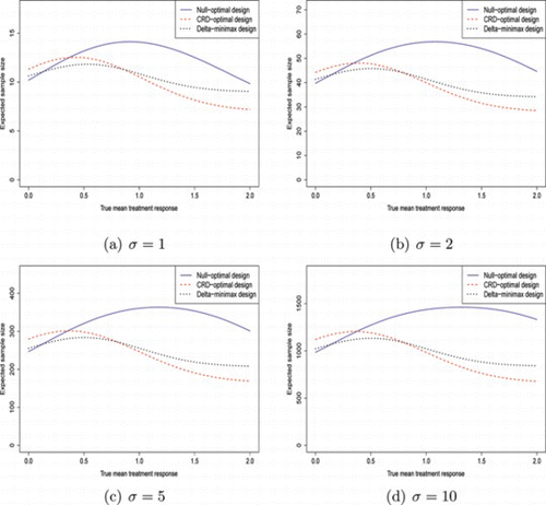
Table 3 Optimal designs and their expected sample sizes for (α, β) = (0.05, 0.2)

							𝔼(N) under
Design	n 1	n 2	f	e 1	e 2		H 0	CRD
σ = 1
Null-optimal design	5	11	0.47	3.25	1.66	1.10	8.58	13.37	13.42
CRD-optimal design	8	7	0.65	2.11	1.86	0.68	9.69	11.07	11.58
δ-minimax design	9	6	0.99	2.12	1.76	0.72	9.90	11.13	11.45
Single-stage design	14	–	–	1.71	–	–	14	14	14
σ = 2
Null-optimal design	20	41	0.5	3.84	1.54	1.33	32.76	54.46	56.37
CRD-optimal design	30	28	0.63	1.95	1.80	0.66	36.69	41.40	43.61
δ-minimax design	32	25	0.83	2.05	1.69	0.72	36.60	41.88	43.33
Single-stage design	51	–	–	1.66	–	–	51	51	51
σ = 5
Null-optimal design	125	249	0.49	3.85	1.52	1.36	202.79	336.58	350.19
CRD-optimal design	186	170	0.61	1.92	1.78	0.65	227.38	254.34	268.69
δ-minimax design	197	157	0.8	1.98	1.70	0.70	226.53	256.51	266.65
Single-stage design	310	–	–	1.65	–	–	310	310	310
σ = 10
Null-optimal design	505	987	0.5	4.41	1.52	1.54	809.63	1353.28	1441.46
CRD-optimal design	738	688	0.6	1.91	1.78	0.65	907.37	1014.75	1073.29
δ-minimax design	777	641	0.78	1.97	1.70	0.69	900.91	1022.27	1064.15
Single-stage design	1238	–	–	1.65	–	–	1238	1238	1238

Table 4 Optimal designs and their expected sample sizes for (α, β) = (0.1, 0.1)

							𝔼(N) under
Design	n 1	n 2	f	e 1	e 2		H 0	CRD
σ = 1
Null-optimal design	6	10	0.2	3.19	1.26	0.91	10.20	14.09	14.13
CRD-optimal design	7	10	0	1.60	1.65	0.42	11.32	10.54	12.54
δ-minimax design	9	7	0.58	1.68	1.40	0.53	10.63	10.85	11.83
Single-stage design	14	–	–	1.31	–	–	14	14	14
σ = 2
Null-optimal design	25	35	0.2	3.72	1.21	1.08	39.75	56.73	56.84
CRD-optimal design	28	35	−0.07	1.54	1.55	0.39	44.19	39.97	48.08
δ-minimax design	34	26	0.43	1.64	1.37	0.50	41.35	41.44	45.78
Single-stage design	53	–	–	1.29	–	–	53	53	53
σ = 5
Null-optimal design	156	222	0.23	3.93	1.19	1.17	246.83	360.59	363.38
CRD-optimal design	165	222	−0.2	1.53	1.54	0.37	279.59	246.40	301.14
δ-minimax design	207	172	0.43	1.61	1.37	0.50	255.18	255.58	283.63
Single-stage design	329	–	–	1.28	–	–	329	329	329
σ = 10
Null-optimal design	651	840	0.26	4.49	1.19	1.31	984.87	1436.39	1471.76
CRD-optimal design	663	880	−0.21	1.53	1.54	0.36	1120.61	983.70	1204.63
δ-minimax design	837	681	0.45	1.6	1.37	0.50	1021.90	1022.64	1132.95
Single-stage design	1315	–	–	1.28	–	–	1315	1315	1315

If the type II error probability is increased to 0.2, there appears to be a much smaller difference between the CRD-optimal design and the δ-minimax design. This is because it allows f to be increased in the CRD-optimal design. On the other hand, f for the δ-minimax design was already high, so increasing the type II error does not increase it much further. Thus, it seems for α = 0.05 and β = 0.2, there is little advantage in using the δ-minimax design over that from using the CRD-optimal design. However, both are significantly better than the null-optimal design when δ is near to the CRD. As σ increases, the δ at which the δ-minimax design has a lower expected sample size than the null-optimal design decreases from 0.38 to 0.32.

For (α, β) = (0.1, 0.1), the pattern looks different. First, the CRD-optimal design and δ-minimax design are more distinct than they were for (α, β) = (0.05, 0.2). Under the null, 𝔼(N) of the δ-minimax design is very close to the null-optimal design, whereas when δ=δ*, 𝔼(N) of the δ-minimax design is slightly further away from the 𝔼(N) of the CRD-optimal design. This implies that compared to (α, β) = (0.05, 0.1), increasing the type I error causes the δ-minimax design to be slightly closer in performance under the null to the null-optimal design, whereas increasing the type II error causes it to be closer to the CRD-optimal design across a wider variety of treatment responses.

5.2. Comparison to Whitehead's Optimal Continuous Design

Earlier we discussed the paper by Whitehead et al. (2009) in which a two-stage trial was designed for a Phase II trial of placebo against a novel compound for the control of diabetic neuropathic pain. Although we have used different test statistics in this paper, the overall procedure is very similar.

Whitehead et al. simplified the computation by fixing the total number of patients in the first stage to be 90 (i.e., n ₁ = 45 when the allocation ratio is 1), and f to be 0. This reduces the dimension of the search space to three, which does speed up the searching significantly. Six designs were found that covered a range of (α, β) combinations and different allocation ratios. δ* was set to be 1, with σ* = 2.3. We compare design 1 in Table 1 of the Whitehead paper to two δ-minimax designs we found. For that design, (α, β) = (0.025, 0.2), the allocation ratio is equal to 1, and the design was optimized under the null of δ = 0. The first δ-minimax design we found constrained n ₁ to be equal to 45, to make it more comparable to Whitehead's design; the second did not have a constraint on n ₁.

Table 5 shows the design parameters for each of the three designs, and the resulting 𝔼(N) under δ = 0, δ = 0.5, and δ = 1 (values that were given in Table 1 of Whitehead et al.).

Table 5 Comparison of design parameters and resulting expected sample sizes between (1) the first design in Table 1 in Whitehead et al. (2009), (2) the δ-minimax design with n ₁ constrained to be 45, and (3) the δ-minimax design with n ₁ unconstrained

	Whitehead's	δ-minimax n 1 = 45	δ-minimax n 1 unconstrained
n 1 per arm	45	45	54
f	0	0.850	1.110
e 1	2.730	2.367	2.303
n 2 per arm	39	52	42
e 2	1.977	2.023	2.018
𝔼(N | δ = 0)	128.75	109.75	118.45
𝔼(N | δ = 0.5)	152.71	139.73	140.38
𝔼(N | δ = 1)	146.79	142.28	140.71

Both δ-minimax designs perform better than Whitehead's design for each of the three values of δ examined. Under the null, the expected number of patients when δ = 0 is around 20 less using the constrained δ-minimax, and 10 less using the unconstrained one. This shows how important the f parameter is for the null optimal design, with f = 0 providing a 50% chance of early termination under the null, but as shown earlier, the null-optimal design has a PET under the null that converges to around 70% as tends to ∞.

Whitehead et al. do not provide a plot summarizing the expected sample size at each δ point, so we used the design parameters from Table 5 and applied them using the two-stage design procedure discussed in this paper. This appears to result in slightly lower than specified expected sample sizes. For example, under δ = 0, the expected sample size of Whitehead's design was 128.7 instead of 128.75 given in the paper. This difference is extremely small, so we feel comfortable in comparing the designs in this way. Figure 5 shows the expected sample size of each of the three designs for every δ value between 0 and 2δ*.

Figure 5 Comparison of expected sample sizes, as the true δ varies, between the three designs in Table 5. (Color figure available online.).

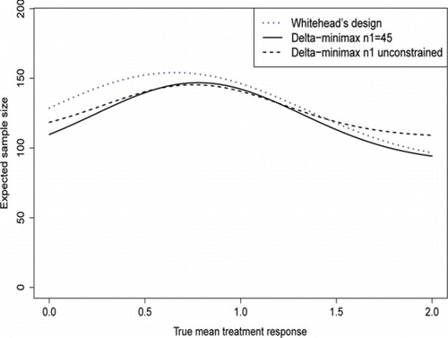
From the plot in Fig. 5, both δ-minimax designs perform better in terms of 𝔼(N) for δ values between δ = 0 and δ = δ*. The constrained δ-minimax design appears to be the best one, with a substantial drop in 𝔼(N) for values of δ near the null or greater than δ*; it does slightly worse at values of δ near .

Whitehead's design performs better than the unconstrained δ-minimax design when δ is greater than around 1.5δ*. This is because of its lower first-stage sample size, which the expected sample size converges to as δ increases. Although this is a disadvantage of the unconstrained δ-minimax design, it does mean that a more precise estimate of δ is given, which allows a subsequent Phase III trial to be designed more efficiently.

All of the designs just described control the type I error, but not the power, when the true value of σ differs from 2.3. Table 6 shows the power as σ varies. There is not a great deal of difference between the three designs, with all suffering a loss of power as σ increases. The loss of power is slightly higher for Whitehead's design when σ > 2.3. On the other hand, for σ values smaller than 2.3, the power gain is slightly higher with Whitehead's design. This indicates that the two δ-minimax designs are very slightly more robust to deviations of σ from σ*.

Table 6 Power of Whitehead's design, constrained δ-minimax design, and unconstrained δ-minimax design for values of σ different from the assumed value of 2.3

	Power
σ	Whitehead's	δ-minimax n 1 = 45	δ-minimax n 1 unconstrained
1.4	0.995	0.992	0.994
1.8	0.945	0.942	0.944
2.4	0.761	0.767	0.766
2.8	0.628	0.637	0.636
3.2	0.517	0.525	0.524

6. DISCUSSION

In this paper we have introduced the δ-minimax design to controlled two-stage Phase II trials with continuous outcomes. The δ-minimax design minimizes the maximum possible expected sample size under all possible treatment effects. A paper by Shuster (2002) uses this criterion on uncontrolled binary trials, although there it was named “minimax”. To avoid confusion with the design that minimizes the maximum sample size, we name the criterion δ-minimax. This is the first paper to apply such a criterion to controlled trials with continuous treatment responses and to compare it to other optimal designs for a full range of possible treatment effects. Previous work has tended to define optimality as optimal under the null hypothesis, for example, in Simon (1989). This appears to be a poor choice unless:

1.	The null hypothesis is highly likely to be true, in which case why is the trial being performed?
2.	There is a strong clinical reason to use it, for example, an expensive or toxic drug that should be stopped early if it is having no effect.

The δ-minimax design can be seen as minimizing the impact of the “worse-case scenario” occurring. Not only does it have this advantage, but it appears to perform well for a range of other values of δ too. The only situation when it has the highest expected sample size is when δ is much higher than the clinically relevant difference, δ*. Generally δ* is somewhat optimistic, so this will seldom be the case. The design is no more difficult to find than other optimal designs. We implemented the grid-search technique using C, with code available on request.

If the type II error probability, β, is allowed to be higher, the differences between the δ-minimax design and the CRD-optimal design are far less pronounced. For β = 0.2, there was very little to choose between them. Both still appear to be a more suitable choice than the null-optimal design.

In the results section, we showed that the probability of early termination is always higher using the δ-minimax design than using the other two optimal designs. For values of δ close to the null, it had a higher probability of stopping for futility than the null-optimal design, and for values close to the CRD, it had a higher probability of stopping for efficacy than the CRD-optimal design. It still loses out slightly in terms of 𝔼(N) in both cases because of the higher first-stage sample size.

Although the expected sample size is higher than that of the CRD-optimal design when δ is near to the CRD, this may be not be a completely bad thing. Since the treatment is shown to be effective, a larger Phase III trial would probably be planned, and the extra information from the larger first-stage sample may come in handy to plan it.

The δ-minimax designs have larger first-stage and maximum sample sizes than the other optimal designs. This larger sample size allows PET to be higher for all treatment effects. In section 5.2 we showed that limiting the first-stage sample size reduces the maximum sample size without losing too much in terms of maximum expected sample size. Designs that balance the maximum expected sample size and maximum sample size may be desirable and worth further research.

Designs here have all been based on a controlled Phase II trial. The theoretical distributions underlying them can easily be extended to the case of an uncontrolled trial, a type commonly used for cancer trials. The relative performance of the designs is the same for the uncontrolled, but each design needs roughly a quarter of the total sample size.

The idea of optimal two-stage designs can be extended to more than two stages. This would have the advantage of giving lower expected sample sizes. Methods from group sequential trials have considered optimality under the null, but do not tend to optimize the design under all possible parameters (i.e., sample size per stage, futility and efficacy parameters for each stage). For a design with many stages, it is a considerable computational challenge to find the optimal design, with the grid search becoming infeasible to use. Stochastic search methods such as simulated annealing could be used, and may provide faster searches.

Overall, the δ-minimax design has desirable properties, and may be a better choice for designing two-stage Phase II trials than ones that assume a specific treatment effect to optimize under.

ACKNOWLEDGMENTS

JMSW and APM are funded by the UK Medical Research Council (grant codes G08008600 and U.1052.00.014). We thank Dr Thomas Jaki for his helpful comments on the article. We also thank the two anonymous reviewers for their helpful and constructive comments.

REFERENCES

- Eales , J. D. , Jennison , C. ( 1995 ). Optimal two-sided group sequential tests . Sequential Analysis 14 : 273 – 286 .
- Eisenhauer , E. , Therasse , P. , et al. ( 2009 ). New response evaluation criteria in solid tumours: Revised RECIST guideline (version 1.1) . European Journal of Cancer 45 : 228 – 247 .
- Farewell , V. , Tom , B. , Royston , P. ( 2004 ). The impact of dichotomization on the efficiency of testing for an interaction effect in exponential family models . Journal of the American Statistical Association 99 : 822 – 831 .
- Jennison , C. , Turnbull , B. ( 2000 ). Group Sequential Methods with Applications to Clinical Trials . Boca Raton , FL : Chapman and Hall .
- Jones , C. , Holmgren , E. ( 2007 ). An adaptive simon two-stage designs for phase 2 studies of targeted therapies . Contemporary Clinical Trials 28 : 654 – 661 .
- Jung , S. , Lee , T. , Kim , K. , George , S. ( 2004 ). Admissible two-stage designs for Phase II cancer clinical trials . Statistics in Medicine 23 : 561 – 569 .
- Karrison , T. , Maitland , M. , Stadler , W. , Ratain , M. ( 2007 ). Design of Phase II cancer trials using a continuous endpoint of change in tumour size: Application to a study of sorafenib and erlotinib in non-small-cell lung cancer . JNCI 99 : 1455 – 1461 .
- Lee , J. , Feng , L. ( 2005 ). Randomized Phase II designs in cancer clinical trials: current status and future directions . Journal of Clinical Oncology 23 : 4450 – 4457 .
- Li , G. , Shih , W. , Xie , T. , Lu , J. ( 2002 ). A sample size adjustment procedure for clinical trials based on conditional power . Biostatistics 3 : 277 – 287 .
- Posch , M. , Bauer , P. ( 1999 ). Adaptive two stage designs and the conditional error function . Biometrical Journal 6 : 689 – 696 .
- Proscan , M. , Hunsberger , S. (1995). Designed extension of studies based on conditional power. Biometrics 51:1315–1324.
- Shuster , J. ( 2002 ). Optimal two-stage designs for single-arm Phase II cancer trials . Journal of Biopharmaceutical Statistics 22 : 39 – 51 .
- Simon , R. ( 1989 ). Optimal two-stage designs for Phase II clinical trials . Controlled Clinical Trials 10 : 1 – 10 .
- Whitehead , J. , Valdes-Marquez , E. , Lissmats , A. ( 2009 ). A simple two-stage design for quantitative responses with application to a study in diabetic neuropathic pain . Pharmaceutical Statistics 8 : 125 – 135 .