
 ?Mathematical formulae have been encoded as MathML and are displayed in this HTML version using MathJax in order to improve their display. Uncheck the box to turn MathJax off. This feature requires Javascript. Click on a formula to zoom.
Abstract
The Birch and Swinnerton-Dyer conjecture has been numerically verified for the Jacobians of 32 modular hyperelliptic curves of genus 2 by Flynn, Leprévost, Schaefer, Stein, Stoll and Wetherell, using modular methods. In the calculation of the real period, there is a slight inaccuracy, which might give problems for curves with non-reduced components in the special fiber of their Néron model. In this present article, we explain how the real period can be computed, and how the verification has been extended to many more hyperelliptic curves, some of genus 3, 4, and 5, without using modular methods.
1. Introduction
In [CitationBirch and Swinnerton-Dyer 65], Birch and Swinnerton-Dyer first stated their famous conjecture, based on computations with elliptic curves. Later, in [CitationTate 66], Tate generalized the conjecture to abelian varieties of higher dimension.
Conjecture 1
(BSD, [CitationHindry and Silverman 2000, Conj. F.4.1.6, p. 462]). Let be an abelian variety of dimension d and algebraic rank r. Let L(A, s) be its L-function,
its dual, RA its regulator,
its Tate-Shafarevich group and PA its period. For each prime p, let cp be the Tamagawa number of A at p. Then L(A, s) has a zero of order r at s = 1 and
Remark 2.
In Tate’s original version, [CitationTate 66], the period, Tamagawa numbers and discriminant are put in the normalization of the L-function.
Tate stated the conjecture for abelian varieties over number fields. However, in [CitationMilne 72], Milne proved that the conjecture is compatible with Weil restriction, so BSD holds for all abelian varieties overall number fields if and only if it holds for all abelian varieties over
Due to work of Kolyvagin [CitationKolyvagin 89, CitationKolyvagin 91] and others, a weak version of BSD has been proven for elliptic curves over with analytic rank at most 1. More precisely, we know that in these cases the algebraic rank equals the analytic rank. On the other hand, on the numerical side, in [CitationFlynn et al. 01] Flynn et al. numerically verified BSD for the Jacobians of 32 hyperelliptic curves of genus 2 with small conductor, using modular methods for their calculations.
There is, however, a slight inaccuracy in [CitationFlynn et al. 01]. In the calculation of the real period, calculations seem to be done inside the sheaf of relative differentials, while they should be done inside the canonical sheaf. For curves whose Néron model has non-reduced fibers, this could cause a problem. For the curves considered, it did not seem to invalidate the final results.
The goal of this article is twofold. On the one hand, we will give a more explicit algorithm to compute the real period, or more specifically, a Néron differential, along with the theoretical foundations that are needed for this. On the other hand, we will present how we extended the numerical verification of BSD to the Jacobians of many more hyperelliptic curves of genus 2, 3, 4, and 5 without using modular methods. As far as the author is aware, this is the first time BSD has been numerically verified for the Jacobians of curves of genus 3, 4, and 5.
We did not compute, however, the order of Moreover, the verification is only provable up to squares. That is, all terms but
are computed, of which some are only provably correct up to squares. Then it is verified that the conjectural order of
as predicted by the conjecture, up to a certain high precision, is a rational square or two times a rational square, in accordance with the criteria described in [CitationPoonen and Stoll 99, Sect. 8, pp. 1125–1126].
The structure of this article is as follows. First we present our verification results. Then we discuss the computation of the real period and the theoretical background needed. Then in the last part we briefly discuss the computation of the other terms in the BSD formula.
2. Results
For the Jacobians of the curves listed below, we numerically verified BSD in the following sense. We numerically determined the algebraic and analytic rank, the special value of the L-function, the regulator (provably only up to squares), the real period, the Tamagawa numbers, and the size of the torsion subgroup of the Jacobian, assuming some conjectures mentioned below. Then the BSD formula was used to calculate a conjectural order for and it was verified that it is a rational square (which it should be according to the criteria in [CitationPoonen and Stoll 99]).
In practice this meant that the conjectural order for was less than
away from an integer. Moreover, for all but one of the curves of genus 2, this conjectural order was actually equal to 1.000000000.
The conjectural results that we assume to hold for the verification include the analytic continuation, and the correctness of the functional equation of the L-function (see [CitationHindry and Silverman 2000, Conj. F.4.1.5, p. 461]). When we computed the analytic rank, we did this by numerically checking whether the L-function and its derivatives up to certain order, vanish at 1. Even though this does not prove that these functions vanish, we do assume this to be true. Moreover, we assume the correctness of Ogg’s formula for the computation of the 2-part of the conductor (for more details, see Remark 15). In a certain sense, one could say that our verification also provides evidence for these conjectures.
List of curves
All elliptic curves of the form
with
All hyperelliptic curves from [CitationFlynn et al. 01], comparing it with the outcomes given in that article.
All 300 hyperelliptic curves C of genus 2, of the form
All six hyperelliptic curves of genus 3, of the form
with and
that is, we checked BSD, up to squares, for
and, in order to have an example of rank 1, the curve
As far as we are aware these are the first examples of curves of genus 3 for which BSD has been numerically verified. These were the invariants we found:
Table
For the torsion and regulator, points were searched up to a certain height on the Jacobian. This maximum search height is considerably smaller than the height given by the various height bounds in the literature. It is possible that the size of the torsion subgroups and the regulator is incorrect, but this would only cause a rational square error factor for the value of
The curve
The curve
Remark 3.
It could be the case that some of these curves have isomorphic (or isogenous) Jacobians. Then we actually verified BSD two times for the same abelian variety. In the verification process, we did not check for this.
Remark 4.
Even though for all our curves the verification went well, it should be remarked that problems are to be expected when trying to verify BSD for Jacobians of curves with higher discriminant (or rather, higher conductor). The computation of the L-function takes much longer in these cases. Also the computation of the regulator will be harder, as the heights of the points involved might increase, in particular in case the Mordell-Weil rank is higher.
It should be feasible to carry out the verification for more of the small examples from Harrison’s list, [CitationHarrison 18] of genus 4, as long as the maximum bad prime is small enough. We also tried the verification for some more examples of genus 5, but in these cases the computation of the special value of the L-function was taking hours and the computation of the regular model sometimes did not seem to finish in reasonable time.
3. Theory of differentials
Let be a smooth, geometrically irreducible, projective curve of genus g over
Let
be its Jacobian. The goal of this section is to define the period of J, and to describe a way to compute it in the case C is hyperelliptic. We will be following the algorithm described in [CitationFlynn et al. 01, sect. 3.5].
First we will discuss both the theoretical considerations that are needed for this algorithm.
Throughout the section p will be a prime and S will be the scheme The generic point of S is called η and the special point p.
3.1. Preliminaries
First, for completeness, we will recall the following definition.
Definition 5
([CitationBosch et al. 90, p. 166]). A (relative) curve over S is a normal, proper, flat S-scheme, such that for all
the fiber
is of pure dimension 1. A model of C over S is a relative curve
over S together with an isomorphism
Remark 6.
Without the normality assumption, the special fiber of a curve over S could have embedded components. In order to be able to use the results from [CitationBosch et al. 90], which have been partially derived from [CitationRaynaud 70], it is necessary to not have embedded components.
Let be a Néron model of J over S, and let
be a regular model of C. Assume that the geometric multiplicities of the irreducible components of
in
have greatest common divisor 1.
Theorem 7
([CitationBosch et al. 90, Thm. 4(b), sect. 9.5, p. 267]). Under these conditions, is a separated scheme and
coincides with the identity component of
From [CitationRaynaud 70, Prop. 5.2, p. 46], it now follows that is cohomologically flat, which we will need for the next part.
3.2. Differentials of Jacobian and regular model
A classical theorem (see e.g. [CitationMilne 86, Prop. 2.2, p. 172]) relates the differentials on the Jacobian of a smooth curve over a field with the differentials on the curve itself. We will generalize this to and
Definition 8
([CitationLiu 02, Def. 4.7, sect. 6.4.2, p. 239]). Let Y/T be a quasi-projective locally noetherian scheme. Let be an immersion into a smooth scheme Z/T. Then the canonical sheaf of Y/T is defined to be the
-module
where
is the sheaf of ideals defining Y in an open
containing Y as closed subset. This is independent of the choice of Z and i, see loc. cit.
The following lemma generalizes the aforementioned theorem.
Lemma 9.
There are canonical isomorphisms of -modules
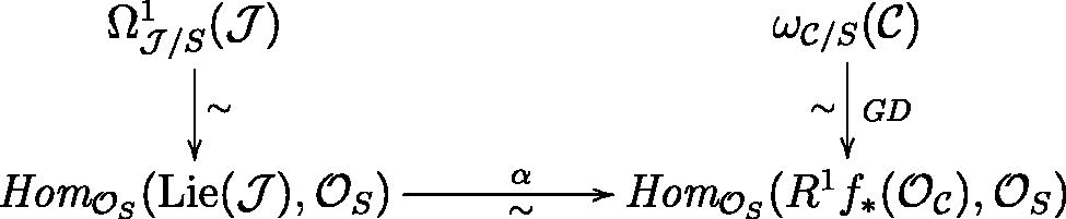
Proof.
The right hand isomorphism is given by Grothendieck duality, see [CitationLiu 02, Sect. 6.4.3, p. 243]. The bottom isomorphism, α, is from [CitationBosch et al. 90, Thm. 8.4.1, p. 231] (here we use that is cohomologically flat). Getting the left hand isomorphism is a little bit more involved.
First remark that global differentials on an abelian variety are translation invariant. As the image of J is dense in also the differentials in
are translation invariant. Combining this with [CitationBosch et al. 90, Prop. 4.2.1, p. 100], we get
(3–1)
(3–1)
where
is the unit section. Now, by [CitationLiu 02, Prop. 6.1.24, p. 217], we get an exact sequence of
-modules
where
is the ideal of the schematic image of e inside
As both
and
and hence
are locally free of rank g (as
is regular), we get that the kernel of
is torsion. As
is torsion-free in our case, and hence the locally free module
is torsion-free, we find a canonical isomorphism of
-modules
which gives, by taking global sections and composing with Equation (1–3), the construction of the left hand isomorphism in the diagram. □
Remark 10.
Under the natural identifications and
the isomorphism
in the lemma above is compatible with the aforementioned classical isomorphism
3.3. Algorithm for the real period
Suppose that are such that, for every prime p, they form a
-basis of
under the identification
In other words, cf. Lemma 9, suppose that
correspond to generators of
where
is a Néron model of J over
Moreover, let
form a symplectic basis for the homology. Then the real period can be defined as follows.
Definition 11.
The real period of J is the covolume of the lattice
where
for
Now suppose that we are working with a hyperelliptic curve given by for some
Then, due to Van Wamelen there is a procedure in Magma to compute a symplectic basis of
as mentioned before, and the integrals
for all
and
In order to compute the real period, we only need to find a basis as above in terms of the differentials
For our purpose, the calculation can be done for each prime p separately. Fortunately for us, due to Donnely, Magma also has an algorithm to compute explicit equations for a regular model
of C over S. It will represent
by giving charts, each of which is a relative complete intersection. The following lemma explicitly gives the isomorphism
that we need to compute whether a certain differential is vanishing or having a pole on one of the components of the special fiber (Step 5 and 6 in Algorithm Citation13).
Lemma 12.
Let be regular, flat, and of relative dimension 1 over
. Suppose that
is a relative complete intersection inside
, given by equations
, with
. Moreover, suppose that the generic fiber
is smooth over
Then, on the one hand, after possibly reordering , we may and will assume that
is a
-vector space of dimension 1 generated by dxn. This space contains
. On the other hand, we can define
using this immersion into
(cf. Def. 8). Then
is free of rank 1 and generated by an element, which we will denote by
. Then there is a canonical isomorphism of
-vector spaces
which is given by
Proof.
On the one hand, we can consider on the other hand, we have an embedding
Both give us a way to construct
and [CitationLiu 02, Lem. 6.4.5, p. 238] gives an explicit natural isomorphism between them. What is left to check, is that this isomorphism is exactly the one described in the statement of Lemma 12.
We will break down the proof of [CitationLiu 02, Lem. 6.4.5, p. 238] to find the map explicitly. In this lemma, we will take and
and we let
be the map induced by the embedding of
into
The two exact sequences, induced by [CitationLiu 02, Cor. 6.3.22, p. 233] are
where
and the map
is given by
and
and
with
and
the sheaf of ideals on W and
respectively, defining
We will make the maps in these exact sequences explicit, starting with the first sequence. Let and
be the two projections. We know that
is a free sheaf generated by n elements
Now
is identified with
and in this identification the differential dxj is mapped to dzj, where
By pulling back along h, we get an identification
Now the isomorphism is ultimately coming from [CitationLiu 02, Prop. 6.1.8, p. 212]. The sheaf
is generated by
for
where
These are mapped to
in
or to dxj in
To understand the morphism in the second sequence, we have to go back to [CitationLiu 02, Cor. 6.3.22]. The sheaf
is generated by the functions
Following the proof of the aforementioned corollary, we consider the following Cartesian diagram.
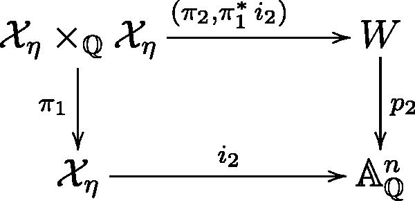
Here π1 and π2 are the first and second coordinate projections The map
from the bottom left to the top right, using the universal property of the product, gives rise to the diagonal section
of π1. Then, there is the identification
identifying the functions gi in
with the functions
in
In other words, if you express the gi in terms of the variables xj on
then you get
by replacing all the xj’s by zj’s.
The map is constructed in an analogous way to the construction of the map
It sends
to
where
on
Now the isomorphism
is constructed cf. [CitationLiu 02, Lem. 6.4.1, pp.. 236–237]. Of course,
Recall that where
is the embedding, and
is the sheaf of ideals on
defining
After base change to
this becomes
The result now follows immediately. □
Altogether, this leads to the following algorithm.
Algorithm 13.
Input: monic polynomial of degree
describing a hyperelliptic curve C of genus g over
Output: the real period Ω of its Jacobian J.
Step 1: calculate the so-called big period matrix of J, where the notation is as before, using the Magma command BigPeriodMatrix (due to Van Wamelen).
Step 2: for each subset with
calculate the covolume
Step 3: use Euclid’s algorithm to find a generator P for the lattice spanned by the PI.
Step 4: for each bad prime p, calculate a regular model of C, using the Magma command RegularModel. This will give us a representation of
by charts which are relative complete intersections.
Step 5: for each of the differentials check if it has a pole on any of the irreducible components of the special fiber of
If so, adjust the basis by multiplying the differential having a pole with p to get a new basis
and apply Step 5 again (until the basis is not changing anymore).
Step 6: for each check if
vanishes on the whole special fiber of
If so, adjust the basis
by replacing one of the ωj such that
with
then apply Step 6 again (until the basis is not changing anymore).
Step 7: for each bad prime p compute where a is the number of basis adjustments done in Step 5, and b is the number of basis adjustments done in Step 6 (this is also the determinant of the change of basis matrix whose columns express
in terms of
). Then take the product W over p of these determinants, and output
End.
4. Computation of other terms in BSD formula
Throughout this section, we will use the following notation.
Notation 14. We define to be a hyperelliptic curve of genus g. When a prime p is introduced,
is a regular model of H over
The Jacobian of H is denoted by J, and the Néron model of J over
is called
Moreover, we will assume that H is given by a model of the form where the input polynomial f(x) has odd degree. The reason we assume f(x) to have odd degree, is twofold. On the one hand, the existence of a rational Weierstraß point ensures the conditions of Theorem 7 are met. On the other hand, the Jacobian arithmetic has not been fully implemented in Magma for hyperelliptic curves without rational Weierstraß point.
4.1. Torsion subgroup and rank
In order to compute the torsion group and algebraic rank of J, we will be computing upper and lower bounds.
For the torsion, upper bounds are given by considering the reduction of J at good primes. For the algebraic rank, upper bounds are given by considering 2-Selmer groups. This is already implemented in Magma by Stoll.
To get lower bounds, we try to find as many points as possible on J. For genus 2, this is already implemented in Magma. For genus 3, 4, and 5, the author implemented a simple search algorithm for points, using the Mumford representation that Magma is using to represent points on J.
In fact, for Jacobians of curves J and are isomorphic. Hence, in order to verify the BSD conjecture up to squares in this case, it is actually not necessary to know the size of the torsion subgroup at all.
4.2. L-function
In this section, we will briefly discuss the computation of the special value of the L-function associated to the Jacobian of a hyperelliptic curve. For a complete definition and theoretical background on the L-function, see [CitationSerre 70].
The idea used to compute the L-function is as follows. The local L-factors at the good primes p > 2 can be found by counting points in for sufficiently many
In order to find the local L-factors at the bad places, one uses the functional equation. The idea is to guess, in a clever way, the conductor and, for the bad primes, the local L-factors, in such a way that the L-function obtained satisfies the conjectural functional equation, see also [CitationBooker et al. 16, sect. 5, pp. 243–245].
Remark 15.
To guess the 2-part of the conductor, the following naive version of Ogg’s formula is used:
Here, is the valuation of the (naive) minimal discriminant, n is the number of geometrically irreducible components in a minimal regular model, and
is our guess for the 2-valuation of the conductor. The formula, in this shape, does not give the correct 2-valuation of the conductor in general. For curves of genus 2 over a Henselian discrete valuation ring with algebraically closed residue field, we can deduce the formula
from [CitationLiu 94], where c(X), as defined in loc. cit., is a non-negative integer. Over general discrete valuation rings, the discriminant could change after a quadratic field extension, cf. [CitationLiu 96, Prop. 4, p. 4595]. In this case, it drops by
So, for genus 2, in case
the discriminant will apparently not change anymore, and c(X) = 0 must hold for the 2-valuation f of the conductor to not become negative. Hence, the naive version of Ogg’s formula holds in this case.
In [CitationDokchitser 04], Tim Dokchitser describes a trick with an inverse Mellin transform in order to actually evaluate the L-function. This has been implemented by him, together with Vladimir Dokchitser, in Magma. This is the method we used for our calculations. However, it is useful to remark that the runtime increases quickly when the conductor increases and that this could probably by remedied by using the methods from [Harvey et al. Citation16].
4.3. Regulator
Using the points on J that we found when computing the algebraic rank, we will compute the regulator. In order to do that, we need to calculate the height pairing for several pairs of points.
Due to work of Holmes [CitationHolmes 12] and Müller [CitationMüller 14] it is now known how arithmetic intersection theory could be used to do this calculation. This has also been implemented in Magma for Jacobians of hyperelliptic curves by Müller, and works in practice for genus up to 10.
In many cases, especially in genus 3, 4, and 5, the height bound we use for point finding is not high enough to provably compute the regulator. The upper bounds for difference between the naive and canonical height are quite big in some cases, see for example [CitationMüller and Stoll 16] for genus 2. In that case, we can only obtain a finite index subgroup of the Mordell-Weil group. Therefore, the regulator that we get might be a square multiple of the actual regulator of J. Hence, the conjectural order of assuming BSD, might be a multiple of the order that we compute.
4.4. Tamagawa numbers
Suppose that we have a regular model of H over the strict henselization of
Then in [CitationBosch and Liu 99, Thm. 1.1, p. 277], Bosch and Liu give an exact sequence
of
-modules. Here
is the geometric component group of the Néron model of
The map
with
indexing the components
of the special fiber of
maps each component Γj to
where
is the intersection pairing and ei is the geometric multiplicity of Γi (in itself, which is 1 in our case). The map
maps each component Γj to
where dj is the multiplicity of Γj in the special fiber. Here, the Galois group
acts on
by its natural action on the components of the special fiber.
Due to Donnely, Magma is able to compute this geometric component group using this theorem, and moreover, because explicit equations exist for a regular model of H over
we are able to compute the action of Frobenius on
and
The way regular models are constructed in Magma is by repeatedly blowing up non-regular points until the fibered surface is regular. To compute the Galois action on the components of the special fiber, we traced down this blow-up procedure, and in each step we computed the action of Galois on the points blown-up, and on the new components which appeared in the special fiber on the new blown-up charts.
The result is an implementation of a Magma package on top of the existing regular models package, which computes the action of the Galois group on and then computes the Tamagawa number, the order of
The source code for this package will be released together with this article. It has been used to compute Tamagawa numbers for the Jacobians associated to almost all of the 66,158 genus 2 curves present in [CitationLMFDB 00] (see also [CitationBooker et al. 16]). This computation was finished within a few hours.
4.5. Tate-Shafarevich group
For our calculations, we do not calculate the order of the Tate-Shafarevich group. Instead, we only check whether the conjectural order, given by the BSD conjecture, is (up to a certain precision) a rational square or two times a rational square (with a small denominator) according to the criteria described in [CitationPoonen and Stoll 99].
Acknowledgements
The author wishes to thank his supervisors David Holmes and Fabien Pazuki. Moreover, Tim Dokchitser and Steffen Müller are thanked for their advise and insight, Carlo Pagano is thanked for helping with the proof of a lemma, and anonymous referees are thanked for the comments they provided to improve this article.
Related Research Data
References
- [Booker et al. 16] A. R. Booker, J. Sijsling, A. Sutherland, J. Voight, D. Yasaki. “A database of genus-2 curves over the rational numbers.” LMS J. Comput. Math. 19:suppl. A (2016), 235–254.
- [Birch and Swinnerton-Dyer 65] B. J. Birch, H. P. F. Swinnerton-Dyer. “Notes on elliptic curves. II.” J. Reine Angew. Math. 218 (1965), 79–108.
- [Bosch and Liu 99] S. Bosch, Q. Liu. “Rational points of the group of components of a Néron model.” Manuscr. Math. 98:3 (1999), 275–293.
- [Bosch et al. 90] S. Bosch, W. Lütkebohmert, M. Raynaud, Néron models. Berlin: Springer, 1990.
- [Dokchitser 04] T. Dokchitser, “Computing special values of motivic L-functions.” Exp. Math. 13:2 (2004), 137–149.
- [Flynn et al. 01] E. V. Flynn, F. Leprévost, E. F. Schaefer, W. A. Stein, M. Stoll, J. Wetherell, “Empirical evidence for the Birch and Swinnerton-Dyer conjectures for modular Jacobians of genus 2 curves.” Math. Comp. 70:236 (2001), 1675–1697.
- [Harrison 18] M. Harrison, Small hyperelliptic curves over Q. Retrieved on 26 June 2018 from https://people.maths.bris.ac.uk/∼matyd/HE/.
- [Harvey et al. 16] D. Harvey, M. Massierer, A. S. Sutherland, “Computing L-series of geometrically hyperelliptic curves of genus three.” LMS J. Comput. Math. 19:suppl. A (2016), 220–234.
- [Hindry and Silverman 2000] M. Hindry, J. H. Silverman. Diophantine geometry. An introduction. New York: Springer, 2000.
- [Holmes 12] D. Holmes, “Computing Néron-Tate heights of points on hyperelliptic Jacobians.” J. Number Theory 132:6 (2012), 1295–1305.
- [Kolyvagin 89] V. A. Kolyvagin, “Finiteness of E(Q) and Ш(E,Q) for a subclass of Weil curves.” Math. USSR-Izv. 32:3 (1989), 523–541.
- [Kolyvagin 91] V. A. Kolyvagin, On the Mordell-Weil group and the Shafarevich-Tate group of modular elliptic curves. International Congress of Mathematicians, vol. I, II (Kyoto, 1990), 429–436. Math. Soc. Japan, Tokyo, 1991.
- [Liu 94] Q. Liu, “Conducteur et discriminant minimal de courbes de genre 2.” Compos. Math. 94:1 (1994), 51–79.
- [Liu 96] Q. Liu, “Modèles entiers des courbes hyperelliptiques sur un corps de valuation discrète.” Trans. Amer. Math. Soc. 348:11 (1996), 4577–4610.
- [Liu 02] Q. Liu, Algebraic geometry and arithmetic curves. Oxford: Oxford University Press, 2002. Translated by R. Erné.
- [LMFDB] The LMFDB Collaboration, The L-functions and Modular Forms Database. Available at: http://www.lmfdb.org.
- [Milne 72] J. S. Milne, “On the arithmetic of abelian varieties.” Invent. Math. 17 (1972), 177–190.
- [Milne 86] J. S. Milne, “Jacobian varieties.” In Arithmetic geometry (Storrs, Conn., 1984), pp. 167–212. Springer, New York, 1986.
- [Müller 14] J. S. Müller, “Computing canonical heights using arithmetic intersection theory.” Math. Comp. 83:285 (2014), 311–336.
- [Müller and Stoll 16] J. S. Müller, M. Stoll, “Canonical heights on genus-2 Jacobians.” Algebra Number Theory 10:10 (2016), 2153–2234.
- [Poonen and Stoll 99] B. Poonen, M. Stoll, “The Cassels-Tate pairing on polarized abelian varieties.” Ann. Math. 150:3 (1999), 1109–1149.
- [Raynaud 70] M. Raynaud, “Spécialisation du foncteur de Picard.” Inst. Hautes Études Sci. Publ. Math. 38 (1970), 27–76.
- [Serre 70] J. P. Serre, “Facteurs locaux des fonctions zêta des variétés algébriques (définitions et conjectures).” Séminaire Delange-Pisot Poitou. Théorie des nombres, 11 (1969–1970), no. 2, Talk no. 19, pp. 1–15.
- [Tate 66] J. Tate, “On the conjectures of Birch and Swinnerton-Dyer and a geometric analog.” Séminaire Bourbaki, 9 (1964–1966), Exp. No. 306, pp. 415–440