
 ?Mathematical formulae have been encoded as MathML and are displayed in this HTML version using MathJax in order to improve their display. Uncheck the box to turn MathJax off. This feature requires Javascript. Click on a formula to zoom.
Abstract
In this paper, we propose combining the stochastic blockmodel and the smooth graphon model, two of the most prominent modeling approaches in statistical network analysis. Stochastic blockmodels are generally used for clustering networks into groups of actors with homogeneous connectivity behavior. Smooth graphon models, on the other hand, assume that all nodes can be arranged on a one-dimensional scale such that closeness implies a similar behavior in connectivity. Both frameworks belong to the class of node-specific latent variable models, entailing a natural relationship. While these two modeling concepts have developed independently, this paper proposes their generalization towards stochastic block smooth graphon models. This combined approach enables to exploit the advantages of both worlds. Employing concepts of the EM-type algorithm allows to develop an appropriate estimation routine, where MCMC techniques are used to accomplish the E-step. Simulations and real-world applications support the practicability of our novel method and demonstrate its advantages. The paper is accompanied by supplementary material covering details about computation and implementation.
Disclaimer
As a service to authors and researchers we are providing this version of an accepted manuscript (AM). Copyediting, typesetting, and review of the resulting proofs will be undertaken on this manuscript before final publication of the Version of Record (VoR). During production and pre-press, errors may be discovered which could affect the content, and all legal disclaimers that apply to the journal relate to these versions also.1 Introduction
The statistical modeling of complex networks has gained increasing interest over the last two decades, and much development has taken place in this area. Network-structured data arise in many application fields and corresponding modeling frameworks are used in sociology, biology, neuroscience, computer science, and others. To demonstrate the state of the art in statistical network data analysis, survey articles have been published by Goldenberg et al. (2009), Snijders (2011), Hunter et al. (2012), Fienberg (2012), and Salter-Townshend et al. (2012). Furthermore, comprehensive monographs in this field are given by Kolaczyk (2009), Lusher et al. (2013), Kolaczyk and Csardi (2014), and Kolaczyk (2017).
In order to capture the underlying structure within a given network, various modeling strategies based on different concepts have been developed. One ubiquitous model class in this context is given by the Node-Specific Latent Variable Models, see Matias and Robin (2014) for an overview. This rather broad framework follows the assumption that the edge variables Yij
, of a network consisting of the node set
can be characterized as independent when conditioning on the node-specific latent quantities
. To be precise, the generic model design can be formulated via independent Bernoulli random variables with corresponding success probabilities, i.e.
(1)
(1) where
characterizes an overall connectivity pattern. This especially means that the connection probability for node pair (i, j) depends exclusively on the associated quantities
and
. Depending on the concrete model specification, these quantities are either random variables themselves or simply unknown but fixed parameters. Moreover,
can be multivariate, even though it is used as a scalar in many frameworks. Lastly, data-generating process (1) is generally defined for any
. However, in the case of undirected networks without self-loops, it is only performed for i < j, with the additional settings of
and
. This scenario is what we focus on in this work.
The general framework sketched above includes several well-known models in the field of statistical network analysis. The most popular ones of this type are the Stochastic Blockmodel (Holland et al., 1983, Snijders and Nowicki, 1997 and 2001) as well as its variants (Airoldi et al., 2008, Karrer and Newman, 2011), the Latent Distance Model (Hoff and coauthors, 2002, 2007, 2009, 2021, Ma et al., 2020), and the Graphon Model (Lovász and coauthors, 2006, 2007, 2010, Diaconis and Janson, 2007). Sharing the notion of a connectivity structure that depends only on node-specific latent variables apparently implies a natural relationship between these modeling approaches. At the same time, it is well known that they possess very different capacities for representing the diverse structural aspects discovered in real-world networks. In the context of concrete data analysis, it is often unknown beforehand what the requirements in terms of structural expressiveness are. Consequently, choosing the modeling strategy which is most suitable to capture the present network structure is a difficult task in itself. To detect the best method from an ensemble of models and corresponding estimation algorithms, Li et al. (2020) recently developed a cross-validation procedure for model selection in the network context, see also Gao and Ma (2020). One step further, Ghasemian et al. (2020) and Li and Le (2023) discuss mixing several model fits based on different weighting strategies.
Although all node-specific latent variable models are more or less closely related by construction, little attention has been paid to the proper representation or integration of one model by another or to combining multiple models in a joint framework. As an advantage, such a model unification provides a new perspective and potentially a more flexible modeling strategy. Steps in this direction have been taken by, for example, Fosdick et al. (2019, Sec. 3), who developed a Latent Space Stochastic Blockmodel by modeling the within-community structure as a latent distance model. Similarly, Schweinberger and Handcock (2015) combined the stochastic blockmodel with the Exponential Random Graph Model (ERGM). ERGMs are, however, beyond formulation (1) and instead seek to model the frequencies of prespecified structural patterns through a direct parameterization.
In this paper, we pick up the idea of model (1) but aim to formalize and estimate the underlying connectivity structure in a way that allows us to unite previous approaches. To do so, we combine stochastic blockmodels with (smooth) graphon models, leading to an extension that is able to capture the expressiveness of both models simultaneously. In order to fit this model to network data, we utilize previous results on smooth graphon estimation (Sischka and Kauermann, 2022) and EM-based stochastic blockmodel estimation (Daudin et al., 2008, De Nicola et al., 2022). The resulting method is flexible and feasible for networks with several hundred nodes.
The rest of the paper is structured as follows. In Section 2, we begin with a brief description of stochastic blockmodels and smooth graphon models, based on which we subsequently derive our generalized modeling approach. For the estimation, we develop an EM-type algorithm, which is elaborated in Section 3. This includes the formulation of a criterion for choosing the number of groups. The capability of our method is demonstrated in Section 4, which is done with respect to simulations and real-world networks. The discussion in Section 5 completes the paper.
2 Stochastic Block Smooth Graphon Model
2.1 Stochastic Blockmodel
In the literature on statistical network analysis, the stochastic blockmodel (SBM) is an extensively developed tool for modeling group structures in networks, see Newman (2006), Choi et al. (2012), Peixoto (2012), Bickel et al. (2013), and others. In its classical version, one assumes that each node, , can be uniquely assigned to one of
groups such that the probability of two nodes being connected only depends on their group memberships. Reversely, the data-generating process can be formulated as two successive steps. First, we draw the node assignments Zi
,
independently from a categorical distribution given through
(2)
(2)
Based on that, the edge variables are simulated under conditional independence through(3)
(3) for i < j, where
and
by definition. In these formulations,
represents the vector of (expected) group proportions and
is the corresponding entry of the block-related edge probability matrix
. Referring to formulation (1), this construction is apparently equivalent to setting
and
. Moreover, this modeling framework can also be viewed as a mixture of Erdős-Rényi-Gilbert models (Daudin et al., 2008). This is because the edge variables between all pairs of nodes from two particular groups or within one group are assumed to be independent and to have the same probability. Since very often, the connectivity within groups is relatively intensive, groups are also referred to as communities.
Although the model formulation is simple, the estimation is not straightforward. This is because both the latent community memberships and the model parameters need to be inferred from the data. The literature of a posterior blockmodeling starts with the works of Snijders and Nowicki (1997, 2001) and since then has been elaborated extensively (Handcock et al., 2007, Decelle et al., 2011, Rohe et al., 2011, Choi et al., 2012, Peixoto, 2017). As an additional hurdle in this framework, also the number of communities has usually to be estimated. Works taking this issue into account or specifically focusing thereon are, among others, Kemp et al. (2006), Wang and Bickel (2017), Chen and Lei (2018), Newman and Reinert (2016), Riolo et al. (2017), and Geng et al. (2019).
2.2 Smooth Graphon Model
Another modeling approach that utilizes latent quantities to capture complex network structure is the graphon model. As a fundamental difference to the discretely parameterized SBM , the graphon model formalizes a continuous specification, where the induced data-generating process can again be formulated via two successive steps. First, the latent quantities are independently drawn from a uniform distribution, i.e.
(4)
(4)
for . Then, the network entries are sampled conditionally independently in the form of
(5)
(5) for i < j, where again
and
. The bivariate function
is the so-called graphon. Choosing
and
yields the representation in the form of (1). In comparison with the SBM, the graphon model facilitates more flexible structures. This is because the possibilities for the manifestation of
are virtually unlimited, implying a higher potential complexity than for
, especially for small K, which is the more common setting. At the same time, it is possible to construct the graphon model such that it covers any stochastic blockmodel, see e.g. Latouche and Robin (2016, Fig. 1) or De Nocola et al. (2022, Sec. 3.3). However, when it comes to estimation, the enormous complexity of
is problematic and thus must be brought under control by applying additional constraints. A common approach to do so is to assume smoothness, meaning that
fulfills some Hölder or Lipschitz condition (Olhede and Wolfe, 2014, Gao et al., 2015, Klopp et al., 2017). This framework is what we call Smooth Graphon Model (SGM). Relying on this smoothness assumption, many works apply histogram estimators, often also interpreted as SBM-type approximations, see e.g. Wolfe and Olhede (2013), Airoldi et al. (2013), Chan and Airoldi (2014), or Yang et al. (2014). In order to get a continuous function out of such a piecewise constant representation, Li et al. (2022) specify graphons by constructing the value at each position
through a mixture over such blockwise probabilities, defining the weights as continuous functions of (u, v). As another approach to continuous graphon estimation, Lloyd et al. (2012) formulate a Bayesian modeling framework with Gaussian process priors, see also Orbanz and Roy (2015) for a more general formulation. Sischka and Kauermann (2022) guarantee a smooth and stable estimation of
by making use of (linear) B-spline regression. In contrast to the previous strategies, some works waive strict smoothness assumptions on
, see Chatterjee (2015) and Zhang et al. (2017). Note, however, that these methods are not intended to estimate
but solely the edge probabilities
.
2.3 Stochastic Block Smooth Graphon Model
Both the SBM and SGM are based on underlying assumptions which appear to be needlessly restrictive conditions—namely strict homogeneity within the communities and overall smoothness, respectively. As an alternative, we pursue to design a new model class which does not suffer from such limitations. To do so, we combine the two modeling approaches towards what we call a Stochastic Block Smooth Graphon Model (SBSGM). To be specific, we assume the node assignments Zi
to be drawn from (2) and draw independently Ui
from (4) for . Then (3) and (5) are replaced by
(6)
(6) where, for each pair of groups and also within groups, connectivity is now formulated by an individual smooth graphon
with
. Apparently, if K = 1 we obtain an SGM, while all
being constant yields an SBM.
This model can be reformulated in a compact form by conflating the node assignments (2) and the latent quantities (4) and compressing the model specification onto a single square. To be precise, we draw Ui
from (4) and, given Ui
, , we sample
(7)
(7) for i < j, where
is a partitioned graphon which is smooth within the blocks spanned by
, meaning within
for
. More precisely, transforming the formulation from (6) to (7) implies that
and
with
being given through
, i.e.
. We also here remain with the common convention of symmetry (
) and the absence of self-loops (
). An exemplary SBSGM together with a simulated network is illustrated in Figure 1. As a special property in terms of expressiveness, this model allows for smooth local structures under a global division into groups.
The assumption of a graphon that is not overall but only piecewise smooth has already been applied before, see e.g. Airoldi et al. (2013) or Zhang et al. (2017). Nonetheless, there is a major conceptional distinction in the modeling perspective pursued here. While in previous works, lines of discontinuity were merely allowed, we now explicitly incorporate them in the modeling context as structural breaks. This novel modeling approach—which also rules the estimation—has a substantial impact on uncovering the network’s underlying structure. The fact that previous graphon estimation approaches are not able to fully capture block structures is showcased, for example, by Li and Le (2023), who observe an improvement in accuracy when mixing graphon fits with SBM estimates. In Section 4, we demonstrate that our method enables capturing both block structures and smooth within-group differences, for which we rely on synthetic and real-world networks.
2.4 Piecewise Smoothness and Semiparametric Formulations
In general, we define the SBSGM to be specified by a piecewise Lipschitz graphon with horizontal and vertical lines of discontinuity. More precisely, for , that means that there exist boundaries
and a constant
such that for all
(8)
(8) for any
, where
is the Euclidean norm. We indicate this attribute in the notation by making use of the subscript
, meaning that
is piecewise Lipschitz continuous with respect to
. In the case of M = 0, this implies the representation of an SBM, whereas
indicates an SGM.
To achieve a semiparametric framework from this theoretical model formulation, we follow the spline-based approach of Sischka and Kauermann (2022), extending it to the piecewise smooth format. This can be realized by constructing a mixture of B-splines. To be precise, we formulate blockwise B-spline functions on disjoint bases in the form of(9)
(9) where ⊗ is the Kronecker product and
is a linear B-spline basis on
, normalized to have maximum value 1 (see Figure 2 for a color-coded exemplification). The inner knots of the k-th one-dimensional B-spline component with length Lk
are denoted by
, where
and
. Moreover,
denotes the overall vector of B-spline knots, and the complete parameter vector is given in the form of
with
.
This piecewise B-spline representation serves as suitable approximation of , where the approximation error
can be arbitrarily reduced by increasing
accordingly. In general, we choose a sufficiently large total basis length
, which is then divided among the segments in proportion to their extents. The Lk
inner knots of the k-th component are subsequently located equidistantly within
, which completes the specification of B-spline formulation (9).
The above representation allows to apply penalized B-spline regression readily. The capability of such a framework as well as the general role of penalized semiparametric modeling concepts are discussed, for example, by Eilers and Marx (1996), Ruppert et al. (2003), Wood (2017), and Kauermann and Opsomer (2011).
3 EM-Type Algorithm
For fitting the SBSGM to a given network, the latent positions and the parameters
and
need to be estimated simultaneously. This is a typical task for an EM algorithm, which aims at deriving information about unknown quantities in an iterative manner. In this regard, it is important to stress that SBSGMs suffer from non-identifiability in the same way as graphon models. In fact, an SBSGM is defined only up to an equivalence class. See our Supplementary Material for more details. Generally and simply speaking, the assumption of smoothness within communities works towards identifiability. The number of structural breaks, on the other hand, is assumed to be given for now. A discussion on how to infer K from data is given in Section 3.3.
3.1 MCMC E-Step
The conditional distribution of U given y is rather complex, and hence calculating the expectation cannot be solved analytically. Therefore, we apply MCMC techniques for carrying out the E-step. In that regard, the full-conditional distribution of Ui
can be formulated as(10)
(10)
Based on that, we can construct a Gibbs sampler, which allows consecutive drawings for . For its concrete implementation, we replace
by its current estimate. Finally, we derive reliable means for the node positions by appropriately summarizing the MCMC sequence. Technical details are provided in the Appendix.
In this scenario, however, we are faced with an additional identifiability issue, which we want to motivate as follows. Assume first an SBSGM as in (7), but allow the distribution of the latent quantities Ui
to be not necessarily uniform but arbitrarily continuous instead. Under this condition, the SBSGM specification is broadened to with
as the distribution of the Ui
’s. An equivalent network-generating process can then not only be constructed through permutations (formulation (4) of the Supplementary Material) but also by taking any strictly increasing continuous transformation
and specifying
and
(11)
(11) with
for
. Note that in these formulations,
implies a modification of the probability measure on the domain
, and therefore it is no measure-preserving transformation—except for
. The two models
and
are then not distinguishable in terms of the probability mass function induced on networks, causing an additional identifiability issue which, in fact, cannot be resolved by the EM algorithm. As a matter of conception, the EM algorithm aims at determining a model specification that optimally fits the data and not at accurately recovering the underlying model framework. Consequently, this issue needs to be handled post hoc, where we aim for model specification
with
representing the uniform distribution. We tackle this issue by making use of two separate transformations
, adjusting between and within groups, respectively. This is sketched in Figure 3, where we demonstrate both the theoretical and the empirical implementation. Adjustment 1 ensures that the extent of a component complies with its associated probability mass or relative frequency, respectively. This also involves adapting the component boundaries, which is analogous to adjusting community proportions in the blockmodeling framework. Adjustment 2 effects that the distribution within groups is uniform. Further details on the concrete implementation in the algorithm are given in the Appendix. We denote the final result of the E-step in the m-th iteration, i.e. the outcome achieved through Gibbs sampling and applying Adjustment 1 and Adjustment 2, by
.
3.2 M-Step
3.2.1 Linear B-Spline Smoothing
In consequence of representing the SBSGM as a mixture of (linear) B-splines as in (9), we are now able to view the estimation as semiparametric regression problem, which can be solved via maximum likelihood approach. Given the spline formulation, the full log-likelihood results inwhere
and
is the B-spline basis on
. Taking derivatives leads to score function and Fisher matrix, explicitly given in the Supplementary Material. Based on that,
can be maximized using Fisher scoring. To guarantee that the resulting estimate of
fulfills symmetry and boundedness, we additionally impose (linear) side constraints on
. First, to accommodate symmetry, we require that
for all
and
. Second, the condition of
being bounded to
can be formulated as
. These two side constraints are of linear form and can be incorporated through
and
with matrices G and A chosen accordingly. Here,
and
are vectors of corresponding sizes. Consequently, maximizing
with respect to the postulated side constraints can be considered as an (iterated) quadratic programming problem, which can be solved using standard software (see e.g. Andersen et al., 2016 or Turlach and Weingessel, 2013).
3.2.2 Penalized Estimation
Following the ideas underlying the penalized spline estimation (see Eilers and Marx, 1996 or Ruppert et al., 2009), we additionally impose a penalty on the coefficients to achieve smoothness. This is necessary since we intend to choose the total basis length L of the mixture of B-splines to be large and unpenalized estimation will lead to wiggled estimates. For inducing smoothness within the components, we penalize the difference between “neighboring” elements of . Let therefore
be the first-order difference matrix. We then penalize
and
, where
is the identity matrix of size Lk
. This leads to the penalized log-likelihood
where
is the diagonal matrix
with
and
serving as vector of smoothing parameters for the respective blocks. In this configuration, the resulting estimate apparently depends on the penalty parameter vector
. Setting
for
yields an unpenalized fit, while setting
leads to a piecewise constant SBSGM, i.e. an SBM. Therefore, the smoothing parameter vector
needs to be chosen in a data-driven way. For example, this can be realized by relying on the Akaike Information Criterion (AIC) (see Hurvich and Tsai, 1989 or Burnham and Anderson, 2002). This is a common framework for penalized estimation and in the interest of space we provide details in the Supplementary Material. Following this overall procedure finally leads us to parameter estimate
in the
-th iteration of the EM algorithm.
3.3 Choice of the Number of Communities and Numerical Complexity
As for the SBM, the number of communities, K, is an essential parameter that, in real-world networks, is usually unknown. Preferably, this should also be inferred from the data. For this purpose, we take up two different intuitions, which can finally be brought together to construct an appropriate model selection criterion.
On the one hand, one might think of adopting methods for determining the number of communities from the SBM context. A common strategy under this framework relies on the Integrated Classification Likelihood ( ) criterion (Daudin et al., 2008, Côme and Latouche, 2015, Mariadassou et al., 2010). However, for applying this to the SBSGM, one needs to observe the more complex structure. This is especially so because the structural complexity within communities and the number of groups can compensate for each other to a certain extent.
As an alternative approach, one could exploit the AIC elaborated for choosing by extending it towards a model selection strategy with respect to K. This can be accomplished by adding a corresponding term, for which we propose to apply the concept of the Bayesian Information Criterion (BIC). Combined with the previous formulation, this yields a mixing of AIC and BIC. To be precise, we select the smoothing parameter using the AIC as described above, but for the number of blocks, we impose a stronger penalty by replacing the factor of two with the logarithmized sample size. We consider this to be in line with Burnham and Anderson (2004), who conclude that the AIC is more reliable when the ground truth can be described through many tapering effects (smooth within-community structure), whereas the BIC is preferable when there exist only a few large effects (number of blocks). The criterion obtained according to this conception then is, in fact, equivalent to the ICL up to a different parameterization of the log-likelihood and an additional term for penalizing the smooth structure within communities. When setting
for
, the criterion even reduces exactly to the ICL for SBMs. Details on the construction as well as the concrete specification are given in the Supplementary Material.
Note that, taken together, the presented estimation routine might appear to be time-consuming and computationally intensive when compared to more efficient algorithms for related models. However, we emphasize that such approaches cannot be simply adopted due to the higher complexity of the SBSGM. In this regard, utilizing MCMC techniques in the E-step of an EM algorithm is a well-known concept for fitting complex models with latent variables, see e.g. Wei and Tanner (1990, Remark 1), McCulloch (1994, Sec. 4.2), and Levine and Casella (2001). A reduction of the computational costs for the Gibbs sampler can, in this setting, be achieved by using as reliable starting values in the E-step of the m-th iteration, making the need of multiple burn-in phases obsolete. Moreover, as suggested by Wei and Tanner (1990, Sec. 3.1) and McCulloch (1994, Sec. 4.2), the sample size of the MCMC sequence can be chosen rather small in the beginning, which then will only be increased in later iterations of the EM algorithm.
Such an iterative procedure not only enables a general estimation but also promises high accuracy, as demonstrated by the application studies in Section 4. A detailed discussion on the computational intensiveness is given in the Supplementary Material. We will show in the application section below, that alternative approaches—though numerically faster—lead to weaker performance measures.
4 Application
We investigate the performance of our approach with respect to both simulated and real-world networks. For an “uninformed” implementation, we initialize the algorithm by setting to a random permutation of
. At the same time, we place the community boundaries equidistantly within
, i.e. we set
for
. Since different initializations might lead to different final results, we repeat the estimation procedure with varying random permutations for
and, in the end, choose the best outcome. In our experience, five to ten random repetitions already lead to quite satisfactory results in the sense that further repetitions do not provide substantial improvement. Moreover, if the number of groups is unknown beforehand, we fit the SBSGM with varying K and employ the criterion from Section 3.3 to select the optimal estimate. The variability in the estimation result for different initializations of U and choices of K is illustrated for all of the following applications in Figure 9 of the Supplementary Material.
4.1 Synthetic Networks
In the scenario of simulations, we order the final estimate according to the representation format of the ground-truth model, which involves the within- and between-group arrangement. That is, we permute the final estimate of in terms of swapping communities and reversing within-group arrangements from back to front if visibly adequate.
4.1.1 Assortative Group Structure with Smooth Differences
To showcase the general applicability of our method, we first consider again the SBSGM from Figure 1 together with the associated simulated network of size N = 500. Starting with determining the number of groups, the first row of Table 1 shows the corresponding values of the criterion for choosing K. This suggests the correct number of three communities. The corresponding estimation result, meaning for K = 3, is illustrated in Figure 4, which clearly demonstrates that the estimate of (top right plot) precisely captures the structure of the true model (top left). In line with this, the comparison of estimated and simulated node positions (bottom right) reveals that the latent quantities are appropriately recovered. To be precise, according to the relation between
and
, the groups are accurately assigned, and, in addition, also the within-community positions are well replicated. Altogether, the underlying structure can be precisely uncovered.
4.1.2 Core-Periphery Structure
As a second simulation example, we consider model (a) of Figure 5, where an equivalent representation is also given by model (a2). Apparently, the “true” number of groups here is K = 1, meaning that arrangement (a) is preferred. Hence, this is the structure that should be adopted by the estimation procedure, regardless of the choice of K. We demonstrate that our algorithm adheres to this by fitting the model with both settings, K = 1 and K = 2. This gives additionally a better intuition of the algorithm’s proceeding. The estimation results for simulated networks of size N = 500 are illustrated by ( ) and (
), respectively. Obviously, both estimates follow the “single-community” representation, which exemplifies the method’s general implicit strategy of merging similarly behaving nodes. In addition, a comparison of the estimates with regard to minimizing the group-number criterion (see second row of Table 1) reveals that the model fit with K = 1 appears preferable over the one with K = 2.
4.1.3 Mixture of Assortative and Disassortative Structures under Equal Overall Attractiveness
Following on from the two-group representation (a2) of the model above, we now construct an altered version. Instead of nodes being generally either weakly or strongly connected, they should now be either strongly connected within their own group and weakly connected into the respective other group or vice versa. This leads us to SBSGM specification (b) of Figure 5. More precisely, all nodes in this model have the same expected degree, where nodes being weakly connected within their own community compensated for their lack of attractiveness by reaching out to members of the respective other community. This kind of structure clearly cannot be collapsed to a single-community SBSGM. More importantly, it also cannot be captured by a degree-corrected SBM, where nodes are assumed to possess a uniform attractiveness. Our algorithm is however still able to fully capture the underlying structure, as shown by estimate ( ). Note that applying the criterion for choosing K in this case actually suggests one group (third row of Table 1). This wrong specification might be caused by the fact that the structural break at 0.5 is only half (namely from 0 to 0.5). Besides, the decision is quite close compared to the setting of K = 2.
4.2 Real-World Networks
For evaluating our method with regard to real-world data, we consider three networks from different domains, comprising social and political sciences as well as neurosciences. These networks also vary in their inherent structure, including the overall density. An overview of the networks’ most relevant summarizing attributes is given in Table 2. For brevity, the complete analysis of the military alliance network can be found in the Supplementary Material.
4.2.1 Political Blogs
The political blog network has been assembled by Adamic and Glance (2005) and consists of 1222 nodes (after extracting the largest connected component). These nodes represent political blogs of which 586 are liberal and 636 are conservative, according to manual labeling (Adamic and Glance, 2005). An edge between two blogs illustrates a web link pointing from one blog to another within a single-day snapshot in 2005. For our purpose, these links are interpreted in an undirected fashion. The resultant network is illustrated in the top plot of Figure 6, with nodes exhibiting political labels. Note that this is the same network used by Karrer and Newman (2011) for demonstrating the enhancement achieved through their degree-corrected variant of the SBM. The criterion for K here suggests an SBSGM with K = 2 (see fourth row of Table 1), which is in accordance with the number of political orientations. Moreover, the model-based node assignment is very close to the manual labeling, as indicated by the network representation at the bottom right (see also Figure 5 of the Supplementary Material). Information beyond community membership prediction can be gained by analyzing the relative node positions within groups. This internal ordering reveals, for example, a within-group structure that is dominated by a division into core and periphery nodes, which is also indicated by the locally bounded intense regions in the estimate of (bottom left plot). The emergence of such a core-periphery structure is a well-known phenomenon in the linking of the World Wide Web, of which the considered blogs are an extraction. In a more specific sense, this core-periphery structure mirrors the blogs’ “sociability,” i.e. their involvement in the political discourse. A further structural aspect revealed by the model fit is the domination of an assortative structure, signalized by an overall intensity that is much higher within than between the two communities. Together with the inferred grouping by political orientations, this indicates that blogs tend to link to blogs from the same political side rather than to blogs of the respective other side.
4.2.2 Human Brain Functional Coactivations
As a second real-world data example, we consider the human brain functional coactivation network. This network has been assembled by Crossley et al. (2013) via meta-analysis and is accessible through the Brain Connectivity Toolbox (Rubinov and Sporns, 2010). More precisely, the provided weighted network matrix represents the “estimated […] similarity (Jaccard index) of the activation patterns across experimental tasks between each pair of 638 brain regions” (Crossley et al., 2013), where this similarity is additionally “probabilistically thresholded.” Based on that, we construct an unweighted graph by including a link between all pairs of brain regions which have a significant similarity, meaning a positive score in the original data set. For the arising network, determining the number of groups based on the proposed criterion yields three communities (see last-but-one row of Table 1). The decision, however, seems rather tight, and Crossley et al. (2013) choose a regular SBM with four communities for fitting these data. Hence, we also here choose K = 4, which allows a more direct comparison of the results (see Supplementary Material). The outcome of the SBSGM estimation under this setting is illustrated in Figure 7, where also here (top left) reveals an assortative structure. However, it is comparatively less pronounced, implicating that similar behavior and connectedness are less strongly associated. Furthermore, transferring the estimated node positions to the representation of brain regions in anatomical space exhibits a clearly visible arrangement. On the one hand, it seems that, according to functional coactivation, the complete realm of the brain can be divided into areas that are locally more or less solidly connected. On the other hand, relative positions within communities allow to infer a fragmentation beyond the strict clustering of nodes. For example, the community of reddish nodes further subdivides into a rear and a central front part, as recognizable in the side view representation. Overall, the visibly strong concordance between the network-related and the anatomical embedding of brain regions suggests that the underlying structure has been uncovered quite accurately. For the sake of completeness, the SBSGM fit with K = 3 is illustrated in the Supplementary Material. The results look quite similar, but they reveal a more extensive exploitation of capturing group structures through smooth differences. Moreover, for a last real-world analysis considering the military alliances among the world’s nations, we refer the reader to the Supplementary Material.
The results of all application studies together, it can be demonstrated that our novel approach is a very flexible modeling tool that yields a meaningful and interpretable outcome. In particular, the strict node clustering paired with relative positions within groups provides greater insights than previous approaches, making the SBSGM an outstanding tool for drawing more profound scientific conclusions. In addition, the SBSGM has been visually demonstrated to capture the structure within complex networks quite precisely. As a final step of this application study section, we aim for investigating the capacity of uncovering underlying network structures more quantitatively.
4.3 Performance in Prediction Accuracy
For a quantitative assessment of the method’s performance, we rely on prediction accuracy, which is differently specified for simulations and real-world scenarios. Moreover, to enable a proper evaluation of the performance results, we additionally apply the most prevalent methods for uncovering complex structure to the same networks. To be precise, as competing methods, we consider the degree-corrected stochastic blockmodel (DCSBM, Karrer and Newman, 2011), the universal singular value thresholding strategy (USVT, Chatterjee, 2015), and the neighborhood smoothing approach (NBSM, Zhang et al., 2017). For these modeling techniques, we employ the software packages graspologic (DCSBM, Jaewon et al., 2019) and randnet (USVT and NBSM, Li et al., 2021).
In the simulation setting, the prediction accuracy can be defined based on the differences between true and inferred edge probabilities. To be precise, we consider the root-mean-squared prediction error
The corresponding results for the model specifications from Section 4.1 and the associated simulated network data are illustrated in the top plot of Figure 8. For the scenario with smoothly varying assortative structures (Section 4.1.1/Figure 4), our method is slightly better than the competing approaches, where, altogether, the differences between the methods’ performances are rather small. For the core-periphery structured model from Section 4.1.2 (plot (a) of Figure 5), the DCSBM and the SBSGM perform distinctly better than the methods USVT and NBSM. The high accuracy of the DCSBM can be explained by the fact that the data-generating model can be exactly represented as single-community SBM with degree heterogeneity. In contrast, the specification from Section 4.1.3 (model (b) of Figure 5), which describes a mixture of assortative and disassortative structures, can noticeably be best modeled by the SBSGM. This is as expected since the structural assumptions of all the competing methods are only poorly met.
In the next step, we evaluate the performance on the real-world examples. To do so, we rely on the prediction accuracy with respect to randomly chosen network entries that have been replaced by “structureless” noise (for details, see Section 4 of the Supplementary Material). A proper quantification can then be constructed by relying on the Precision Recall (PR) relation, which follows the assumption of an unbalanced ratio between present and absent edges. For comparison reasons, we additional provide the results for the Receiver Operating Characteristic in the Supplementary Material. The Area-Under-the-Curve (AUC) metric additionally provides a scalar reference value. The corresponding results for the real-world networks from Section 4.2 are illustrated in the bottom row of Figure 8. For all three examples, the PR curve of the SBSGM exhibits a profile that is (almost) as good as or dominates the other ones, which is also underpinned by the corresponding AUC value. As further evidence of the SBSGM’s reliability, none of the three competing methods performs comparatively overall well, leading to an unclear ranking among them. The political blog and the human brain network reveal better performance results under USVT. This is not the case for the military alliance network, where the DCSBM and NBSM perform almost equally well but better than USVT. Altogether, the results obtained here coincide with the findings of Li and Le (2023), according to which a mixing of inferred block structures and graphon estimates leads to an improvement in prediction accuracy. Since our method is able to capture the different structural aspects of block structures and smooth differences simultaneously, the resulting performance results are somehow expected.
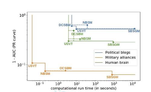
Finally, for a more thorough comparison, we plot prediction accuracy against run time. The results for all three real-world examples are illustrated in Figure 9, where, in addition, the resulting Pareto front is outlined. This demonstrates that the higher accuracy of the SBSGM comes at the cost of higher computation time. Still, if the focus is on accuracy and interpretability, our model appears to be often the better choice.
5 Discussion and Conclusion
Despite their close relationship, the stochastic blockmodel and the (smooth) graphon model have mainly been developed separately until now. To address this shortcoming, we proposed a combination of the two model formulations, leading us to a novel modeling approach that generalizes the two detached concepts in a unified framework. The resulting stochastic block smooth graphon model consequently unites the individual capabilities of the two initial approaches. These are the clustering of networks (SBM) and the capturing of smooth differences in the connectivity behavior (SGM). Utilizing previous results on SBM and SGM estimation allowed us to develop an EM-type algorithm for reliably estimating the (semiparametric) model specification.
Although the SBSGM arises from combining SBMs and SGMs, connections to other statistical network models can be established. In this line, an approximation of the latent distance model (Hoff et al., 2002) can be formulated for any dimension by appropriately partitioning and mapping the latent space to the unit interval as the domain of the SBSGM. Moreover, our method allows to cover the structure of the degree-corrected SBM (Karrer and Newman, 2011) in a natural way. This can be accomplished by restricting the slices to be proportional within communities, which consequently implies a connectivity behavior that is homogeneous in principle but exhibits different attractiveness. The ability to cover such a structure in practice has been demonstrated by remodeling the political blog network as a showcase example of that kind. Finally, we argue that—from a conceptional perspective—the SBSGM is also related to the hierarchical exponential random graph model developed by Schweinberger and Handcock (2015). This is because in both models, the set of nodes is divided into “neighborhoods” within which the structure is then captured by local models, namely ERGMs or SGMs, respectively. Further details on the links to other models are provided in the Supplementary Material.
Besides its theoretical capabilities and connections, we demonstrated the practical applicability of the SBSGM. This has been done with respect to both simulated and real-world networks. The estimation results of Section 4 clearly reveal that our novel modeling approach of clustering nodes into groups with smooth structural differences is able to capture various types of complex structural patterns. Overall, the SBSGM is a very flexible tool for modeling complex networks. As such, it allows to uncover the network’s structure in greater detail and thus to get a better understanding of the underlying processes.
As a direction for further research, it seems natural to extend the SBSGM in the same way that SBMs and SGMs have been extended. This includes the handling of directed or weighted networks, sparsity, dynamic structures, and the presence of node- or edge-wise covariates.
Acknowledgment
The project was partially supported by the European Cooperation in Science and Technology [COST Action CA15109 (COSTNET)]. This research did not receive any specific grant from funding agencies in the public, commercial, or not-for-profit sectors. The authors report there are no competing interests to declare.
SUPPLEMENTARY MATERIAL The Supplementary Material comprises the formulation of concrete links to other well-known network models, notes on identifiability issues and how our method deals with them, details on the M-step as well as a precise formulation of the criterion for choosing the number of groups, elaborations on the cross-validation technique in real-world scenarios, the analysis of the military alliance network and further investigations on the other two real-world examples, and, lastly, a discussion on the computational intensiveness and an empirical analysis on the robustness with respect to initialization. Moreover, we have implemented the EM-based estimation routine described in the paper in a free and open source Python package, which is publicly available on github (https://github.com/ BenjaminSischka/SBSGMest.git, Sischka, 2022).
Appendix
Gibbs Sampling of Node Positions and Subsequent Adjustments
In the EM-type algorithm presented in the paper, we apply the Gibbs sampler in the E-step to achieve appropriate node positions conditional on and given
. That means, we aim to stepwise update the i-th component of the current state of the Markov chain,
. This is done by setting
for
and for
drawing from the full-conditional distribution as formulated in (10) of the paper. To do so, we make use of a mixture proposal which differentiates between remaining within and switching the community. This is appropriate due to different structural relations with respect to
, where nearby positions within the same community imply similar connectivity patterns. To this end, we split the proposing procedure into two separate steps. First, we randomly choose the proposal type, i.e. either remaining within or switching the community. This is done by drawing from a Bernoulli distribution with
as the probability of remaining within the group. Secondly, conditional on the proposal type, we either draw from
or from
, where
is the community including
, i.e.
. For a proposal within the current community, we employ a normal distribution under a compressed logit link. To be precise, we first define
, then we draw
from
with an appropriate value for the variance
, and finally we calculate
. Consequently, for
, the proposal density follows
yielding a ratio of proposals in the form of
Regarding the proposal under switching the community, no information about the relation to is given beforehand. Hence, in this case, we apply a uniform proposal restricted to the segments of all other groups. To be precise, for
we draw from a uniform distribution with the support
. This means that the proposal density is given as
, yielding for
with
a proposal ratio of
Having defined the proceeding for proposing a new position for node i, including the calculations of the corresponding density ratios, we are now able to specify the acceptance probability. Hence, we accept the proposed value and therefore set with a probability of
If we do not accept , we set
. The consecutive drawing and updating of the components
then provides a proper Gibbs sampling sequence. After cutting the burn-in phase and appropriate thinning, calculating the sample mean of the simulated values consequently yields an approximation of the marginal conditional mean
. To be precise, for appropriately estimating Ui
in the m-th iteration of the EM algorithm, we define
(12)
(12) where
represents a burn-in parameter,
describes a thinning factor, and n is the number of MCMC states which are taken into account.
However, as discussed in Section 3.1 of the paper, these estimates need to be further adjusted in a two-fold manner, which also involves adjusting the community boundaries. Starting with Adjustment 1, we relocate the boundaries ζk
such that the group allocations correspond to the proportions of the realized groups, meaning we set
Note that this calculation represents an estimate of the transformation with
as described in Section 3.1 of the paper. In fact, it is advisable to make small adjustments in early iterations since, in the beginning, the result of the E-step is rather rough. We therefore make use of step-size adjustments in the form of
In this specification, the weighting with
induces a step-size adaptation from a priori equidistant boundaries to boundaries implied by observed frequencies. Such step-size adaptation is recommendable to prevent the community size from shrinking too substantially before the structure of the community has properly evolved. In general,
is chosen to be one in the last iteration. This concludes Adjustment 1 with respect to the community boundaries.
We proceed with applying Adjustment 1 and Adjustment 2 to the posterior means derived from expression (12). To do so, we order all in the original blocks by ranks and rescale them to the new blocks defined through
. That means, we first assign communities through
with sizes
. To enforce equidistant adjusted positions within the new community boundaries, we then calculate for all
(13)
(13) with
being the rank from smallest to largest of the element
within all positions in community k, i.e. within the tuple
. These calculations, which represent an estimate of
with
and
as described in Section 3.1 of the paper, are applied to all communities
. This concludes applying Adjustment 1 and Adjustment 2 to the latent quantities.
Table 1 Resulting values of the criterion for choosing K (cf. formulation (9) of the Supplementary Material), calculated for all network examples considered in Section 4. Entries refer to the factor of 104. The optimal value per network is highlighted in bold.
Table 2 Details about real-world networks used as application examples.
Figure 1 Exemplary stochastic block smooth graphon model with three communities. is represented as heat map on the left. A simulated network of size 500 based on this SBSGM is given on the right, with node coloring referring to the simulated Ui
’s. This network exhibits a clear community structure (global division) but also smooth transitions within the communities (local structure).
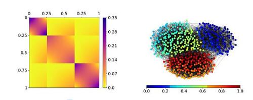
Figure 2 Disjoint univariate linear B-spline bases, colored in blue, orange, green, and red, respectively. Applying the tensor product yields the basis to construct blockwise independent B-spline functions for approaching SBSGMs. Note that this illustration shows the special case of equal community proportions.
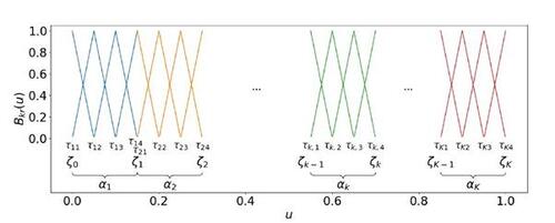
Figure 3 Adjustment of the distribution of the Ui
’s and the community boundaries. Top: Three distributions for the latent quantities which are equivalent in terms of representing the same data-generating process (under applying transformation (11) to accordingly). The solid line represents the density f(u), while the dashed line illustrates the frequency density over the communities, i.e.
. Bottom: Implementation of the adjustment in the algorithm with regard to the empirical cumulative distribution function (including the realizations of
as vertical bars at the bottom). The gray star illustrates the proportion of the two communities against the community boundary.
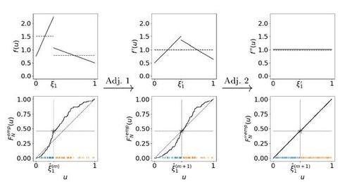
Figure 4 Estimation result for the synthetic SBSGM from Figure 1 (shown again at top left, rescaled according to the estimate’s range from 0 to 0.45). The top right plot illustrates the final estimate of , i.e. after convergence of the algorithm. The estimation is based on the simulated network of size N = 500 at the bottom left, where nodes are colored according to
. A comparison between the simulated Ui
’s and their estimates is illustrated at the bottom right.
![Figure 4 Estimation result for the synthetic SBSGM from Figure 1 (shown again at top left, rescaled according to the estimate’s range from 0 to 0.45). The top right plot illustrates the final estimate of wζ(·,·), i.e. after convergence of the algorithm. The estimation is based on the simulated network of size N = 500 at the bottom left, where nodes are colored according to Ûi∈[0,1]. A comparison between the simulated Ui ’s and their estimates is illustrated at the bottom right.](/cms/asset/4d6cf581-7cb2-4c94-a22a-a0837f50bb8e/ucgs_a_2374571_f0004.jpg)
Figure 5 Estimation results for two synthetic SBSGMs, (a) and (b). (a2) is equivalent to (a), meaning these are two different model representations (with different numbers of groups) for the same data-generating process. Corresponding estimates with number of groups adopted from the model representations above are illustrated in the lower row, denoted by ( ), (
), and (
), respectively. The estimation is based on simulated networks of size N = 500.
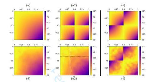
Figure 6 SBSGM estimation on the political blog network. Manually labeled political orientations (see Adamic and Glance, 2005) are illustrated in the top plot. The estimate of (in log scale) is depicted at the bottom left. The node colors in the bottom right plot represent the inferred node positions
.
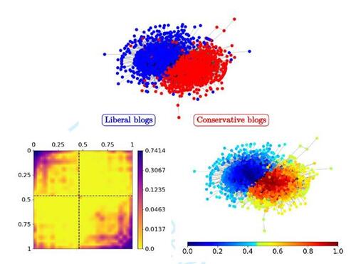
Figure 7 SBSGM estimation on the human brain functional coactivation network (top right, coloring referring to ). The estimate of
(in log scale) is depicted at the top left. The three bottom plots show the local positions of the human brain regions in anatomical space (from left to right: side, front, and top view) with coloring referring to
.
![Figure 7 SBSGM estimation on the human brain functional coactivation network (top right, coloring referring to Ûi∈[0,1]). The estimate of wζ(·,·) (in log scale) is depicted at the top left. The three bottom plots show the local positions of the human brain regions in anatomical space (from left to right: side, front, and top view) with coloring referring to Ûi∈[0,1].](/cms/asset/0b6b74d8-12b5-442b-999f-afd3a40e1e6b/ucgs_a_2374571_f0007.jpg)
Figure 8 Top plot: root-mean-square error between true underlying and inferred edge probabilities based on indicated modeling frameworks. Results refer to the simulation scenarios from Section 4.1 with simulated networks of size N = 500. Bottom row: precision-recall curves for real-world networks from Section 4.2. Predictions refer to network entries that have been randomly modified to imitate unstructured noise. Proportions of (potentially) modified entries are 10% for political blog and human brain network and 30% for military alliance network. Values given in the legend (square brackets) declare the area under the curve. Dashed purple line illustrates result under random classifier.
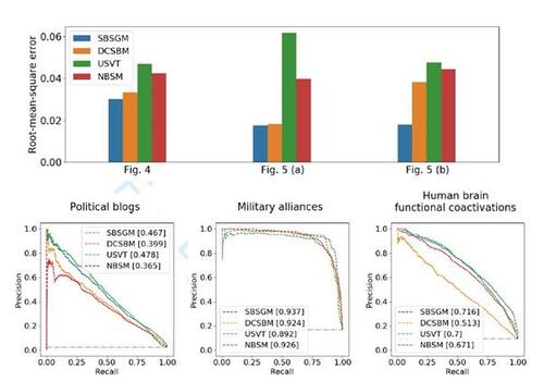
Figure 9 Pareto front with respect to accuracy and run time for all three real-world examples, cf. legend (axes in log scale). Corner points are labeled by associated methods. Dashed lines integrate results that are not part of the Pareto front. Values on the vertical axis correspond to the results depicted in the bottom row of Figure 8.
Supp_Mat_for_SBSGM.pdf
Download PDF (2.1 MB)References
- Adamic, L. A. and N. Glance (2005). The political blogosphere and the 2004 U.S. Election: Divided they blog. In 3rd International Workshop on Link Discovery, LinkKDD 2005 - in conjunction with 10th ACM SIGKDD International Conference on Knowledge Discovery and Data Mining, pp. 36–43.
- Airoldi, E. M., D. M. Blei, S. E. Fienberg, and E. P. Xing (2008). Mixed membership stochastic blockmodels. Journal of Machine Learning Research 9, 1981–2014.
- Airoldi, E. M., T. B. Costa, and S. H. Chan (2013). Stochastic blockmodel approximation of a graphon: Theory and consistent estimation. In Advances in Neural Information Processing Systems 26, pp. 692–700.
- Andersen, M., J. Dahl, and L. Vandenberghe (2016). CvxOpt: Open source software for convex optimization (Python). Available online: https://cvxopt.org [accessed 11-27-2020]. Version 1.2.7.
- Bickel, P., D. Choi, X. Chang, and H. Zhang (2013). Asymptotic normality of maximum likelihood and its variational approximation for stochastic blockmodels. Annals of Statistics.
- Borgs, C., J. Chayes, and L. Lovász (2010). Moments of two-variable functions and the uniqueness of graph limits. Geometric and Functional Analysis 19 (6), 1597–1619.
- Borgs, C., J. Chayes, L. Lovász, V. T. Sós, and K. Vesztergombi (2007). Counting graph homomorphisms. In Topics in Discrete Mathematics, pp. 315–371.
- Burnham, K. and D. Anderson (2002). Model selection and multimodel inference: A practical information-theoretic approach. (2nd ed.). New York: Springer.
- Burnham, K. P. and D. R. Anderson (2004). Multimodel inference: Understanding AIC and BIC in model selection. Sociological Methods and Research 33 (2), 261–304.
- Chan, S. H. and E. M. Airoldi (2014). A consistent histogram estimator for exchangeable graph models. In 31st International Conference on Machine Learning, ICML 2014.
- Chatterjee, S. (2015). Matrix estimation by universal singular value thresholding. Annals of Statistics 43 (1), 177–214.
- Chen, K. and J. Lei (2018). Network cross-validation for determining the number of communities in network data. Journal of the American Statistical Association 113 (521), 241–251.
- Choi, D. S., P. J. Wolfe, and E. M. Airoldi (2012). Stochastic blockmodels with a growing number of classes. Biometrika 99 (2), 273–284.
- Côme, E. and P. Latouche (2015). Model selection and clustering in stochastic block models based on the exact integrated complete data likelihood. Statistical Modelling 15 (6), 564–589.
- Crossley, N. A., A. Mechelli, P. E. Vértes, T. T. Winton-Brown, A. X. Patel, C. E. Ginestet, P. McGuire, and E. T. Bullmore (2013). Cognitive relevance of the community structure of the human brain functional coactivation network. Proceedings of the National Academy of Sciences of the United States of America 110 (28), 11583–11588.
- Daudin, J. J., F. Picard, and S. Robin (2008). A mixture model for random graphs. Statistics and Computing 18 (2), 173–183.
- De Nicola, G., B. Sischka, and G. Kauermann (2022). Mixture models and networks: The stochastic blockmodel. Statistical Modelling 22 (1–2), 67–94.
- Decelle, A., F. Krzakala, C. Moore, and L. Zdeborová (2011). Asymptotic analysis of the stochastic block model for modular networks and its algorithmic applications. Physical Review E - Statistical, Nonlinear, and Soft Matter Physics 84 (6).
- Diaconis, P. and S. Janson (2007). Graph limits and exchangeable random graphs. arXiv preprint arXiv:0712.2749.
- Eilers, P. H. and B. D. Marx (1996). Flexible smoothing with B-splines and penalties. Statistical Science 11 (2), 89–102.
- Fienberg, S. E. (2012). A brief history of statistical models for network analysis and open challenges. Journal of Computational and Graphical Statistics 21 (4), 825–839.
- Fosdick, B. K., T. H. McCormick, T. B. Murphy, T. L. J. Ng, and T. Westling (2019). Multiresolution network models. Journal of Computational and Graphical Statistics 28 (1), 185–196.
- Gao, C., Y. Lu, and H. H. Zhou (2015). Rate-optimal graphon estimation. Annals of Statistics 43 (6), 2624–2652.
- Gao, C. and Z. Ma (2020). Discussion of ’Network cross-validation by edge sampling’. Biometrika 107 (2), 281–284.
- Geng, J., A. Bhattacharya, and D. Pati (2019). Probabilistic Community Detection With Unknown Number of Communities. Journal of the American Statistical Association 114 (526), 893–905.
- Ghasemian, A., H. Hosseinmardi, A. Galstyan, E. M. Airoldi, and A. Clauset (2020). Stacking models for nearly optimal link prediction in complex networks. Proceedings of the National Academy of Sciences of the United States of America 117 (38), 23393–23400.
- Goldenberg, A., A. X. Zheng, S. E. Fienberg, and E. M. Airoldi (2009). A survey of statistical network models. Foundations and Trends in Machine Learning 2 (2), 129–233.
- Handcock, M. S., A. E. Raftery, and J. M. Tantrum (2007). Model-based clustering for social networks. Journal of the Royal Statistical Society. Series A: Statistics in Society 170 (2), 301–354.
- Hoff, P. D. (2007). Modeling homophily and stochastic equivalence in symmetric relational data. In Advances in Neural Information Processing Systems 20 - Proceedings of the 2007 Conference.
- Hoff, P. D. (2009). Multiplicative latent factor models for description and prediction of social networks. Computational and Mathematical Organization Theory 15 (4), 261–272.
- Hoff, P. D. (2021). Additive and multiplicative effects network models. Statistical Science 36 (1), 34–50.
- Hoff, P. D., A. E. Raftery, and M. S. Handcock (2002). Latent space approaches to social network analysis. Journal of the American Statistical Association 97 (460), 1090–1098.
- Holland, P. W., K. Laskey, and S. Leinhardt (1983). Stochastic blockmodels: First steps. Social Networks 5, 109–137.
- Hunter, D. R., P. N. Krivitsky, and M. Schweinberger (2012). Computational statistical methods for social network models. Journal of Computational and Graphical Statistics 21 (4), 856–882.
- Hurvich, C. M. and C. L. Tsai (1989). Regression and time series model selection in small samples. Biometrika 76 (2), 297–307.
- Jaewon, C., D. Pedigo Benjamin, W. Bridgeford Eric, K. Varjavand Bijan, S. Helm Hayden, and T. Vogelstein Joshua (2019). GraSPy: Graph statistics in Python. Journal of Machine Learning Research 20 (158), 1–7.
- Karrer, B. and M. E. Newman (2011). Stochastic blockmodels and community structure in networks. Physical Review E - Statistical, Nonlinear, and Soft Matter Physics 83 (1).
- Kauermann, G. and J. D. Opsomer (2011). Data-driven selection of the spline dimension in penalized spline regression. Biometrika 98 (1), 225–230.
- Kemp, C., J. B. Tenenbaum, T. L. Griffiths, T. Yamada, and N. Ueda (2006). Learning systems of concepts with an infinite relational model. In Proceedings of the National Conference on Artificial Intelligence, Volume 1, pp. 381–388.
- Klopp, O., A. B. Tsybakov, and N. Verzelen (2017). Oracle inequalities for network models and sparse graphon estimation. Annals of Statistics 45 (1), 316–354.
- Kolaczyk, E. D. (2009). Statistical analysis of network data. New York: Springer.
- Kolaczyk, E. D. (2017). Topics at the frontier of statistics and network analysis. Cambridge: Cambridge University Press.
- Kolaczyk, E. D. and G. Csardi (2014). Statistical analysis of network data with R (2nd ed.). New York: Springer.
- Latouche, P. and S. Robin (2016). Variational Bayes model averaging for graphon functions and motif frequencies inference in W-graph models. Statistics and Computing 26 (6), 1173–1185.
- Levine, R. A. and G. Casella (2001). Implementations of the Monte Carlo EM algorithm. Journal of Computational and Graphical Statistics 10 (3), 422–439.
- Li, T. and C. M. Le (2023). Network estimation by mixing: Adaptivity and more. Journal of the American Statistical Association. [Available online.] DOI: 10.1080/01621459.2023.2252137.
- Li, T., E. Levina, and J. Zhu (2020). Network cross-validation by edge sampling. Biometrika 107 (2), 257–276.
- Li, T., E. Levina, J. Zhu, and C. M. Le (2021). randnet: Random network model estimation, selection and parameter tuning (R). Available online: https://mran.microsoft.com/snapshot/2021-08-04/web/packages/randnet [accessed 11-22-2022]. Version 0.4.
- Li, Y., X. Fan, L. Chen, B. Li, and S. A. Sisson (2022). Smoothing graphons for modelling exchangeable relational data. Machine Learning 111 (1), 319–344.
- Lloyd, J. R., P. Orbanz, Z. Ghahramani, and D. M. Roy (2012). Random function priors for exchangeable arrays with applications to graphs and relational data. In Advances in Neural Information Processing Systems, Volume 2, pp. 998–1006.
- Lovász, L. and B. Szegedy (2006). Limits of dense graph sequences. Journal of Combinatorial Theory. Series B 96 (6), 933–957.
- Lusher, D., J. Koskinen, and G. Robins (2013). Exponential random graph models for social networks: Theory, methods, and applications. Cambridge: Cambridge University Press.
- Ma, Z., Z. Ma, and H. Yuan (2020). Universal latent space model fitting for large networks with edge covariates. Journal of Machine Learning Research 21, 1–67.
- Mariadassou, M., S. Robin, and C. Vacher (2010). Uncovering latent structure in valued graphs: A variational approach. Annals of Applied Statistics 4 (2), 715–742.
- Matias, C. and S. Robin (2014). Modeling heterogeneity in random graphs through latent space models: A selective review. ESAIM: Proceedings and Surveys 47, 55–74.
- McCulloch, C. E. (1994). Maximum likelihood variance components estimation for binary data. Journal of the American Statistical Association, 330–335.
- Newman, M. E. (2006). Modularity and community structure in networks. Proceedings of the National Academy of Sciences of the United States of America 103 (23), 8577–8582.
- Newman, M. E. and G. Reinert (2016). Estimating the number of communities in a network. Physical Review Letters 117 (7).
- Nowicki, K. and T. A. Snijders (2001). Estimation and prediction for stochastic blockstructures. Journal of the American Statistical Association 96 (455), 1077–1087.
- Olhede, S. C. and P. J. Wolfe (2014). Network histograms and universality of blockmodel approximation. Proceedings of the National Academy of Sciences 111 (41), 14722–14727.
- Orbanz, P. and D. M. Roy (2015). Bayesian models of graphs, arrays and other exchangeable random structures. IEEE Transactions on Pattern Analysis and Machine Intelligence 37 (2), 437–461.
- Peixoto, T. P. (2012). Entropy of stochastic blockmodel ensembles. Physical Review E - Statistical, Nonlinear, and Soft Matter Physics 85 (5).
- Peixoto, T. P. (2017). Nonparametric Bayesian inference of the microcanonical stochastic block model. Physical Review E - Statistical, Nonlinear, and Soft Matter Physics 95 (1).
- Riolo, M. A., G. T. Cantwell, G. Reinert, and M. E. Newman (2017). Efficient method for estimating the number of communities in a network. Physical Review E - Statistical, Nonlinear, and Soft Matter Physics 96 (3).
- Rohe, K., S. Chatterjee, and B. Yu (2011). Spectral clustering and the high-dimensional stochastic blockmodel. Annals of Statistics 39 (4), 1878–1915.
- Rubinov, M. and O. Sporns (2010). Brain connectivity toolbox (MATLAB). Available online: https://sites.google.com/site/bctnet [accessed 02-15-2021].
- Ruppert, D., M. P. Wand, and R. J. Carroll (2003). Semiparametric Regression. Cambridge: Cambridge University Press.
- Ruppert, D., M. P. Wand, and R. J. Carroll (2009). Semiparametric regression during 2003–2007. Electronic Journal of Statistics 3, 1193–1256.
- Salter-Townshend, M., A. White, I. Gollini, and T. B. Murphy (2012). Review of statistical network analysis: Models, algorithms, and software. Statistical Analysis and Data Mining 5 (4), 243–264.
- Schweinberger, M. and M. S. Handcock (2015). Local dependence in random graph models: Characterization, properties and statistical inference. Journal of the Royal Statistical Society. Series B: Statistical Methodology 77 (3), 647–676.
- Sischka, B. (2022). EM-based estimation of stochastic block smooth graphon models (Python). Available online: https://github.com/BenjaminSischka/SBSGMest.git [accessed 03-24-2022].
- Sischka, B. and G. Kauermann (2022). EM-based smooth graphon estimation using MCMC and spline-based approaches. Social Networks 68, 279–295.
- Snijders, T. A. (2011). Statistical models for social networks. Annual Review of Sociology 37, 131–153.
- Snijders, T. A. and K. Nowicki (1997). Estimation and prediction for stochastic blockmodels for graphs with latent block structure. Journal of Classification 14 (1), 75–100.
- Turlach, B. A. and A. Weingessel (2013). quadprog: Functions to solve quadratic programming problems (R). Available online: https://CRAN.R-project.org/package=quadprog [accessed 11-27-2020]. Version 1.5-5.
- Wang, Y. X. and P. J. Bickel (2017). Likelihood-based model selection for stochastic block models. Annals of Statistics 45 (2), 500–528.
- Wei, G. C. G. and M. A. Tanner (1990). A Monte Carlo implementation of the EM algorithm and the poor man’s data augmentation algorithms. Journal of the American Statistical Association, 699–704.
- Wolfe, P. J. and S. C. Olhede (2013). Nonparametric graphon estimation. arXiv preprint arXiv:1309.5936.
- Wood, S. N. (2017). Generalized additive models: An introduction with R (2nd ed.). Boca Raton: CRC Press.
- Yang, J. J., Q. Han, and E. M. Airoldi (2014). Nonparametric estimation and testing of exchangeable graph models. In Proceedings of the Seventeenth International Conference on Artificial Intelligence and Statistics. Journal of Machine Learning Research, Conference and Workshop Proceedings 33, PMLR, pp. 1060–1067.
- Zhang, Y., E. Levina, and J. Zhu (2017). Estimating network edge probabilities by neighbourhood smoothing. Biometrika 104 (4), 771–783.