An inverse boundary element method/genetic algorithm based approach for retrieval of multi-dimensional heat transfer coefficients within film cooling holes/slots

Abstract

An inverse methodology is developed as a means of determining heat transfer coefficient distributions in film cooling holes/slots. Thermal conditions are over-specified at exposed surfaces amenable to measurement, while the temperature and surface heat flux distributions are unknown at the film cooling hole/slot walls. The latter are determined in an iterative manner by solving an inverse problem whose objective is to adjust the film-cooling hole/slot wall temperatures and heat flux distributions until the temperature and heat fluxes at the measurement surfaces are matched in an overall heat conduction solution. The heat conduction problem is solved using boundary element methods, and the inverse problem is solved using a genetic algorithm. The resulting film coefficient distributions are fit to a correlation reflecting dependency on position, the Prandtl and Reynolds numbers.

1. Introduction

Given the large number of sustained operational hours required for industrial turbines, two important demands placed on such engines are component life and overall engine performance. These demands are somewhat conflicting because high temperatures are required at the inlet to the turbine in order to achieve high efficiency; however, increasing inlet turbine temperature in turn causes reduced component life. One way to overcome this problem is to employ film cooling. Film cooling is the introduction of a secondary fluid (coolant or injected fluid) at one or more discrete locations along a surface exposed to a high temperature environment to protect that surface not only in the immediate region of injection but also in the downstream region [1]. To define film cooling effectiveness (η), the surface temperature downstream of the cooling slot is to be measured or computed. An expression often used for compressible flow film cooling [1] is: (---79--1) where T is the measured temperature downstream of the cooling slot, T_oc is the stagnation temperature of the cooling fluid at the point of injection, and T_r is the recovery temperature of the hot gas. The recovery temperature can be defined as the fluid bulk temperature, or the adiabatic wall temperature. It is important to characterize the efficacy of such a cooling scheme, particularly as the compressor air employed to protect critical parts of the turbine is very expensive from an overall engine performance perspective. The film effectiveness is a common way to report the adiabatic wall temperature that is the driving temperature for the convection at the exposed metal surfaces and to simultaneously provide a measure of the efficacy of film-cooling scheme. The film effectiveness can be measured in carefully designed experiments. However, in determining the film coefficient distributions at the exposed surfaces, the distributions of thermal conditions within the cooling holes/slots are unknown. As there are no correlations or experimental data in the open literature available to characterize an accurate heat flux distribution in such cases, there exists a need to determine the film coefficient distributions in film cooling holes/slots.

Film cooling configurations have been investigated for several years. Concerning the CFD research on this subject, a bibliography (1971–1996) of the most important publications can be found in a study by Kercher [2]. There have been different studies that have measured endwall heat transfer and film cooling characteristics as a result of injection from a two-dimensional flush slot just upstream of the vane [3–6]. On the three-dimensional film cooling side, most of the published work on predictions of film cooling is based on either a parabolic or semielliptic procedure. Goldstein et al. [7, 8] studied the effect of cooling holes on turbine vanes and blades. Recent numerical studies on the leading edge film-cooling physics [9, 10] focused on the determination of the adiabatic film cooling effectiveness and heat transfer coefficients.

In several industrial applications, it is necessary to accompany the computation of the flow and associated heat transfer in the fluid with the heat conduction inside the adjacent solid surfaces. The coupling of these two modes of heat transfer has been identified by the name ‘conjugate heat transfer' in the literature. Several researchers have investigated coupled conjugate heat transfer analysis. Some of them presented a coupled scheme between the finite-volume-based Navier–Stokes solver and the finite-element-based program for heat conduction [11]; others used the finite-volume based code ‘Fluent 5’ [12]. Whereas other researchers pursued a different method of coupling the fluid and solid thermal problems: the basis for their technique is the Boundary Element Methods (BEM) for the solution of solid conduction problem. Since the thermal conduction in the solid is governed by Laplace equation for temperature, it may be solved using only boundary discretization [13].

Retrieval of surface heat flux or convection heat transfer coefficient h is often accomplished using surface temperature histories provided by thermographic techniques applied in controlled experiments and in conjunction with theoretical assumptions. It is herein proposed to use the BEM to resolve 2D and 3D heat transfer and determine h by inverse methods. The BEM is ideally suited for this inverse problem as surface temperatures and fluxes appear as nodal unknowns. These are precisely the variables required in inverse analysis. Surface fluxes have been retrieved using BEM-based inverse algorithms and internal temperature measurements: see Kurpisz and Nowak [14]. In a numerical study, Maillet et al. [15] formulated an inverse BEM-based approach to retrieve angular distributions of h from a cylinder using second order regularization to stabilize results. Farid and Hsieh [16] used an inverse BEM approach to retrieve angular variation of h over a rough heated horizontal cylinder in an experiment where steady-state surface temperatures are measured nonintrusively by infrared scanning. Martin and Dulikravich [17] used a steady-state BEM-based approach in a numerical study to retrieve h and Singular Value Decomposition to stabilize results. Kassab et al. [18] and Divo et al. [19] developed a BEM-based inverse algorithm to retrieve multidimensional varying h from transient surface temperature measurements. At each time level, a regularized functional is minimized to retrieve current heat fluxes and simultaneously smooth out the effect of measurement errors. Kassab et al. [20–22] developed an inverse algorithm to reconstruct multidimensional surface heat flux, and minimized the functional using the Levenberg–Marquardt method and Genetic Algorithms (GAs). They showed that GAs can be used successfully to retrieve surface heat flux distributions.

From the literature reviewed above, it is clear that although film cooling has been studied extensively, there is a lack of information with regard to the thermal conditions within the film hole/slot itself. The purpose of this paper is to develop an inverse methodology as a means of determining the distributions of heat transfer coefficient in film cooling holes/slots. Thermal conditions are overspecified at exposed surfaces amenable to measurement, while the temperature and surface heat flux are unknown at the film cooling hole/slot walls. The latter are determined in an iterative manner by solving an inverse problem whose objective is to adjust the film-cooling hole/slot wall temperatures and heat fluxes until the temperature and heat flux at the measurement surfaces are matched in an overall heat conduction solution. The heat conduction problem is solved using boundary elements, and the inverse problem is solved using a genetic algorithm. The resulting film coefficient distribution is fit to a correlation reflecting dependency on position, the Prandtl and Reynolds numbers.

2. Inverse problem methodology for film coefficient reconstruction

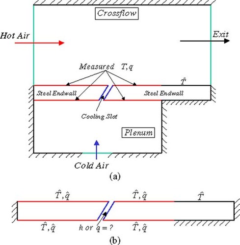
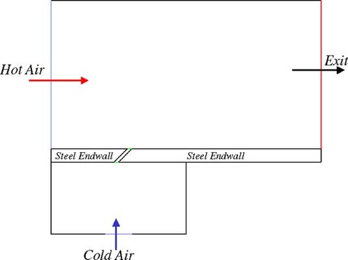
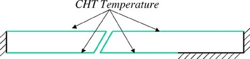
The inverse problem approach to film coefficient reconstruction is developed here. Consider the specific case of a 2D film cooling slot supplied by a plenum, see figure 1(a). This configuration is used here for illustration in the development of the inverse problem methodology. The model consists of the domain of the main flow (hot gas), the coolant plenum supply (cold gas), and the endwall with a cooling slot of specified injection angle. The outlet was located far downstream of the cooling slot. The measured temperature and heat flux over specified surfaces as shown in figure 1(b) will be used as an input for the inverse problem to determine the unknown temperature and heat flux in the cooling slot. The heat flux will be measured using an optical thermographic technique under development at the University of Central Florida. The inverse problem algorithm developed herein for the reconstruction of heat transfer coefficient distributions is comprised of an objective function to be minimized; i.e. root mean square (RMS) error in heat flux, a minimization algorithm; i.e. genetic algorithm, and a forward problem field solver; i.e. BEM. Each of these will be discussed in detail in the following sections.

Figure 1. Schematic for the Inverse Problem applied to a slot cooling configuration. (a) overall configuration; (b) domain of the inverse conduction problem.

2.1 The objective function and regularization

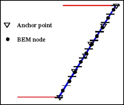
The objective of the inverse problem under consideration is to reconstitute the heat transfer coefficients or heat flux, h or q, at the cooling slot/hole. Here, Cauchy conditions imposed at the surfaces exposed to the hot gases and to the film cooling supply plenum, as shown in figure 1(b). These surfaces are referred from here on as measurement surfaces. This is due to the fact that the heat flux and temperature are to be simultaneously measured in order to specify the Cauchy conditions required to solve the inverse problem. In the inverse problem, the temperature is imposed at these surfaces and an initial heat flux distribution is guessed at the cooling slot walls. A forward steady-state heat conduction problem is solved using the BEM, and an objective function is defined to quantify the difference between the heat flux measured at the exposed surfaces and the heat flux predicted by the BEM under current heat flux estimates at the cooling slot surfaces. In order to reduce the number of unknowns, the heat fluxes are parametrically represented using radial basis functions (RBF) [23, 24] as follows, see figure 2: (---79--2) where, N_A is the number of anchor points, (---79----1) is the position vector(---79----2) is the position vector pointing to the jth anchor point, and the expansion coefficients (---79----3) are found through a collocation procedure. The conic RBF, (---79----4) , used in this expansion is (---79--3) Collocating at all the j = 1,2, …, N_A anchor points, there arises a linear equation (---79--4) where(---79----5) is an interpolant matrix. This linear system is solved by standard methods for the expansion coefficients (---79----6) .

Figure 2. Schematic diagram for anchor points using RBF.

Subsequently, the following objective function is defined to measure the difference between the BEM-computed heat flux, q_BEMi (---79----7) , at the i=1,2,…, N_m, measuring points and the measured heat flux (---79----8) at the measuring points under the current estimate of (---79----9) : (---79--5) As has been discussed, inverse problems are ill-posed and small errors in inputs are reflected in large errors in output unless regularization (a form of stabilization) or a stabilizing inverse problem solver is adopted. In this work, the objective functional is therefore regularized using a first order method [18, 19] as (---79--6) where, (---79----10) is heat flux at the anchor points, and (---79----11) is least-square curve fitted heat flux through the anchor points. In general, the number of anchor points (N_A) is less than the number of measuring points (N_m), and the number of anchor points is chosen in a manner to obtain a converged solution in the sense of small variations in the heat flux distributions as the number of anchor points is varied. The regularization parameter, β, can take on values from zero (no regularization) to an appropriate positive number. The choice of optimal β is the subject of much research in the inverse problem community. For example, β may be chosen via the L-curve method [25, 26] or the discrepancy principle [27, 28]. In this work, the optimal β has been determined by constructing a plot of β versus the best fitness, (---79----12) . The process starts by setting β to zero which results in the maximum best fitness, then β is increased until the reconstructed heat fluxes manifest no oscillatory behavior. At this point, if two lines are drawn from the two extreme ends, we take value of β at the point of intersection.

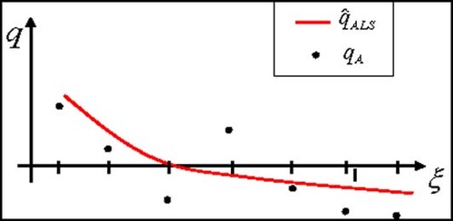
The mean values of the heat fluxes at the anchor points (---79----13) are obtained by least-squares fitting a quadratic or higher order polynomial through the anchor point values (---79----14) , see figure 3: (---79--7) where(---79----15) is the coefficient matrix of the normal equations, and its dimension is equal to the number of anchor points. The regularization has the effect of drawing the current flux distribution towards its current mean value. Obviously, the amount of stabilization depends on the value of β.

Figure 3. Schematic diagram for the least square curve fitting of the heat fluxes at the anchor points.

2.2 The genetic algorithm

The GA optimization process begins by setting a random set of possible solutions, called the population, with a fixed initial size or number of individuals. Each individual is defined by optimization variables and is represented as a bit string or a chromosome; see figure 4. A GA iteratively alters the heat flux distribution at the cooling slot walls until the measured surface heat fluxes are matched thus, satisfying the Cauchy conditions at the exposed measuring surfaces. It should be noted that GAs maximize objective function as they naturally seek the ‘best fit’ [29]. Thus the objective function computed by the GA is actually, (---79--8) The objective function, (---79----16) , is evaluated for every individual in the current population defining the fitness or their probability of survival. At each iteration of the GA, the processes of selection, cross-over, and mutation operators are used to update the population of designs. A selection operator is first applied to the population in order to determine and select the individuals that are going to pass information in a mating process with the rest of the individuals in the population. This mating process is called the crossover operator, and it allows the genetic information contained in the best individuals to be combined to form offsprings. Additionally, a mutation operator randomly affects the information obtained by the mating of individuals. This is a crucial step for continuous improvement.

Figure 4. Example of an individual in the population characterized by four parameters (genes) encoded in a chromosome yielding the individuals's fitness value F₁.

A series of parameters are initially set in the GA code, and these determine and affect the performance of the genetic optimization process. The number of parameters per individual or optimization variables, the size of the bit string or chromosome that defines each individual, the number of individuals or population size per generation, the number of children from each mating, the probability of crossover, and the probability of mutation are among the parameters that control the optimization process. This set of operations is carried out generation after generation until either a convergence criterion (a preset level of acceptable fitness) is satisfied or a maximum number of generations is reached. It is also important to point out that three important features distinguish GAs from the other evolutionary algorithms, namely: (1) binary representation of the solution, (2) the proportional method of selection, and (3) mutation and crossover as primary methods of producing variations.

In nature, the properties of an organism are described by a string of genes in the chromosomes. Therefore, if one is trying to simulate nature using computers one must encode the design variable in a convenient way. We adopt a haploid model using a binary vector to model a single chromosome. The length of the vector is dictated by the number of design variables and the required precision of each design variable. Each design variable has to be bounded by a minimum and a maximum value and in the process the precision of the variable is determined. The number of divisions used in the discretization has to be an integral power of two. This procedure allows an easy mapping from real numbers to binary strings and vice versa. This coding process represented by a binary string is one of the distinguishing features of GAs and differentiates them from other evolutionary approaches. The haploid GAs place all design variables into one binary string, called a chromosome or off-spring. The information contained in the string of vectors comprising the chromosome characterizes an individual in a population. In turn, each individual is equipped with a given set of design variables to which corresponds a value of the objective function. This value is the measure of “fitness” of the individual design. In GAs, poorly fit designs are not discarded, rather they are kept, as in nature, to provide genetic diversity in the evolution of the population. This genetic diversity is required to provide forward movement of the population during the mating, crossover, and mutation processes which characterize the GA.

The initial population size may grow or diminish to mimic actual biological systems. However, in the GA used here, the population size is not allowed to change while the program is running. Once the population size is fixed, the algorithm initializes all of the chromosomes. This operation is carried out by assigning a random value of 0 or 1 for each bit contained in each of the chromosomes. After initializing the population, evaluation of the fitness of each individual is performed by computing the objective (or fitness) which, of course, represents a set of possible solutions. Having the values of the objective function for each individual, the selection process can be started. First values of the fitness function for each individual have to be added, and then the probability of being a selected individual is calculated as the ratio between the value of the fitness function of each individual and the sum of all objectives function values. This is given by: (---79--9) where v_i is the ith member of the population, and Fitness(v_i) is the measure of the fitness of that member under its currently evolved parameter set configuration. A weighted roulette wheel is generated, where each member of the current population is assigned a portion of the wheel in proportion to its probability of selection. The wheel is spun as many times as there are individuals in the population to select which members mate. Obviously, some chromosomes would be selected more than once, where the best chromosomes get more copies, the averages stay even, and the worst die off. Once selection has been applied, crossover and mutation occur in the surviving individuals. These operations further expand genetic diversity in the current population. All other probabilities referred to in the description of the GA adopted in this paper are computed in an analogous fashion to the selection probability.

The probability of crossover P_c is an important parameter that defines the expected population size (P_c • pop−size) of chromosomes which undergoes crossover operation. This is a mating process that allows individuals to interchange intrinsic information contained in the chromosomes. The operation may be implemented in two steps: (1) a random selection based on the probability of crossover is performed to obtain pairs of individuals, and (2) a random number is generated between the first position of the binary vector and the last one to indicate the location of the crossing point which delineates the location about which genetic information is interchanged between two chromosomes.

The mutation operator is the final operator implemented. The probability of mutation P_m gives the expected number of mutated bits and every bit in all chromosomes in the whole population has an equal chance to undergo mutation: switch of a bit from 0 to 1 or vice-versa. This process is implemented by generating a random number within the range (0 … 1) for each bit within the chromosome. If the generated number is smaller than P_m the bit is mutated. When the mutation is done on a bit-by-bit basis it is called the creep mutation. Another type of mutation is the jump mutation which is applied to an individual selected to be mutated from this perspective. In this case all bits within the chromosome are switched from 0 to 1 and vice-versa. Following selection, crossover, and mutation the new population is ready for its next evolution until the convergence criteria “fitness” is reached. It is the very nature of the binary representation of the design variables of the objective function and the random search process which provide yet another but implicit degree of regularization in this optimization process. The sensitivity of the objective function can be tuned depending on the size of each element of the chromosome. Thus, low bit representation is insensitive to large variations in input (regularized but may lead to a poor solution due to low resolution), while high bit representation is sensitive to large variations in the input (not regularized and therefore may lead to a poor solution as well). There is a range of bit size which produces a regularized and sensitive response leading to stable solutions.

The following parameters are chosen to generate results: population size of 50 individuals/generation, a string of eight bits to define each parameter within each individual, one child per mating, a 4% probability of mutation, a 20% probability of creep mutation, and a 50% probability of crossover. This combination of parameters and procedures has been proven to yield efficient and accurate optimization results for different studies carried out in this article.

2.3 The forward boundary element method heat conduction solver

The BEM is used to solve the forward problem. This technique is based on integral equation formulations and is ideally suited for the problem under consideration as it requires only a boundary mesh for steady linear or nonlinear heat conduction and the nodal unknowns appearing in the equations are the temperature and heat flux. The governing equation for steady state heat conduction with constant conductivity and no internal generation is the Laplace equation for the temperature: ∇²T=0. An integral equation (BIE) for the temperature is readily derived as [10]: (---79--10) where C(ξ) is one for a source point at the interior and 1/2 for a source point on a smooth boundary, S(x) is the surface bounding for the domain of interest, ξ is the source point, x is the field point, q(x) is the heat flux, T* (x,ξ) is the fundamental solution, and F(x,ξ) is its normal derivative with respect to the outward normal. The integral equation is discretized by introducing a pattern of N-boundary nodes over the surface and boundary elements to model the boundary, temperature, and flux distributions and can be expressed in a standard matrix form as [31–33] (---79--11) The influence coefficient matrices (---79----17) and (---79----18) are evaluated numerically, depending on the type of element chosen and the dimension of the problem. In this article, all computations are carried out in 2D using exclusively discontinuous quadratic isoparametric boundary elements. In this element type, the geometry, temperature and heat flux are modeled using biquadratic shape functions. However, the temperature, and heat flux end-nodes are offset from the geometric end-nodes; see figure 5. Consequently, this type of element is termed discontinuous. It offers the advantage of superior heat flux determination with none of the complexities plaguing continuous elements, in particular in 3D. Note that the geometric nodal locations of the element are ordered counterclockwise such that the normal vector always points outwards from the domain of the problem, thus uniquely defining the outward normal. The global coordinate system (x,y) is transformed into a local coordinate system (ξ) using quadratic shape functions. The influence coefficients H_ij and G_ij that are elements of the matrices (---79----19) and (---79----20) are defined as integrals over the boundary element Γ_j, (---79--12) and these are evaluated using adaptive quadratures based on Gauss–Kronrod rules. Introducing the boundary conditions, into the discretized BEM equations leads to the standard algebraic form: (---79--13) This equation can be solved by direct methods such as LU decomposition or by iterative methods for nonsymmetric equations such as GMRES.

Figure 5. Discontinuous isoparametric element: quadratic geometry, T and q.

As an example of a BEM mesh, quadratic discontinuous elements have been used to discretize the geometry of interest in this article. A total of 200 elements were used to discrete the whole domain, such that the left block has 60 elements and the right block has 140 elements, and each side of the cooling slot has ten elements. The surface mesh is shown in figure 6 below.

Figure 6. Surface mesh of the direct problem.

3. Conjugate heat transfer simulation (CHT) of a 2D cooling slot

In order to verify the approach developed for the solution of the inverse problem, a numerical simulation will be undertaken specifically considering a 2D cooling slot model. Here, a full conjugate heat transfer analysis will be carried out using Fluent to simulate measurements of temperature and heat flux used to provide over-specified conditions for the inverse problem. Subsequently, these simulated measurements are used to solve the inverse problem of reconstruction of the film coefficient distributions at the cooling slot walls.

The computational model was chosen to simulate an experiment currently underway at the University of Central Florida. The domain of the main flow is 30 × 16.5 cm, the coolant plenum supply is 15 × 8 cm with an inlet of 3 cm. The endwall is 15 mm thick with a cooling slot opening of 5 mm wide and 45° injection angle. The outlet was located far downstream of the cooling slot. A view of the computational domain is shown in figure 7.

Figure 7. Diagram of the CHT computational domain.

A multiblock numerical grid was used in this problem to get a structured mesh in the fluid domain and part of the solid domain. The grid was created in Gambit from Fluent, Inc. Since the enhanced wall functions had been used, the cells in the near-wall layers were stretched away from the surfaces, and all wall-adjacent grid points were located at a y⁺ equal to or less than five. Notice that the enhanced wall functions extend their applicability throughout the near-wall region (i.e., laminar sublayer, buffer region, and fullyturbulent outer region). A view of the computation mesh is shown in figure 8. The mesh has 42,408 cells, with 40,527 cells for the fluid domain, and 1881 cells for the solid domain, i.e. endwall.

Figure 8. View of the CHT computational Grid, (a) whole domain, and (b) close up of the cooling slot.

The conjugate heat transfer CHT simulation conditions were chosen to match the experiment where the air flow is modeled as a compressible flow using the ideal gas law, and the other properties are linear function of temperature. The endwall material is stainless steel, with properties varying as linear function of temperature. A profile for total pressure at the main flow inlet was specified based on the Blasius 1/7th power law turbulent velocity profile. The main flow enters at temperature of 350 K, and free stream turbulence intensity of 3%. The coolant flow enters at temperature of 300 K, and total pressure of 105,800 Pa. Subsequently, the results will be scaled to actual engine conditions using power law type relations. The present simulation employed Re-Normalization Group (RNG) k−ε turbulence model. The solver used in the simulations is the commercial code Fluent 6, from Fluent, Inc.

4. Numerical results

We now present the simulated results in three parts; results of the conjugate heat transfer simulation, results of the direct conduction problem, and results of the inverse problem. The purpose of the CHT simulation is to provide numerical input to the inverse problem. The numerical results simulate measurements. Moreover, the direct conduction problem is carried out to provide a consistency check between the commercial CFD code used in the CHT simulation and the in-house BEM code that is the forward solver for the inverse problem.

4.1 Results of the conjugate heat transfer simulation

The problem has been solved in double precision for the two cases; i.e. conjugate and adiabatic, and the results are convergent at least 10⁻⁵ for all residuals (mass, x and y velocities, energy, k and ε). The velocity and the temperature contours for the conjugate case are shown in figure 9.

Figure 9. Velocity and temperature contours through the cooling slot for the CHT simulation (a) velocity contours; (b) temperature contours.

4.2 Results of direct conduction problem

We establish a solution to the forward problem as a numerical consistency check of the BEM solution (in house) and conjugate heat transfer CHT (commercial) code. Since the BEM surface mesh and CHT surface mesh are different from each other, a radial basis function interpolation approach is used to pass information from one grid to the other. The input to the direct problem is the CHT wall temperatures at solid surfaces, as shown in figure 10, to check consistency in the BEM-computed heat fluxes.

Figure 10. Schematic diagram of the direct problem.

The discretized governing equations with the specified boundary conditions have been solved, and the temperature distribution with the heat flux direction is shown in figure 11. It can be seen that the temperature expands from 295 K to 345 K, which matches the conjugate heat transfer CHT solution very well (see figure 11). The BEM-computed heat fluxes have been compared to the CHT-computed fluxes in figure 12. The two are in good agreement. Note that the CHT model solved the parabolic heat conduction equation up to the steady-state while the BEM solved the elliptic steady conduction solution.

Figure 11. Temperature distribution predicted by the BEM direct solution.

Figure 12. Comparison of direct BEM heat fluxes and CHT heat fluxes through cooling slot, (a) left edge, and (b) right edge.

4.3 Results of the inverse problem

The results of the inverse problem are now presented for several cases. First, we consider the case of exact input data. The problem has been solved for two blocks: the first one represents the left edge of the cooling slot, this block has 60 elements, and the elements of the cooling slot are 21–30. The second block represents the right edge of the cooling slot: it has 140 elements, and the cooling slot elements are 61–70, as shown in the figure 13 below. The problem has been solved with 21 anchor points. The results for the reconstructed heat fluxes at the left and right edges of the cooling slot are plotted in figure 14. Here the results are shown at zero regularization with 7th order polynomial least-squares fit. The 7th order polynomial was chosen to obtain the best fit in (---79----21) without introducing oscillations in the functional approximations. An initial guess of q between 0–15 kW/m² at the left edge and 0–2 kW/m² at the right edge is taken at all anchor points to begin the minimization process in all cases.

Figure 13. Reference node numbering for the BEM discretization of the inverse problem.

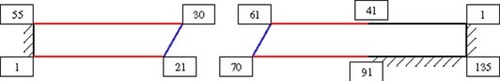
Figure 14. BEM retrieved q through cooling slot at: (a) left edge and (b) right edge. Regularization parameter: β =0.

Figure 15 shows best fitness as function of regularization/tuning parameter. In this figure, the process started with zero regularization which gives the maximum best fitness, then the regularization parameter is increased until the reconstructed heat fluxes manifest no oscillatory behavior. If two lines are drawn from the two extreme ends, the optimal value of β is found at the point of intersection; in this case the best fitness was at a regularization parameter of 10⁻⁷ for the left edge and 10⁻⁵ for the right edge, and as a result, the reconstructed heat fluxes matched the measured ones as shown in figures 16 and 17.

Figure 15. Plot of the regularization parameter β versus the best fitness, (a) left edge and, (b) right edge.

Figure 16. Comparison of reconstructed regularized GA and CHT heat fluxes at: (a) left block (β = 10⁻⁷) and (b) right block (β = 10⁻⁵).

Figure 17. Close up of reconstructed regularized GA and CHT heat fluxes through cooling slot at: (a) left edge (β = 10⁻⁷) and (b) right edge (β = 10⁻⁵).

Next, results are presented for the case of error-laden inputs. Here, a random number generator is employed to generate random errors of maximum levels ±0.5°C in the temperature, and ± 50 W/m² in the heat flux. The results are shown in the figures below. It can be noted that the GA reconstructed heat flux is robust to these random errors yielding very accurate results. The reconstructed heat fluxes at an input error of ± 0.25°C and ± 25 W/m² are shown in figure 18 through left and right sides of the cooling slot, and figure 19 for an input error of ± 0.5°C and ± 50 W/m². It can be seen that the reconstructed and measured heat fluxes are matching each other quite well.

Figure 18. Comparison of reconstructed heat flux using GA-based method with CHT heat fluxes through cooling slot at: (a) left edge (β = 0.1) and (b) right side (β = 0.01). Input Errors: ε_T=±0.25° C, ε_q=±25 W/m².

Figure 19. Comparison of reconstructed heat flux using GA-based method with CHT heat fluxes through cooling slot at: (a) left edge (β = 0.1) and (b) right side (β = 0.01). Input Errors: ε_T=± 0.5° C, ε_q=±50 W/m².

5. Determining a correlation

Once the heat flux is determined, it is the practice in heat transfer to report the result by defining the local film coefficient, h_x, as the local heat flux normalized with respect to an appropriate reference temperature as (---79--14) where h_x is the local heat transfer coefficient (W/m² K), q_w,x is local wall heat flux (W/m²), T_wall,x is local wall temperature (K), and T_ref is a reference temperature (K). The reference temperature can be defined as the fluid bulk temperature, or the adiabatic wall temperature. In our examples, we set the reference temperature equal to the fluid bulk temperature at the cooling slot inlet which is amenable to measurements. (---79--15) The dependency of the local heat transfer coefficient on the relevant dimensionless parameters is readily found from dimensional analysis to be: (---79--16) where Re_x is local Reynolds number, kis thermal conductivity for air (0.026 W/m K), Pr is Prandtl number which is equal to 0.72 for air, D is the diameter of the cooling hole/slot (D=2w), w is the slot width (w=0.0071 m), and Nu_x is local Nusselt number. In our example, the mass flow rate through the cooling slot is (---79----22) , length of the cooling hole/slot (L=0.0212 m), coolant inlet temperature (T_c, _in =297.6 K), and the coolant exit temperature (T_c, _out=295.5 K). The result of curve fitting the local heat transfer coefficient at the left-side of the cooling slot is (see figure 20(a)), (---79--17) and at the other side of the cooling slot; i.e. right side, is given by (see figure 20(b)): (---79--18) It is interesting to compare these results to existing correlations. The Dittus–Boelter equation for constant wall temperature is [34] (---79--19) with n=0.4 for Ts>T_m(heating), and n=0.3 for T_s<T_m (cooling); this formula is applicable for Re_D≥10,000, (L/D)≥10, and 0.7≤ Pr ≤ 160. T_s, T_m are surface and bulk temperature, respectively. It is noted that the above formula tends to over-predict the Nusselt number for gases by at least 20%, and to under-predict Nusselt number for the higher-Prandtl-number fluids by 7–10% [35]. Another formula derived by Kays and Crawford [35] for turbulent flow in a circular tube with fully developed velocity and temperature profiles subjected to a constant wall heat rate is: (---79--20) and for a constant wall temperature, equation (20)(---79--20) can be modified by lowering the coefficient a few percents to yield (---79--21) A comparison in terms of Nusselt number for the average curve fitted heat transfer coefficient at each side and the values predicted by the other correlations is shown in table 1. It can be seen that the average curve fitted Nu_D for both sides is approximately equal to the average Nu_D predicted by Dittus–Boelter and Kays–Crawford correlations for a constant wall temperature, and it is in a better agreement with the average Nu_D predicted by Dittus–Boelter equation for a constant wall temperature and Kays–Crawford correlation for a constant wall heat rate.

Figure 20. Curve fitting the local heat transfer coefficient through cooling slot, (a) left edge, and (b) right edge.

Table 1. Comparison of average Nusselt number.

	(NuD)avg.
Left Side, equation (17)	292.0
Right Side, equation (18)	78.0
Average of left and right sides	185.4
Dittus–Boelter, equation (19)	205.5
Kay and Crawford, equation (20)	168.3
Kay and Crawford modified, equation (21)	160.6
Average of equation (19) and equation (20)	186.9
Average of equation (19) and equation (21)	183.1

6. Conclusions

In this article, we develop an inverse problem approach as a means of determining heat transfer coefficient distributions in film cooling holes/slots. The latter are determined in an iterative manner by solving an inverse problem. The heat conduction problem is solved using boundary element methods, and the inverse problem is solved using a genetic algorithm. It can be noted that the GA reconstructed heat flux is robust yielding very accurate results to both cases; exact input data, and error-laden inputs. The resulting film coefficient distributions are fit to a correlation reflecting dependency on position, the Prandtl and Reynolds numbers.

Acknowledgements

The author would like to thank Dr. L. Elliott and Professor D.B. Ingham from the Department of Applied Mathematics at the University of Leeds for all their encouragement in performing this research work.