Trying To Be Random in Selecting Numbers for Lotto

Abstract

In the lottery game Lotto n/N, the winning n numbers are selected randomly and without replacement from {1, 2, 3, ..., N}. The selection of the winning numbers is normally done with a highly sophisticated mechanical device, and one of the appealing aspects of Lotto is that this procedure is seen to be fair and unbiased. An important perceived consequence is that no one (for a given amount of money) is seen to have a better chance of winning than anyone else. Few people would be willing to let an individual perform this task because of possible bias, but do we really know how difficult it is for an individual to be random in selecting numbers? In an experiment to observe the types and degrees of bias an individual might possess, data were collected from students who were asked to perform as 'random' number generators for the Lotto 6/42 game. Data consisting of the winning numbers from the Irish National Lottery game Lotto 6/42 were obtained from previous years, and a statistical package (in this case, S-Plus) was used to generate other simulated data. A comparison of the three sets of data using many of the basic tools in descriptive statistics together with some goodness of fit tests provides a useful exercise for students to test their intuition about randomness and to discover some of the inherent (and sometimes subtle) biases individuals possess when they attempt to be random.

Keywords:

• Bias
• Boxplots
• Chi-squared tests
• Lottery
• Minimum gap
• QQ plots

1. Introduction: Selecting ‘Random’ n-tuples in Lotto n/N

1 In the lottery game Lotto n/N, the n “winning” numbers are selected without replacement in a random manner (usually through the use of a carefully manufactured mechanical device) from the numbers {1, 2, 3, …, N}. Lotto

6/49 is a popular version, but many other combinations of n/N are used in various states in the USA and countries throughout the world. Although there are many publications (including many magazines) that summarise recent information about winning and/or popular numbers, the entertaining booklet Dr. Z’s 6/49 Lotto Guidebook (Ziemba 1986) is a well-written introduction to Lotto and provides the layman with answers to many (the 49 most frequently asked?) questions about the Lotto 6/49 game.

2 Of course, one of the major attractions of the Lotto n/N game is that because the winning numbers are ‘randomly’ selected, each of the $\left(\frac{N}{n}\right)$ possible winning n-tuples is equally likely to be chosen. Unlike the situation in many other forms of gambling (such as horse-racing or football pools), the average gambler has the same chance of winning on the basis of one n-tuple as any so-called ‘expert.’ One piece of advice that can be given to players (in order to avoid sharing the jackpot with many others in the unlikely event that it is won) is to avoid popular combinations. Students are well able to understand the rationale for this advice, although it is perhaps a different matter to know what, in fact, are the popular combinations. It is somewhat surprising to note (see, for example, Henze 1997 or Kadell and Muisaker 1991) that recent previous winning combinations are very popular in many Lotto games, as well as arithmetic or geometric progressions and sometimes combinations related to the shape or design of the ticket (for example, diagonals). Kadell and Muisaker (1991) evaluate the performance of three types of players – “foolish,” “sensible,” and “intelligent.” “Foolish” players are those who select obviously popular combinations, “sensible” players are those who use random devices to select their combinations (say, by using a “Quick Pick” or “Easy Pick” facility), while “intelligent” players are those who try to avoid all other manually (as opposed to randomly) selected plays. Experience (in which one obtains local information on popular combinations) is a key factor in becoming an “intelligent” player.

3 In any case, it seems clear that when individuals manually make selections in Lotto, they tend to select (typically low) numbers related to birthdays, ages, favorite dates, car registration numbers, etc., and hence the numbers are clearly not randomly selected. An interesting experiment for students is to challenge them to attempt to act as truly ‘random’ generators for a Lotto game. A comparison of the results of a group of students with the actual winning combinations from a local Lotto game (as well as some data simulated from a statistical package like S-Plus or Minitab) can, with the use of basic graphs and descriptive statistics, lead to interesting insights into hidden (and sometimes subtle) biases that individuals possess, even when they attempt to be random.

4 For our experiment, data were obtained in three ways. Initially we collected data from 234 university students studying statistics in our basic first year introductory course. After discussing random number generation and the Irish National Lottery game Lotto 6/42, we asked each student to attempt to act (once) as a random generator for the game by randomly selecting, in any order, six numbers from {1, 2, 3, …, 42}. In our large classroom setting, students were asked to provide their selections on a sheet of paper after viewing the following overhead projector slide:

In the Irish National Lottery Game

LOTTO 6/42

the winning 6 numbers are selected by a random mechanism.

Please generate for me (in any order) a random selection of 6 numbers from {1, 2, 3, …, 42} and write them down on the piece of paper provided.

5 This provided us with our Individual dataset of 234 six-tuples. The Irish National Lottery provided us with our second dataset (Lotto 6/42) which consisted of the 264 winning selections in the Lotto 6/42 game from 24 September 1994 (when the Irish Lotto game changed from Lotto 6/39 to Lotto 6/42) until 8 March 1997. A third dataset (S-Plus Simulation) consisting of 264 (to match the size of the dataset provided by the Irish National Lottery) six-tuples of numbers selected without replacement from {1, 2, 3, …, 42} was generated using S-Plus. The objective of the experiment was to compare the three datasets of multivariate (six-tuple) observations in order to make inferences about the ability of individuals to act as true ‘random’ generators for Lotto 6/42. The three datasets are contained in the file lotto.dat.txt; the file lotto.txt is a documentation file containing a brief description of the datasets.

6 Various graphs and plots like those given in this article (which were generated using S-Plus) can be used in a classroom setting to generate interesting discussions about randomness and bias. Our introductory statistics course is quite extensive (consisting of 96 classes or lectures on statistics over 24 weeks, plus weekly computer practicals and several exams), and so during the year a lot of material is covered (but with very little mathematical derivation). Because of the size of the class and nature of the classroom (a large lecture theatre), the material was presented to the class in the form of overhead projection transparencies at relevant points during the course. In our case, the simulated data were generated by the teacher outside of class, although perhaps in smaller classes (where computer facilities permit or where a project is to be done) students might simulate their own data.

7 Figures 1 and 2 are presented relatively early in our course when discussing descriptive statistics (although the subtle aspect of the nonoverlapping notches in the boxplots of Figure 1 needs to be revisited at a later stage), while Figure 3 comes when discussing the topic of the sampling distribution of the sample mean. The practical importance of the Central Limit Theorem is emphasized in our course, and although in this experiment $\overline{x}$ is based on a rather small sample (of size six) taken without replacement from a finite population, it does provide an interesting example where $\overline{x}$ is approximately normal. This is well illustrated by Figures 3 and 4 (for the randomly generated samples). We also emphasize plots in our course (particularly normal probability plots), and Figures 4 and 5 are used when comparing the spread of distributions to the normal. Although a good understanding of the distribution of the minimum gap is perhaps beyond most students, they do seem to understand (with the help of Figure 6) the point that individuals seem to avoid selecting consecutive numbers. x² goodness of fit tests come rather late in our course (although in fact students do not encounter much difficulty with them), and it is at this point that the material in Tables 1 and 2 is presented.

8 We also teach a large introductory course in statistics to first year psychology students, and although there is no lab component to their course, they often benefit from general discussions based on Figures 1 through 3. We find that students are not usually surprised to observe the similar characteristics of the second and third datasets (the actual winning Lotto 6/42 combinations and the S-Plus computer-simulated data), but they are usually intrigued to observe how different in many respects the Individual dataset is from the other two.

2. Order and Frequencies of Numbers in Selections

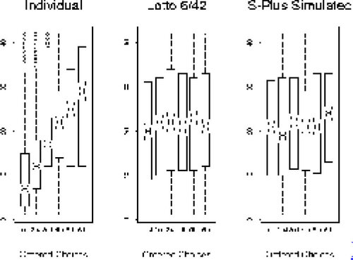
9 Individuals were asked to generate (and write down) their selections in any order. The intention was that this be interpreted to mean the order itself should be random (and we felt this was the implication), although one might interpret this as meaning “in any order you choose.” It is important that instructions to students not be ambiguous in this respect. In any case, it is clear that our Individual data show the tendency of people to generate numbers in increasing order. This is demonstrated nicely by the use of three sets of simultaneous ‘notched’ box plots in Figure 1. For the Individual data, we have notched box plots for the six selections in the order they were generated (written down), and similarly for the Lotto 6/42 and S-Plus Simulation sets. Non-overlapping notches from two such box plots indicate a significant difference in means at approximately the 5% level. Hence, the first, second, third, and fourth selections for the Individual data display a significant increasing trend. However, the only significant difference when considering the other two datasets is between the second and sixth selections in the S-Plus simulated data. Here we have an opportunity to show students how careful one must be in making multiple comparisons. In looking for significant differences among ordered selections in any one of the three sets of data, we are actually making $\left(\frac{6}{2}\right)$ = 15 comparisons. Hence, if the order in a selection is truly random (as it should be in each of the datasets Lotto 6/42 and S-PLUS Simulation), we would expect about$\frac{1}{20}$(15+15) =1.50 significant differences at the 5% level to appear by chance alone (and we observed 1!).

Figure 1. Box Plots of Ordered Selections of Six Numbers from {1, 2, 3, …, 42}.

10 In collecting the Individual data, students were, of course, asked to ‘randomly’ generate numbers, in contrast to picking their favorite or lucky numbers. Truly random methods of generating six-tuples should, of course, yield uniform marginal distributions. In m truly random selections of n-tuples for Lotto n/N, we would expect each number {1, 2, 3, …, N} to be chosen approximately $m\cdot \frac{n}{N}$ times (and hence for Lotto 6/42 approximately $\frac{m}{7}$ times). Figure 2 presents histograms for the frequencies with which each of the numbers {1, 2, 3, …, 42} were selected in our three datasets. Horizontal lines are drawn in each case at m/7 (234/7 = 33.4 for the Individual data and 264/7 = 37.7 for the Lotto 6/42 and S-Plus Simulation datasets). One could also use histograms with percentages instead of absolute frequencies, and for Lotto 6/42 one would expect each number to appear in about 14.3% (or 1/7) of the selections.

Figure 2. Frequency of Numbers When Selecting Six From {1, 2, 3, …, 42}. The horizontal lines in each case represent the expected number under complete randomness.

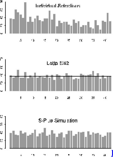
11 Note that in spite of the request for individuals to chose ‘randomly,’ the histogram for the Individual data clearly shows a slight tendency for individuals to pick smaller numbers. If one considers, for example, the lower and upper halves of the possible numbers [1-21] and [22-42], respectively, then 15 of the first half were selected more often than would be expected, while only two of the second half (27 and 41) were likewise selected. In contrast to this, the histograms for the Lotto 6/42 and S-Plus Simulation datasets seem to display no unusual features of this nature. Although students do not find these observations very surprising, results like these can lead to interesting discussions as to why smaller numbers in general (and some specific ones in particular) might be favored. Before showing students histograms of this type it might be useful to ascertain what they think they will look like!

12 It is natural to ask if there is any ‘significance’ in these histograms, and, in particular, whether the selected numbers are uniformly distributed on {1, 2, 3, …, 42}. One naturally thinks of using a x² goodness of fit test, but one must be careful to remember that the selections are samples of size n taken without replacement, and hence the numbers in a selection are not completely independent. In “Tests of Uniformity for Sets of Lotto Numbers,” Joe (1993) derives tests for the uniformity of marginals for the distributions of single numbers, pairs, and triples such as those arising in Lotto n/N (although a x² test for equiprobability of Lotto numbers first appeared in Morgenstern (1979) and later in Henze (1982)). In particular, he shows that the asymptotic distribution (under the hypothesis of truly random generation) of $$x^2=\frac{N-1}{N-n}{\displaystyle \sum \frac{{(0_i-E)}^2}{E}}$$(1)

is x² with N-1 degrees of freedom (where $E=m\frac{n}{N}$ and m is the number of selections). For Lotto 6/42, the test statistic takes the form $$x^2=\frac{41}{36}{\displaystyle \sum _1^{42}\frac{{(0_i-m/7)}^2}{m/7}}$$(2)

13 Our observations give the results in Table 1. Noting that x²_41,.99 = 64.95 and x²_41,.95= 56.94, we clearly may reject the hypothesis of uniform univariate marginals for the data collected from our students, while the test statistics for the Lotto 6/42 and S-Plus Simulation datasets are very much in line with what one might expect from truly random generators. Although the histograms presented in Figure 2 give a clear indication of the bias that individuals have in trying to select random numbers, students are normally quite impressed by the dramatic difference between the value of the Individual x² test statistic and the values of the other two test statistics.

Table 1. Testing for Uniform Univariate Marginals

Dataset	m	x^2
Individual	234	261.05
Lotto 6/42	264	39.64
S-Plus Simulation	264	37.82

3. Means of Selections in Lotto

14 The study of sample means and variances of observations can also give one insight into the randomness of the selections. If $x=(x_1,x_2,\mathrm{\dots },x_n)$ represents n numbers (in the order selected) from {1, 2, …, N}, we let $\overline{x}$ and s2 be the sample mean and sample variance, respectively. From the basics of survey sampling, we know that if the selections are truly random, then $$E(\overline{x})=\frac{N+1}{2}andV(\overline{x})=\left(\frac{N-n}{N-1}\right)\left(\frac{{\sigma }^2}{n}\right)=\frac{(N+1)(N-n)}{12n}.$$(3)

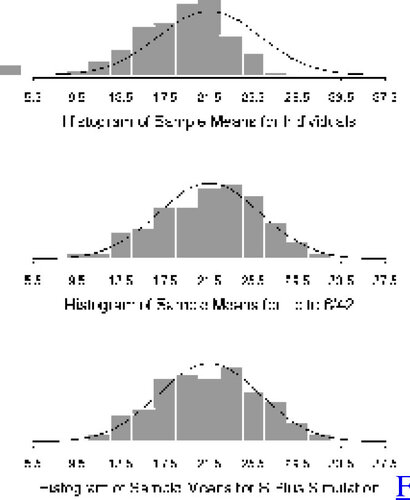
15 For Lotto 6/42, we have coincidentally that $E(\overline{x})=V(\overline{x})=\mathrm{21.5.}$ Hence for random selections of 6 from 42 (as in Lotto 6/42), we would expect $\overline{x}$ to be approximately normally distributed, and in particular that $\overline{x}$~N(21.5, 21.5). In Figure 3, we see histograms of the sample means $\overline{x}$ for each of our three datasets. Although the histogram for the means from the Individual data is slightly skewed to the left with a few very small values, the three histograms are roughly normal in shape (note that means for the Individual data seem to be centered slightly to the left of 21.5). Students should, however, be aware of the impact of interval width on the shape of a histogram, and that QQ plots (and, in this case, normal quantile plots) are more robust and usually more informative in comparing distributions. These datasets offer a good opportunity to demonstrate this to students.

Figure 3. Histograms of Sample Means.

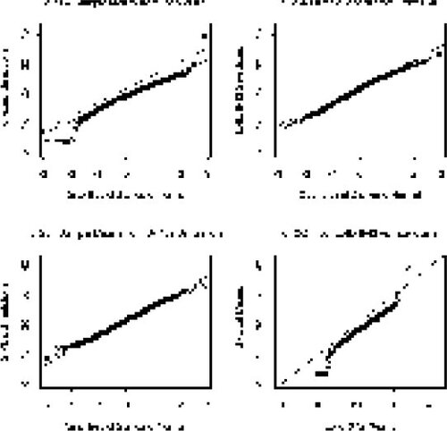
16 In Figure 4, we have normal quantile plots of the means for the three datasets, together with a QQ plot of the means for the Lotto 6/42 and Individual data (Figure 4d). For the normal quantile plots, the dotted line $y=21.5+\sqrt{21.5x}$ represents where the means should fall for N(21.5, 21.5) data, and the solid line is the line connecting the quartiles (this is used in preference to a least squares line as it is more robust to outliers). The normal quantile plot for the Individual means $\overline{x}$ in Figure 4a suggests a distribution somewhat similar in shape to a normal distribution (due to the linearity of the vast bulk of observations) but which is centered to the left of 21.5 and which has slightly heavier tails (particularly the left) than a normal distribution. There are a few “individual” selections that should clearly be termed “outliers.” Five people selected the numbers (1, 2, 3, 4, 5, 6) in that order, while one individual selected (42, 41, 40, 39, 38, 37). One should certainly question whether or not the students making these selections were really trying to be random! These “outliers,” however, do not have a significant impact on our inferences about the mean ${\mu }_{\overline{x}}$ of $\overline{x}$ for individual selections. For example, in testing H₀:${\mu }_{\overline{x}}$= 21.5 on the basis of our Individual dataset, we observe a t statistic of -8.56, while a 95% confidence interval for ${\mu }_{\overline{x}}$ is [18.16, 19.40], indicating a bias on the order of -2.72. In particular, we would be confident that when asked to perform as random generators for Lotto 6/42, our students tend (on the average) to select numbers at least 2 smaller than a truly random generator. Figures 4b and 4c lend good support for the N(21.5, 21.5) distribution of $\overline{x}$ for the Lotto 6/42 and S-Plus Simulation datasets. Figure 4d indicates a clear shift (towards smaller values) for the distribution of $\overline{x}$ for Individuals when compared with the Lotto 6/42 data.

Figure 4. Normal Quantile and Quantile/Quantile Plots for the Means. For the normal quantile plots, the dotted lines represent where the data should fall under complete randomness, while the solid lines connect the quartiles.

4. Variability in Selections of Numbers

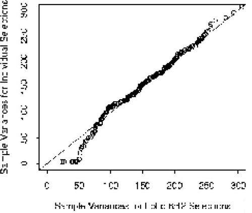
17 The observations or selections $(x_1,x_2,\mathrm{\dots },x_n)$ are multivariate, and we might naturally ask about what type of spread one would expect in a selection that is randomly generated. The sample variance s2 of a selection is a natural measure of spread to consider. In general for Lotto n/N, one may easily verify that E(s2) = N(N + 1)/12, which for Lotto 6/42 gives E(s2) = 150.5. In Figure 5, we see a QQ plot of the sample variances from the Individual selections, in comparison with those from Lotto 6/42. The distribution of s2 from the Individual selections compares reasonably well with that from Lotto 6/42, except in the tails (particularly the left tail). The Individual selections seem to be more skewed to the left (in this case because a small number of people made very concentrated selections which resulted in very small values of s2).

Figure 5. QQ Plot of Sample Variances for Lotto 6/42 and Individual Selections.

18 There are, of course, many possible measures of variability or spread in a selection, and another somewhat natural one is what we will call the minimum gap (MG). We define the random variable MG as follows: $$MG(x_1,x_2,\mathrm{\dots },x_n)=\min \{x_{(i+1)}-x_{(i)}:i=1,\mathrm{\dots },n-1\}$$(4)

where (x₍₁₎,x₍₂₎,…, x_(n)) are the observations reordered in increasing order. Note that MG = 1 if and only if the selection contains two consecutive numbers. It is reasonably straightforward to derive the distribution of MG for random selections of n numbers from {1, 2, …, N} and to show that $$P(MG=l)=\frac{\left(\frac{N-(l-1)(n-1)}{n}\right)-\left(\frac{N-l(n-1)}{n}\right)}{\left(\frac{N}{n}\right)}forl=1,\mathrm{\dots },\left[\frac{N-n}{n-1}\right].$$(5)

See Haigh (1995), Kennedy and Cooper (1991), and Speckman (1991) for the derivation of this result and Henze

(1995, 1997) for further extensions.

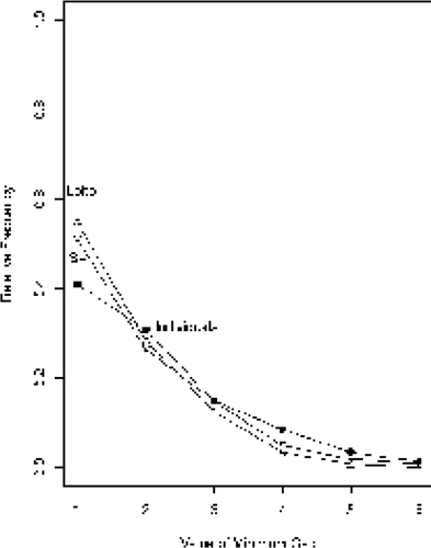
19 For Lotto 6/42, P(MG = 1) = 0.56 is the probability of a selection containing two consecutive numbers. Students usually find it very surprising and nonintuitive that it is more likely than not that a random selection will contain two consecutive numbers. Before giving students the probability of two consecutive numbers appearing in Lotto, it is a worthwhile exercise to test their intuition by asking them for estimates of it! In Figure

6, we have relative frequency polygons for the minimum gap MG for our three datasets. We see that Individuals have a clear tendency to spread out their selections more than one would expect from truly random selections, and in particular, the observed number of minimum gaps equal to one is unexpectedly low.

Figure 6. Frequency Polygons for the Minimum Gap.

20 A summary of the distributions of the random variable MG for the three datasets is given in Table 2 together with the corresponding x² goodness of fit statistics. These results clearly indicate that individuals are reluctant

to make selections containing consecutive numbers.

Table 2. Observed (O) and Expected (E) Values and x² Goodness of Fit Statistics for the Minimum Gap

Data	Individual	Lotto 6/42	S-Plus Simulation
m	234	264	264
MG	O (E)	O (E)	O (E)
1	96 (130.3)	145 (147.0)	135 (147.0)
2	72 (63.3)	75 (71.4)	70 (71.4)
3	35 (27.2)	33 (30.7)	39 (30.7)
≥ 4	31 (13.2)	11 (14.9	20 (14.9)
x^2	36.45	1.40	5.00

5. Conclusions

21 The whole concept of randomness is a delicate one, and one about which considerable research has been done, particularly in the field of psychology. Reichenbach (1949) claimed that humans are unable to produce a random sequence of responses, even when explicitly asked to do so, and considerable research since then (including our work) generally supports this. Many teachers/lecturers have told us of classroom activities they use to get students thinking about randomness, and Green (1997) gives an interesting account of an experiment on recognizing randomness.

22 How well can individuals perform when they attempt to be random generators for a game like Lotto? Some interesting insights into human intuition about randomness may be obtained by asking a class of students to participate in an exercise that tries to answer this question. We asked each of the students in a large class to act once as a random generator for the winning numbers in our Irish National Lottery - Lotto 6/42 game. The results were then analysed and compared with actual recent winning selections in our Lotto game, as well as with another set simulated by computer. Using boxplots, histograms, QQ-plots, and some basic measures of spread in a sample, one is able to generate interesting classroom discussions about biases that individuals seem to possess. We observed (perhaps not surprisingly) that there seems to be a propensity for individuals to select numbers in increasing order. We also observed that individuals tend to select numbers which on the average are smaller (by at least two) than would be expected from a truly random generator. Of course, in other countries or states where a different form of Lotto is played, the results will probably differ. When it comes to the spread in a selection, we observed that individuals tend to make selections that are reasonably spread out as measured by sample variance, but not in other ways (for example, as measured by the so-called minimum gap in a selection). In particular, we observed a clear reluctance of individuals (compared to a truly random generator) to make selections containing consecutive numbers.

References

- Green, D. (1997), “Recognizing Randomness,” Teaching Statistics, 19(2), 36–38.
- Haigh, N. (1995), “Inferring Gambler’s Choice of Combinations in the National Lottery,” Bulletin of the Institute of Mathematics and its Applications, 31(9-10), 132–136.
- Henze, N. (1982), “Verhalten des Chi-Quadrat-Tests fur Prufung der Gleichwahrscheinkeit der Lotto-Zahlen bei Nichtgultigkeit der Hypothese,” Metrika, 29(2), 135–139.
- Henze, N.– (1995), “The Distribution of Spaces on Lottery Tickets,” Fibonnaci Quarterly, 33(5), 426–431.
- Henze, N.–– (1997), “A Statistical and Probabilistic Analysis of Popular Lottery Tickets,” Statistica Neerlandica, 51(2), 155-163.
- Joe, H. (1993), “Tests of Uniformity for Sets of Lotto Numbers,” Statistics and Probability Letters, 16, 181–188.
- Kadell, D., and Muisaker, D. (1991), “Lotto Play: The Good, the Fair and the Truly Awful,” Chance, 4(3), 22–25.
- Kennedy, R. E., and Cooper, C. N. (1991), “The Statistics of the Smallest Space on a Lottery Ticket,” Fibonacci Quarterly, 29(4), 367–370.
- Morgenstern, D. (1979), “Der chi-Quadrat-Test for Prufung der Gleichwahrscheinlichkeit der Lotto-Zahlen,” Mathematisch-Physikalische Semesterberichte, 26(1), 36–39.
- Reichenbach, H. (1949), The Theory of Probability, Berkeley: University of California Press.
- Speckman, P. (1991), “Lottery Loophole Explained,” Stats, 5, 16.
- Ziemba, W. T. (1986), Dr. Z’s 6/49 Lotto Guidebook, Vancouver and Los Angeles: Dr. Z Investments, Inc.