A Model of Classroom Research in Action: Developing Simulation Activities to Improve Students' Statistical Reasoning

Abstract

Researchers and educators have found that statistical ideas are often misunderstood by students and professionals. In order to develop better statistical reasoning, students need to first construct a deeper understanding of fundamental concepts. The Sampling Distributions program and ancillary instructional materials were developed to guide student exploration and discovery. The program allows students to specify and change the shape of a population, choose different sample sizes, and simulate sampling distributions by randomly drawing large numbers of samples. The program provides graphical, visual feedback that allows students to construct their own understanding of sampling distribution behavior. To capture changes in students' conceptual understanding we developed diagnostic, graphics-based test items that were administered before and after students used the program. An activity that asked students to test their predictions and confront their misconceptions was found to be more effective than one based on guided discovery. Our findings demonstrate that while software can provide the means for a rich classroom experience, computer simulations alone do not guarantee conceptual change.

Keywords:

• Assessment
• Computer microworlds
• Conceptual change
• Diagnostic testing
• Sampling distributions
• Statistical instruction

1. Introduction

1 This paper presents an example of classroom research in the context of an introductory statistics course. “Classroom research,” also referred to as “action research,” is a promising model of educational research, where the main goal is to gain insight into problems, their definitions, and their sources (Hollins 1999, Hopkins 1993, Noffke and Stevenson 1995). In contrast to more traditional forms of research, classroom research does not attempt to answer questions definitively nor to find solutions to problems. While classroom research is often described in the context of elementary and secondary education, it is currently being recommended for post secondary instructors as a tool for studying and improving their classes (Cross and Steadman 1996). Building on previous models as well as our own experiences, we developed a model of classroom research for statistics education. The basic questions that structure our model are outlined below in four stages:

1.	What is the problem? What is not working in the class? What difficulties are students having learning a particular topic or learning from a particular type of instructional activity? The identification of the problem emerges from experience in the classroom, as the teacher observes students, reviews student work, and reflects on this information. As a clearer understanding of the problem emerges, the teacher may also refer to published research to better understand the problem, to see what has already been learned and what is suggested regarding this situation, and to understand what might be causing the difficulty.
2.	What technique can be used to address the learning problem? A new instructional technique may be designed and implemented in class, a modification may be made to an existing technique, or alternative materials may be used, to help eliminate the learning problem.
3.	What type of evidence can be gathered to show whether the implementation is effective? How will the teacher know if the new technique or materials are successful? What type of assessment data will be gathered? How will it be used and evaluated?
4.	What should be done next, based on what was learned? Once a change has been made, and data have been gathered and used to evaluate the impact of the change, the situation is again appraised. Is there still a problem? Is there a need for further change? How might the technique or materials be further modified to improve student learning? How should new data be gathered and evaluated?

These questions outline a basic plan that statistics instructors may use to carry out a focused research project within their own classrooms. These stages are carried out in an iterative rather than a linear manner, as the questions in stage 4 naturally lead back to those in stage 1.

2 The results of many classroom research studies may not be viewed as suitable for dissemination, as they often focus on a particular class setting and are not generalizable. Many also include anecdotal information about the implementation and the assessment information gathered. However, we argue that ongoing classroom research projects such as the one described in this paper, when done carefully and in collaboration, often yield valuable insights into the teaching and learning of statistics that are of benefit to the education community.

3 Our project stemmed from concern about the difficulty many students have in understanding concepts underlying statistical inference, particularly with sampling distributions. We believed that simulation activities demonstrated on the computer could help students to better visualize and understand these concepts. However, after using what we considered excellent software, we found that students still demonstrated a lack of understanding as well as some troubling misconceptions about sampling distributions. The following sections describe how we used the four stages of the classroom research model listed above to implement a project that ultimately improved many students’ understanding of important concepts that are foundational to an understanding of inference.

4 For our first step, we focused on the faulty reasoning students exhibit with sampling distributions of sample means. Secondly, we utilized software simulations to allow students to explore and interact with sampling distributions. Thirdly, we developed a pretest and posttest to determine the impact of the activity on students’ reasoning. Reflecting on the data gathered and our observations of students using the software, we continued the cycle of revising the software, an instructional activity for using the software, and the assessment instruments.

2. What Is the Problem?

5 We perceived that many of our students develop a shallow and isolated understanding of important foundational concepts related to statistical inference, in particular, ideas of sample, population, distribution, sampling, and sampling variability. We were concerned that many students who pass a statistics course do not develop the deep understanding needed to integrate these concepts and apply them in their reasoning. As teachers who have taught introductory statistics courses for several years, we were particularly disappointed by our students’ continual inability to explain or apply their understanding of sampling distributions. We found this

lack of understanding particularly troublesome as we see the concept of sampling distributions as crucial to the understanding of statistical inference. We began to develop our own methods for teaching sampling distributions that would facilitate integration of these ideas and enhance understanding of the basic processes involved. These methods combined hands-on activities in class with use of interactive simulation software. However, students were still demonstrating a clear lack of understanding and an inability to apply their knowledge when solving statistical problems.

6 We decided to investigate the published literature to see if others have struggled with this problem and to see what we might learn from this body of literature. We found several existing simulation packages that have been used to teach sampling distributions (e.g., Behrens 1997, Cumming and Thomason 1998, Finch and Cumming 1998 , Velleman 1998). However, all appear to be used to illustrate the sampling process and creation of a sampling distribution in similar ways. They are typically used either as a demonstration offered by the instructor during a class or as a lab activity that students experience individually or working in pairs. These implementations require students to focus on what happens when different populations are used and with different sample sizes. This makes sense as a logical way to use the software. Indeed, it is the way we first conceptualized and used our own simulation software.

7 We also found that despite the accepted approach used to integrate simulation software into a statistics class, there is little published research describing and evaluating such an approach. While the motivation for these programs is to provide improved instructional experiences, most of the authors describe the nature of the program and demonstrate how it can be used in the classroom, but they do not report any evidence that the program improves learning or understanding of sampling distributions (e.g., Behrens 1997, Davenport 1992, Schwarz and Sutherland 1997). Several authors have commented on the perceived benefits of using simulations in the introductory statistics course. Simon (1994, Simon and Bruce 1991) claims that simulations based on resampling methods allow students to deal with statistical problems that even trained, experienced statisticians find difficult and help students gain insights into the mechanisms that produce phenomena such as sampling distributions by making the process observable. Glencross (1988) describes how simulations can provide (theoretically) ideal conditions for the learning of an abstract concept like sampling distributions by providing multiple examples of the concept and allowing students to experiment with all of the variables that form the concept. While both of these authors report anecdotally that students are more engaged and interested in learning about statistics when simulations are used, neither provides assessment information to demonstrate that simulations actually produce additional or deeper conceptual understanding.

8 In the few cases where assessment has been conducted, the results have not been impressive. Hodgson (1996) based his assessment on open-ended items completed by ten students in a summer graduate course designed to provide the foundations for teaching statistics at the precollege level. While modest improvements were found in students’ understanding of sampling distributions, student conceptions were only partially correct. Furthermore, students appeared to have developed incorrect assumptions about the nature of sampling distributions as a result of their experience with the computer simulation. Additionally, Schwartz, Goldman, Vye, and Barron (1997) reported only modest changes (about a 15% improvement) from pretest to posttest for sixth grade students when anchored instruction and computer simulations were combined to teach about sampling distributions. These findings echo a point made by Nickerson (1995) that a computer microworld in and of itself does not guarantee the development of correct understanding (see also Behrens 1997 and the Cognition and Technology Group at Vanderbilt 1993).

3. What Technique Can Be Used to Address the Learning Problem?

9 Several years ago, one of us (delMas) decided to develop software for the Macintosh computer to illustrate the creation of sampling distributions. While delMas has served as the software’s programmer, the other two authors have been instrumental in its development through their use of the program in their respective educational settings. Development of the program has also benefited from our knowledge of the research literature on educational technology. For example, Nickerson (1995) offers some maxims for fostering understanding that point to the need for simulations:

1.	View learning as a constructive process where the task is to provide guidance that facilitates exploration and discovery.
2.	Use simulations to draw students’ attention to aspects of a situation or problem that can easily be dismissed or not observed under normal conditions.
3.	Provide a supportive environment that is rich in resources, aids exploration, creates an atmosphere in which ideas can be expressed freely, and provides encouragement when students make an effort to understand.

10 Nickerson points out that while technology does not promote understanding in and of itself, it does represent a tool that can readily incorporate the principles listed above. Real-world models can be developed as explorable microworlds that allow students to test assumptions, make predictions, highlight misconceptions, and promote active processing by changing parameters and defining entities. Computer simulations can present dynamic representations that go beyond the modeling of static entities by making the processes that produce phenomena more concrete and observable.

11 Snir, Smith, and Grosslight (1995) provide some additional recommendations. They suggest that a simulation is conceptually enhanced when it allows students to perceive phenomena that cannot be directly observed under normal conditions (e.g., theoretical and abstract concepts), provides explicit representations for sets of interrelated concepts, and promotes mapping between different representations of the same phenomena. These authors recommend that instructional materials and activities be designed around computer simulations that emphasize the interplay among verbal, pictorial, and conceptual representations. Snir, Smith and Grosslight have observed that most students will not explore multiple representations on their own accord and require prompting and guidance.

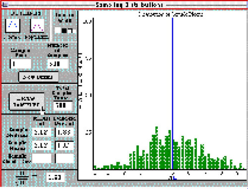
12 These ideas and characteristics are present in both the software and the activity we initially developed to guide students’ use of the software. We focus here on use of the software to explore the behavior of sample means. The Sampling Distributions program (see Figure 1) and instructional materials were developed to facilitate guided exploration and discovery by allowing students to change the shape of a theoretical population or the size of the samples drawn, and then to run a simulation by drawing a large number of random samples. In the Population window a student can create a predefined distribution shape by clicking on one of the preset buttons, or can use the up and down arrows below the graph to “push” the distribution into any shape they wish. The student can then switch to the Sampling Distributions window (see Figure 2) to draw random samples of a specified sample size from the population.

Figure 1. Creating a Normal Distribution for the Population.

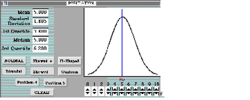
Figure 2. Drawing Random Samples to Create a Sampling Distribution.

13 The program has evolved significantly over the first few years of its use. The initial program allowed students to select several common forms for the population distribution (normal, skewed right, skewed left). The program graphed the sampling distributions for the mean and median, and provided summary statistics for these distributions (median, mean, average sample standard deviation, and standard error). From our experience using the program in our classrooms and from students’ comments, we found that students could become overwhelmed with the amount of information they were receiving. Changes were made to the program to highlight the most important concepts we wanted them to focus on. An early change to the program involved clarification of the summary statistics. For example, the program now provides the standard deviation of the sample means, as well as the value of for comparison. The sample statistics of the sampling distribution are now also presented in a tabular format that clarifies the distinction between sample statistics and statistics of the sample statistics.

14 To help students see the long run patterns in the sampling distributions, we added an option that allows them to “add more” samples to an existing distribution. This allows students to build up a sampling distribution one sample at a time, 10 samples at a time, or in any increment they choose. To further enhance students’ ability to identify and contrast common patterns, two “template” buttons were added. These buttons superimpose the shape of either the population or of the normal distribution predicted by the Central Limit Theorem on top of the sampling distribution. The templates can be used by the students to help judge whether the sampling distribution is following either of these shapes. Students can also expand or contract the horizontal scaling to more easily see the shape of the sampling distribution. Many of these changes arose from consideration of students’ comments after they used the program.

15 In the initial form of the instructional activity, students were instructed to create a normal distribution in the Population window (see Figure 1). They were then instructed to switch to the Sampling Distributions window (see Figure 2) where they changed the sample size in increments from n = 5 to n = 100, each time drawing 500 random samples. The students recorded the sampling distribution statistics that resulted for each sample size, described the shape, spread, and center of the sampling distributions, and related these observations to the parameters and shape of the population. After completing the last run for n = 100, several questions were presented to the students to help them understand the effects of sample size on shape, center, and spread of sampling distributions: What is the relationship between sample size and the spread of the sampling distributions? At what sample sizes do each of the sampling distribution statistics begin to stabilize (not change significantly as the sample size is increased)? Did the sampling distribution statistics provide good, accurate estimates of the population parameters? Overall, did the sampling distribution statistics behave in accordance with the Central Limit Theorem? After running simulations for a population with a normal distribution, students were instructed to repeat the activity for a skewed population and for a population with “an unusual shape.” The activity and questions were intended to direct student attention toward the different pieces of information that are related to the Central Limit Theorem and to prompt them to test out their assumptions about the behavior of sampling distributions.

4. What Type of Evidence Can Be Gathered to Show Whether the Implementation Is Effective?

4.1 Assessment Instruments

16 To assess the effects of the program and activity on students’ conceptual understanding of sampling distributions, we felt that it was necessary to go beyond traditional questions that asked students to state the expected mean for a sampling distribution, calculate the standard error of the sample mean, or state how the standard error changes with changes in sample size. While these are important and relevant questions, we first wanted to see if students could demonstrate a visual understanding of the Central Limit Theorem’s implications for sampling distributions. Therefore, we set about the task of designing graphics-based measurement items.

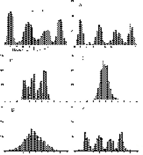
17 Two of the authors had already developed graphics-based items for testing students’ understanding of statistical power (Garfield and delMas 1994). Using some of the ideas from this earlier work, a set of problem situations was developed. In an early version, test items were based on four population distributions that represented a normal distribution, a positively skewed distribution, a symmetric bimodal distribution, and an irregular distribution with four peaks, each peak being of a different height. In a later version we decided to add one more irregularly shaped population as a fifth item in order to get a better understanding of students’ responses when they encounter atypical situations. The five population distributions are illustrated in Figure 3. Each problem situation consisted of a graph that depicted the population distribution and five additional graphs that represented possible distributions of sample means for samples drawn at random from that particular population (see Figure 4 for an example; Appendix A shows all five problems).

18 Each problem consisted of two parts. Part A asked the student to select the graph that represented a distribution of sample means for 500 random samples, each of a relatively small sample size (n = 1 or n = 4). Part B asked students a similar question, but the sample size was larger (n = 9, n = 16, or n = 25). For both parts of the question, students were encouraged to write the reasons for their choices. The five histograms of possible sampling distributions were designed so students could display several types of reasoning (correct and erroneous).

Figure 3. Population Distributions Used for the Assessment Items.

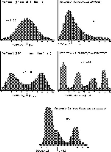
Figure 4. Problem 4 Population Distribution and Possible Distributions of Sample Means.

4.2 The Classroom Settings

19 The research reported in this paper was conducted in collaboration among the three authors at their respective institutions and, therefore, represents three different classroom settings. While these three settings do not represent every possible configuration of the college introductory statistics course, we believe that they provide enough diversity to allow some generalization to other settings. Across the three settings, students vary with respect to their pre-college experiences. The courses vary in the way material is presented, topics are emphasized, and activities are structured. Therefore, we believe that instructional approaches found to be effective across these three settings may also be effective across many of the diverse settings in which introductory statistics is taught.

20 The first setting was in an introductory statistics course offered through the Mathematics Department at University of the Pacific, a private university in northern California. Most of these students take the statistics course to fulfill a General Education requirement. The course enrolled a range of students from freshmen to seniors with numerous majors such as business, sciences, liberal arts, and engineering. Students worked on lab activities each week during a one-hour lab session. The lab sections were limited to 25 students so each student could work at a computer. Students were encouraged to work in pairs, and were required to submit a written report of a lab activity within one week of each lab session.

21 The second setting was in an introductory statistics course offered through the College of Education at the University of Minnesota. Most students enrolled in this course to fulfill a mathematical reasoning requirement for their liberal arts degrees. The majority of students were juniors and seniors majoring in the arts, social sciences, or humanities. The course was taught using an active learning format. Students read textbook chapters before coming to class and spent class sessions gathering and analyzing data and performing experiments. Two class sessions were held in a computer classroom each term where students were introduced to a statistical computing package and statistical resources on the internet.

22 The third setting was in an introductory statistics course offered through the General College, a developmental education college at the University of Minnesota. The General College is an open admissions college that enrolls nontraditional, under-served, under-prepared students who would not normally be admitted to the University. The statistics course, however, was taken by a wide range of students at the University of Minnesota to fulfill the University’s mathematical reasoning requirement. The enrollment was limited to 30 and the course taught in a lab equipped with one computer per student. The class met for five hours each week during which time students completed one to three lab activities that typically involved the use of statistical software or computer simulations. Students often worked in pairs or groups.

23 In all three settings, students were expected to have read the appropriate textbook chapter on sampling distributions and the Central Limit Theorem prior to the activity. Students also engaged in a hands-on simulation of the Central Limit Theorem during a class period prior to using the Sampling Distributions program, although the same activity was not used at all three sites. The hands-on simulations consisted of students drawing random samples of specified sample sizes from a population of measurements (e.g., first term grade point averages of freshmen with sample sizes of n = 5, n = 10, and n = 25; dates of pennies with sample sizes of n = 1 and n = 4). Sample means were then calculated and graphed to create distributions of sample means for the different sample sizes. Class discussions involved comparison of the shape, center, and variability among the different distributions, as well as comparisons of the distribution statistics to values predicted by the Central Limit Theorem.

24 Students typically took between one and one-and-a-half hours to complete the sampling distributions activity using the software. Students worked in labs where each student had access to the program on an individual computer. While students worked at individual computers, they were encouraged to interact with each other and to compare results and conclusions.

4.3 Assessment Data

25 The test was first piloted in fall 1996 to two groups of students, 29 students at the private university and 20 students at the developmental education college. From student responses and histogram choices we were able to identify several different types of reasoning. In the first type, “correct reasoning,” students chose the correct pair of histograms for a problem. In the second type, “good reasoning,” students made reasonable choices that indicated minor errors in their thinking.

26 In general, good reasoning occurred when a student chose a histogram for the larger sample size that was shaped like a normal distribution and that had less variability than the histogram chosen for the smaller sample size. Perhaps the histogram chosen for the smaller sample size was incorrect, but the variability in the distribution was consistent with the stated sample size. For example, in Problem 1 (see Appendix A), the smaller sample size was n = 1. The graph selected for Part A might look like the population in shape and spread, but contain more than 500 sample means (e.g., graph D). Combining this choice with a graph E for the larger sample size would be considered “good reasoning.” As another example, for Problem 4 (see Figure 4), with a smaller sample size of n = 4, a student might select a histogram with less variability than the population and with a shape similar to that of the population (graph E) and then select graphs C or D for the larger sample size. These students were judged to display good reasoning, although they did not appear to understand that the curve of the sampling distribution can start to resemble a normal distribution even with a sample size of 4.

27 A third type, “larger to smaller reasoning,” was similar to good reasoning in that students chose a histogram with less variability for the larger sample size. These responses were not counted as good reasoning because either the variability in the histogram chosen for the smaller sample size was similar to the variability of the population when n > 1 (e.g., graph A in Problem 4 for n = 4), or both histograms had the shape of the population (e.g., graph E for n = 4 and graph B for n = 25 in Problem 4). A fourth type, “smaller to larger reasoning,” was designated for students who chose a histogram with larger variability for the larger sample size. Comments by some of these latter students indicated that they expected the sampling distribution to look more like the population as the sample size increased. Appendix B shows how different choices of graph pairs were categorized into these four reasoning categories for Problem 4. While these four categories covered about 80% to 90% of the responses for each problem, there were also a variety of other, less frequent, responses (e.g., choosing the same histogram for both sample sizes).

28 The students’ choices, written reasons, comments, and our own observations at the two sites were used to modify the test items. A framework was created so that the histogram choices were more consistent across the different problems. The framework was based on the four reasoning categories described above and is presented below in Table 1. The horizontal dimension of Table 1 represents the shape of the histogram for a possible sampling distribution, whereas the vertical dimension indicates the relative variability in the histogram. The test items were designed so that there was at least one histogram choice for each cell of Table 1, although some cells were represented by more than one histogram. The boldface letters in the cells of Table 1 refer to the sampling distributions given in Problem 4 (Figure 4) to illustrate how at least one example of each type was provided.

Table 1. Framework for Generating the Response Choices for Each Problem

	Normal Distribution	Population Distribution
Small Variability	C	B
Large Variability	D	A or E

NOTE: Histograms for Problem 4 are indicated by the bold face letters in each cell.

29 The framework of Table 1 guaranteed that each of the four reasoning types could be represented by students’ choices. For example, Problem 4 uses a sample size of n = 4 for Part A and a sample size of n = 25 for Part B. A correct choice of graphs would be a normal distribution with large variability for Part A and a normal distribution with small variability for Part B. Table 1 indicates that a correct pair of choices would be graphs D and C for the two respective parts of Problem 4. There are several ways to display larger to smaller reasoning, such as a choice of either graph A or E when n = 4 and graph B when n = 25. Examples of graph choices consistent with good reasoning were presented earlier.

30 Since students didn’t always produce self-generated explanations, and the explanations were sometimes hard to interpret, we also created a list that we felt captured students’ reasons for their choices. This allowed students to select the explanations that they were using, both ensuring a response and facilitating analysis. Based on the written responses students gave for the pilot test and on the framework in Table 1, we developed the following list of six statements that students could check to indicate their reasons for the histogram chosen in Part A (small sample size) of each problem (see Table 2). Students were given these same statements for Part B (larger sample size), with the addition of eight more statements that compared the histograms chosen in Part A and B (see Table 3). Students could select as many reasons as they felt were applicable.

Table 2. List of Reasons for Part A of Each Problem.

1.	I expect the sampling distribution to be shaped like a NORMAL DISTRIBUTION.
2.	I expect the sampling distribution to be shaped like the POPULATION.
3.	I expect the sampling distribution to have LESS VARIABILITY than the POPULATION.
4.	I expect the sampling distribution to have MORE VARIABILITY than the POPULATION.
5.	I expect the sampling distribution to have the SAME VARIABILITY as the POPULATION.
6.	I expect the bars of the sampling distribution and the population to have the SAME HEIGHT.

Table 3. List of Additional Reasons for Part B of Each Problem.

7.	I expect the second sampling distribution to have MORE VARIABILITY than the first.
8.	I expect the second sampling distribution to have LESS VARIABILITY than the first.
9.	I expect the second sampling distribution to look MORE like the POPULATION than the first.
10.	I expect the second sampling distribution to look LESS like the POPULATION than the first.
11.	I expect the second distribution to look MORE like a NORMAL population than the first.
12.	I expect the second distribution to look LESS like a NORMAL population than the first.
13.	I expect both sampling distributions to have about the SAME SHAPE.
14.	I expect both sampling distributions to have about the SAME VARIABILITY.

31 The new instrument was administered to 79 students who were registered in two different sections of introductory statistics at the private university and 22 students who took introductory statistics at the College of Education. Eighty-nine students who gave responses to all pretest and posttest items were used for the analyses. Detailed analysis of pretest and posttest results for one problem are presented in Appendix B which provides a discussion of patterns among students’ choices of sampling distributions and reasons. The results indicate that students’ choices of sampling distributions were very consistent with their indicated reasons.

32 Figure 5 presents a summary of results across the five problems for the pretest and posttest. Very few students chose the correct pair of graphs on the pretest (8%), and the average percent of correct choices remained quite low on the posttest (16%). Selection of the correct pair of graphs required estimation of the size of the standard error of sample means based on the sample size, which only a few students may think to perform.

Figure 5. Percent of Winter 1997 Students (N = 89) Who Indicated Acceptable Reasoning Under Three Different Criteria.

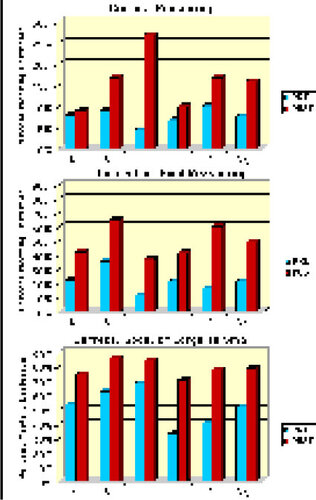
33 A second criterion of acceptable reasoning in which correct and good choices were combined provides another view of the pretest to posttest changes. On average, students displayed acceptable reasoning under this second criterion on only 22% of the items on the pretest, increasing to an average percent of about 49% on the posttest. While this is a considerable improvement, it indicates that students were not consistently applying their knowledge of sampling distributions across the five problems. Inspection of the averages for the “Correct or Good” criterion on the posttest indicates that the normal distribution (Problem 1), multi-modal distribution (Problem 3), and the irregular distribution of Problem 4 provided the most difficulty for students. The last criterion, which combines the reasoning types of correct, good, and larger to smaller variance, shows that most students had some grasp of how sample size affects a sampling distribution prior to using the program, and that most had at least gained an understanding that the variance of the sampling distribution decreases as the sample size increases by the posttest.

5. What Should Be Done Next, Based on What Was Learned?

34 We were surprised and disappointed to find that many of our students still displayed some serious misunderstanding of sampling distributions after working with the Sampling Distributions program. While there was a significant change from pretest to posttest, there was still a substantial number of students who did not appear to understand the basic implications of the Central Limit Theorem. We came to recognize that good software and clear directions that point students to important features will not ensure understanding. We went back to the research literature, looked beyond statistics education, and considered the implications of a theory of conceptual change that has been applied to learning science (Posner, Strike, Hewson, and Gertzog 1982). This model proposes that students who have misconceptions or misunderstandings need to experience an anomaly, or contradictory evidence, before they will change their current conceptions. Ross and Anderson (1982) suggest that effective discrediting experiences are those that both require subjects to act upon their beliefs and increase the dissonance between their expectations and observed outcomes.

35 While contradictory experience is necessary, it is not sufficient for conceptual change. Research indicates that people, in general, are resistant to change and are very likely to find ways to either assimilate information or discredit contradictory evidence, rather than restructure their thinking in order to accommodate the contradictions (Lord, Ross, and Lepper 1979; Jennings, Amabile, and Ross 1982; Ross and Anderson 1982). Modern information processing theories (e.g., Holland, Holyoak, Nisbett, and Thagard 1987) suggest that it may be necessary to direct attention toward the features of the discrediting experience in order for the contradictory evidence to be encoded. Left to their own devices, people will attend only to those features that are predicted by their current information structure.

36 Building on our experiences using the software and the conceptual change model of learning, we developed a revised approach to teaching sampling distributions. We believed that the software program incorporated all the needed features to promote conceptual change, so we focused our attention on the nature of the activity, looking for a way to better direct student attention and promote the testing of assumptions.

37 As we sought a way to have students make their own predictions and then test them out using the Sampling Distributions program, we finally came upon the idea that the assessment instruments themselves might provide just what was needed. The activity was modified so that instead of testing out general population shapes for a variety of sample sizes, the students would actually test out the situations encountered in the pretest and, therefore, evaluate their responses to the pretest items. Additional problems were designed for the posttest that paralleled the pretest items but did not use the same population distributions. The Sampling Distributions program was also modified by the addition of two preset population buttons that allowed students to produce the population distributions for the fourth and fifth pretest problems. This made it possible for students to produce the exact shape and parameters without needless trial and error using the up and down arrows.

38 In the new version of the activity, students created the population presented for a problem on the pretest, then drew 500 samples at each of the sample sizes stated in Parts A and B of the pretest problem. Students were asked to circle the letter of the graph that looked most like the sampling distribution produced by the program. They were also asked to answer the following three questions when looking at the sampling distribution for Part A:

1.	How does the shape of the graph you chose compare to the shape of the population?
2.	How does the shape of the graph you chose compare to the shape of a normal distribution?
3.	How does the spread of the graph you chose compare to the spread of the population?

In addition to these same three questions, students were asked to respond to the following two questions when looking at the sampling distribution for Part B:

4.	How does the shape of the graph you just chose for Problem B compare to the shape of the graph you chose above for Problem A?
5.	How does the spread of the graph you just chose for Problem B compare to the spread of the graph you chose above for Problem A?

The new activity placed more emphasis on comparisons of the shape and variability of the distributions than on the recording of parameters and statistics, and required students to make a direct comparison of their pretest “predictions” with the sampling distributions produced by the program.

6. Assessment of the New Activity

39 In the spring and fall of 1997, a total of 149 students used the Sampling Distributions microworld with the new activity. Thirty-two of the students were enrolled at the private university, 94 took an introductory statistics course through the developmental education college, and 13 took their course through the College of Education at the University of Minnesota. Of the 149 students, 141 gave responses to all items on the pretest and posttest.

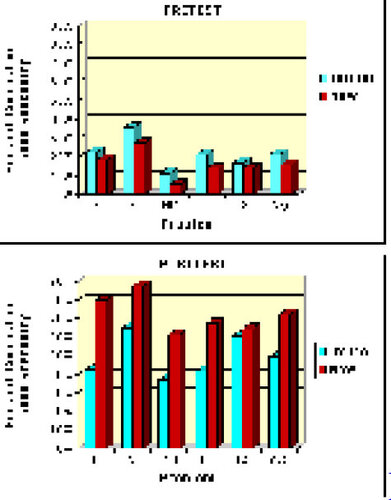
40 As can be seen in Figure 6, students who used the new activity had marginally lower percentages of acceptable reasoning on the pretest than the initial activity students. (See Figure 3 for the population distributions used in the five problems.) However, the percentages were higher on the posttest than the corresponding percentages for the initial activity students. On average, the new activity students went from having correct or good reasoning on 16% of the pretest items to having correct or good reasoning on 72% of the posttest items.

The most noticeable change, however, was in the average percentage of items on which students chose the correct pair of graphs. While the initial activity students chose the correct pair of graphs on an average of 16% of the posttest items, the new activity students were correct on 36% of the posttest items.

Figure 6. Comparisons of Student Reasoning Between the Initial (N = 89) and New Activity (N = 141) Using the “Correct or Good” Criterion.

41 Separate multivariate analyses of variance (MANOVA) were conducted for scores based on three different reasoning criteria: Correct choice only; Correct or Good choice; Correct, Good, or Larger to Smaller Choice. Each analysis consisted of two within and one between factors: item by test (pretest vs. posttest) by group (initial vs. new activity). Under all three criteria, posttest scores of students using the new activity were significantly higher than those who used the initial activity. Appendix C presents the details of the multivariate analyses of variance.

42 Our findings suggest that a straightforward presentation of the knowledge (for example, having students experience simulated sampling distributions from different types of populations, and for different size samples) doesn’t necessarily lead to a sound conceptual understanding of the core concepts. As a result, we’re excited about expanding our new instructional approach based on the model of conceptual change that has students make predictions and directly test them. We now strongly believe, as is supported in the research literature, that learning is enhanced by having students become aware of and confront their misconceptions. Students learn better when activities are structured to help students evaluate the difference between their own beliefs about chance events and actual empirical results (e.g., delMas and Bart 1989). We think the way to do this is with carefully guided experiences that use the types of computer microworlds we’ve been developing and exploring.

7. Future Directions: The Unfinished Story

43 Over the process of working together in different colleges and educational settings over a three-year period, we think we have learned much about how to better use simulation software with students to develop ideas of sampling and sampling distributions. As a continuation of the classroom research cycle, the authors met together for a few days to discuss the year’s research and to set goals for future research. We identified several new research questions aimed at examining how different aspects of the activity, software program, and student assessments affect students’ understanding of sampling distributions.

44 One idea is to investigate whether physical, hands-on simulations of sampling distributions conducted prior to the lab activity will facilitate students’ learning when they interact with the Sampling Distributions program. We also plan to develop and assess a new warm-up activity to help students understand how concepts developed during the first part of the course (such as measures of center, variability, distribution shapes, the normal curve) are represented in the Sampling Distributions program. This will allow different features of the software to be highlighted while at the same time helping students integrate their prior knowledge with visual representations created by the software program.

45 There are several variations of the activity that we want to investigate. One question is whether having the instructor give a demonstration of the software to the class or having the students learn the software on their own in a tutorial mode produce different outcomes. An extension of this idea is to compare a teacher-led activity where students work at the same pace to an individualized or group activity where students work at different paces. Another study will look at whether a debriefing discussion, where students compare their experiences and their understanding of sampling distributions, helps them to better understand the factors that affect sampling distributions.

46 We also plan to expand the assessment instruments. The pretest will include items that assess prerequisite knowledge in order to learn whether students’ understanding of prior concepts moderates their learning during the activity. The posttest will be expanded to include context-based problems that require students to apply the concepts and reasoning developed during the activity in order to look at transfer of learning. A delayed posttest is also planned that will consist of items similar to those on the posttest embedded into the final exam of the course. The posttest will help us assess whether the new additions to the activity enhance learning through additional integration and application of key ideas. The delayed posttest will allow us to determine the extent to which learning is retained or lost. The assessment instruments will also be used to investigate the effects of at least three different instructional approaches for comparison with our own: classes taught without the use of simulations, classes where simulations are based only on physical apparatus, and classes that use simulations produced by other software programs.

47 The research approach will be expanded by conducting student interviews. During individual taped interviews, students will be asked to describe what they are seeing and learning, as well as explain their understanding of concepts (such as variability) as they interact with the software program. We hope to gain a better understanding of students’ reasoning, what they are noticing, and how the activity impacts their learning.

48 In addition to expanding the activity and instruments to be used during the coming year, some changes will be made to the Sampling Distributions program. We plan to add a “slider” to the Sampling Distributions window (see Figure 2). The slider will be an L-shaped bar, representing the standardized value of an observation, that students can move along the horizontal axis, When the slider is positioned, the program will report the number and percent of sample means that fall below the z-value. The number and percent of sample means that are expected to fall below the z-value according to the standard normal distribution will also be displayed. Thus, the slider will provide another tool students can use to judge how well the sampling distribution is represented by a normal distribution. Comparing the number of observations below a particular value for different sample sizes will also provide students with a concrete measure of how the variability in sample means changes with sample size.

49 A second change will be the addition of a window that displays the distribution and statistics for each individual sample. Students will be able to scroll from one sample to the next. We hope that the inclusion of a Samples window will allow students to compare the distribution of the sample with the distribution of the sample means side-by-side. The activity will prompt students to note the different effects of sample size on the two types of distribution.

50 A third change will be the addition of a Standard Distributions window that allow students to compare the distributions of z-values and t-values generated by the samples. The distribution of t-values should follow Student’s t-distribution more closely than the standard normal distribution for small sample sizes, but become more like the standard normal distribution as sample size increases. Statistics such as the mean and standard deviation for each distribution of standardized values, as well as counts and percents expected by the standard normal distribution and Student’s t-distribution, will be displayed. We plan to research whether the new window helps students extend their concepts of sampling distributions to standardized values and whether it motivates their understanding of why the t-distribution is a better representation of the sampling distribution when the population variance is unknown.

51 We believe that collaborative, classroom research is an exciting and productive model for research in statistics education. We encourage other statistics faculty to try out this model in their own classrooms as a way to better understand and improve student learning of statistics. We also encourage faculty who would like to become part of our collaborative project to examine and try out our software, activities, and assessment instruments (http://www.gen.umn.edu/faculty_staff/delmas/stat_tools/index.htm). This website also presents teachers’ guides that describe prerequisite knowledge students need to complete an activity, common misconceptions that students display when reasoning about the statistical concepts presented in an activity, and the goals of an activity.

Acknowledgments

This research was supported by a Grant-In-Aid from the University of Minnesota and a National Science Foundation grant from the Division of Undergraduate Education (DUE-9752523). Materials produced under this grant can be obtained at http://www.gen.umn.edu/faculty_staff/delmas/stat_tools/index.htm . We also want to thank the reviewers of this paper whose comments helped to significantly shape and focus the content. An earlier version of this paper was presented at the 1997 Joint Statistical Meetings in August 1997 in Anaheim, CA.

References

- Behrens, J. T. (1997), “Toward a Theory and Practice of Using Interactive Graphics in Statistical Education,” in Research on the Role of Technology in Teaching and Learning Statistics: Proceedings of the 1996 International Association of Statistics Education (IASE) Roundtable, eds. J. B. Garfield and G. Burrill, Voorburg, The Netherlands: International Statistical Institute, pp. 111–122.
- Cognition and Technology Group at Vanderbilt (1993), “Anchored Instruction and Situated Cognition Revisited,” Educational Technology, 33, 52–70.
- Cross, K. P., and Steadman, M. H. (1996), Classroom Research: Implementing the Scholarship of Teaching, San Francisco: Jossey-Bass Publishers.
- Cumming, G., and Thomason, N. (1998), “Statplay: Multimedia for Statistical Understanding,” in Proceedings of the Fifth International Conference on Teaching Statistics, Nanyang Technological University, Singapore: International Statistical Institute., pp. 947–952.
- Davenport, E. C. (1992), “Creating Data To Explain Statistical Concepts: Seeing Is Believing,” in Proceedings of the Section on Statistical Education of the American Statistical Association, pp. 389 394.
- delMas, R., and Bart, W. M. (1989), “The Role of an Evaluation Exercise in the Resolution of Misconceptions of Probability, Focus on Learning Problems in Mathematics, 11(3), 39–54.
- Finch, S., and Cumming, G. (1998), “Assessing Conceptual Change in Learning Statistics,” in Proceedings of the Fifth International Conference on Teaching Statistics, Nanyang Technological University, Singapore: International Statistical Institute, pp. 897–904.
- Garfield, J., and delMas, R. (1994), “Students’ Informal and Formal Understanding of Statistical Power,” paper presented at the Fourth International Conference on Teaching Statistics (ICOTS4), Marrakech, Morocco, July 1994.
- Glencross, M. J. (1988), “A Practical Approach to the Central Limit Theorem,” in Proceedings of the Second International Conference on Teaching Statistics, Victoria, B.C.: The Organizing Committee for the Second International Conference on Teaching Statistics, pp. 91–95.
- Hodgson, T. R. (1996), “The Effects of Hands-On Activities on Students’ Understanding of Selected Statistical Concepts,” in Proceedings of the Eighteenth Annual Meeting of the North American Chapter of the International Group for the Psychology of Mathematics Education, eds. E. Jakubowski, D. Watkins, and H. Biske, Columbus, OH: ERIC Clearinghouse for Science, Mathematics, and Environmental Education, pp. 241-246.
- Holland, J. H., Holyoak, K. J., Nisbett, R. E., and Thagard, P. R. (1987), Induction: Processes of Inference, Learning, and Discovery, Cambridge, MA: The MIT Press.
- Hollins, E. R. (1999), “Becoming a Reflective Practitioner,” in Pathways to Success in School: Culturally Responsive Teaching, eds. E. R. Hollins and E. I. Oliver, Mahwah, NJ: Lawrence Erlbaum Associates.
- Hopkins, D. (1993), A Teacher’s Guide to Classroom Research, Buckingham: Open University Press.
- Jennings, D., Amabile, T., and Ross, L. (1982), “Informal Covariation Assessment: Data-Based Versus Theory- Based Judgments,” in Judgment Under Uncertainty: Heuristics and Biases, eds. D. Kahneman, P. Slovic, and A. Tversky, Cambridge: Cambridge University Press.
- Lord, C., Ross, L., and Lepper, M. (1979), “Biased Assimilation and Attitude Polarization: The Effects of Prior Theories on Subsequently Considered Evidence,” Journal of Personality and Social Psychology, 37, 2098–2109.
- Nickerson, R. S. (1995), “Can Technology Help Teach for Understanding?” in Software Goes to School: Teaching for Understanding With New Technologies, eds. D. N. Perkins, J. L. Schwartz, M. M. West, and M. S. Wiske, New York: Oxford University Press.
- Noffke, S., and Stevenson, R. (eds.) (1995), Educational Action Research, NY: Teachers College Press.
- Posner, G. J., Strike, K. A., Hewson, P. W., and Gertzog, W. A. (1982), “Accommodation of a Scientific Conception: Toward a Theory of Conceptual Change,” Science Education, 66(2), 211 227.
- Ross, L., and Anderson, C. (1982), “Shortcomings in the Attribution Process: On the Origins and Maintenance of Erroneous Social Assessments,” in Judgment Under Uncertainty: Heuristics and Biases, eds. D. Kahneman, P. Slovic, and A. Tversky, Cambridge: Cambridge University Press.
- Schwartz, D. L., Goldman, S. R., Vye N. J., Barron, B. J., and The Cognition Technology Group at Vanderbilt (1997), “Aligning Everyday and Mathematical Reasoning: The Case of Sampling Assumptions,” in Reflections on Statistics: Agendas for Learning, Teaching and Assessment in K-12, ed. S. Lajoie, Hillsdale, NJ: Erlbaum.
- Schwarz, C. J., and Sutherland, J. (1997), “An On-Line Workshop Using a Simple Capture-Recapture Experiment to Illustrate the Concepts of a Sampling Distribution,” Journal of Statistics Education [ Online], 5(1). (http://www.amstat.org/publications/jse/v5n1/schwarz.html)
- Simon, J. L. (1994), “What Some Puzzling Problems Teach About the Theory of Simulation and the Use of Resampling,” The American Statistician, 48(4), 290–293.
- Simon, J. L., and Bruce, P. (1991), “Resampling: A Tool for Everyday Statistical Work,” Chance: New Directions for Statistics and Computing, 4(1), 22–32.
- Snir, J., Smith, C., and Grosslight, L. (1995), “Conceptually Enhanced Simulations: A Computer Tool for Science Teaching,” in Software Goes to School: Teaching for Understanding With New Technologies, eds. D. N. Perkins, J. L. Schwartz, M. M. West, and M. S. Wiske, New York: Oxford University Press.
- Velleman, P. (1998), ActivStats, Ithaca, NY: Data Description, Inc.