Repeated Random Sampling in Year 5

ABSTRACT

As an extension to an activity introducing Year 5 students to the practice of statistics, the software TinkerPlots made it possible to collect repeated random samples from a finite population to informally explore students’ capacity to begin reasoning with a distribution of sample statistics. This article provides background for the sampling process and reports on the success of students in making predictions for the population from the collection of simulated samples and in explaining their strategies. The activity provided an application of the numeracy skill of using percentages, the numerical summary of the data, rather than graphing data in the analysis of samples to make decisions on a statistical question. About 70% of students made what were considered at least moderately good predictions of the population percentages for five yes–no questions, and the correlation between predictions and explanations was 0.78.

KEYWORDS:

• Elementary students
• Environmentally friendly habits
• Population predictions
• Random samples
• Sampling
• TinkerPlots

1. Introduction

The practice of statistics encompasses the process followed in carrying out an investigation to answer a statistical question, that is, a question that does not have a deterministic answer and requires the collection of data that vary. The collection takes place via a sample, and the validity and reliability of the statistical process determines to a large extent the degree of certainty that can be claimed for the decision related to the statistical question. Random samples are acknowledged as the best evidence for decision-making and minimizing bias (Moore and McCabe 1993). In the context of a school classroom, the students often are given the sample and, depending on the question, the population as well. In the early years, the distinction may not be clearly made, but as students reach the upper elementary grades, they need to appreciate the sample–population relationship for a given context. For example, students should recognize where their class may be a sample for a question about students in their school, or their state, or their country. This is where the concepts of representativeness and minimising bias arise in relation to answering a question about the larger group.

The introduction of random sampling often occurs in the upper elementary grades (Lappan et al. 1998; Common Core State Standards Initiative [CCSSI] 2010) with suggestions of drawing names from a hat or randomly choosing names by computer from a list of all students in a school. However, the practicality of carrying out such a process, even at the school level, can make such data collection difficult in the time frame of a classroom activity.

The existence now in many countries of CensusAtSchool programs run by bureaus of statistics (e.g., Australia <www.abs.gov.au/censusatschool>, New Zealand <new.censusatschool.org.nz/>, United Kingdom <www.censusatschool.org.uk/>, and United States <www.amstat.org/censusatschool/>) and software such as TinkerPlots (Konold and Miller 2011) that can simulate random samples from a finite population, make it possible for students to experience random sampling and analyze its implications for statistical decision-making. This facility provides a structure where students can be introduced to the variability found in repeated samples and the behavior of their statistics, such as a mean or a proportion.

Variability is the foundation of statistical thinking (Moore 1990) and the GAISE framework (Franklin et al. 2007) describes sampling variability as one of the four sources of variability in data. The example provided in GAISE for sampling variability, about using a political poll (sample) to estimate a proportion of voters supporting a particular candidate, is a context similar to that of the current study. Variation is the outcome of repeated sampling: “If a second sample of the same size is used, it is almost certain that there would not be exactly the same proportion of voters in the sample who support the candidate” (p. 7). Repeated sampling hence produces a variety of sample proportions (statistics). Of interest are students’ reactions to the variation in proportions from repeated random samples and their ability to predict the population proportion based on the samples.

2. Theoretical Background

What is created when statistics are calculated from a number of random samples is a distribution of these statistics, for example, proportions of “yes” responses to a question. The language of statistics, however, makes a description of this set of values awkward because “the sampling distribution of a statistic is the distribution of the values taken by the statistic in all possible samples of the same size from the same population” (Moore and McCabe 1993, p. 260). Hence, for a given population and sample size, a set of statistics from a small number of samples is not a sampling distribution but a subset of “the” sampling distribution of the statistic from all possible random samples. Burrill et al. (2003) called this subset a “simulated sampling distribution” of “the” sampling distribution.

Difficulties for students associated with the ideas of sampling, single samples, repeated sampling, and sampling distributions are well known (Lipson 2003; Chance, delMas, and Garfield 2004; Watkins, Bargagliotti, and Franklin 2014). They are observed for teachers as well as students and are not easy to eradicate (e.g., Bargagliotti et al. 2014; Franklin et al. 2015). Watkins, Bargagliotti, and Franklin (2014) reported difficulties of students in describing the behaviour of increasing numbers of sample statistics in relation to the population statistic, which has the same value as the corresponding statistic of the sampling distribution. Hodgson and Burke (2000) also reported that repeated random sampling led some students to believe that one random sample was not enough to make a statistical inference and multiple samples must be collected. Despite efforts such as those of Mulekar and Siegel (2009) to clarify various issues, difficulties continue to be reported for older students (Pfaff and Weinberg 2009).

In this study, giving students the opportunity to collect multiple random samples from a population had two purposes. It was intended to demonstrate the variability in the proportions arising from the samples and to foreshadow the behavior of the mean of all sample proportions from the simulations in predicting the unknown proportion for the population. For older students with knowledge of measures of center and experience with properties of distributions, a more formal treatment would have taken place. The discussion for these students occurred without reference formally to the sampling distribution but with previous experience of predicting (English and Watson 2015). The purpose was to build informal intuitions that would be useful in later years when the theory is introduced.

A question for statistics educators is, when should experiences related to these ideas be introduced to students? Upper primary students often collect data via samples to answer statistical questions. Curricula suggest these samples become “random” in later years (e.g., Ministry of Education 2007; CCSSI 2010; Australian Curriculum, Assessment and Reporting Authority [ACARA] 2015). Using the technology available today, there is no reason why students cannot collect many random samples from known populations. The question then arises as to how far along the pathway students are able to go in appreciating how this process leads to theoretical distributions that become the foundation for statistical inference. This study took a first step by asking Year 5 students to collect multiple random samples from a population, and not only observe their variability but also predict the population parameter by considering the distribution of statistics (estimators) from the samples. The sophisticated language of distribution, estimators, and parameters was not used with these students but the meaning of sample, population, random, prediction, and confidence were constantly reinforced. The objective was generally to increase students’ intuitions about and confidence in random samples as predictors of population parameters. The type of data and statistic in the investigation—the data being categorical with “yes” or “no” outcomes and the percentage of “yes” responses to a series of questions as the statistic—was different from the measurement data that students had collected in their first major data collection activity (English and Watson 2015).

Although the repeated sampling took place within a classroom context meaningful to the students, the research questions relate to the theoretical relationship of samples to populations when repeated sampling occurs. Can students of this age begin to appreciate the nature of the relationship and make reasonable predictions of population values? The research questions were:

1. How accurate are predictions of population percentages based on repeated sample percentages made by Year 5 students and

2. What are the levels of reasoning associated with choosing the predictions and the explanations for their closeness to the population percentages?

3. The Preliminary Activity for Students Exploring the Practice of Statistics

The extension activity described in this report followed an investigation introducing students to the practice of statistics by exploring the question “Are we environmentally friendly?” (Watson and English 2015). In that investigation students collected data from their class on five questions from the Australian Bureau of Statistics (ABS) CensusAtSchool site (Figure 1) and decided independently from each other on criteria that would allow them to say “yes” their class was environmentally friendly. Students then used their class data as a sample and their criteria to make similar decisions about the population of all Year 5 students in their school and about the population of all Year 5 students in Australia. Understanding the relationship of samples to populations was one of the major goals of the main activity. Discussion about the sample–population relationship led to students expressing various degrees of confidence about their decisions for the different groups.

Figure 1. Questions from the ABS CensusAtSchool questionnaire <www.abs.gov.au/censusatschool>.

After a class discussion of the Australian census and the ABS CensusAtSchool, Students were then introduced to a “population” of 1300 Year 5 students from ABS CensusAtSchool who had answered the questions in Figure 1. A discussion of random included the metaphor of drawing names from a hat and went as far as each name having the same chance of coming out. Students were familiar with the idea. They also discussed the fact that the “population” of 1300 would represent Year 5 students across Australia (which they estimated with the help of the teacher to be about 280,000) better than their class in their city. For example, they noted differences in country and city, different climates, and different cultures.

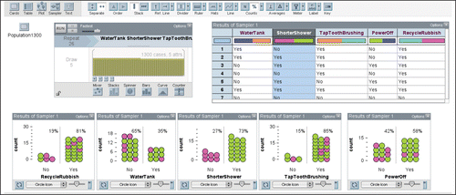
Using the (pseudo-random) Sampler in TinkerPlots, students working in pairs took a random sample the same size as the class. An example of what one of the random samples looked like for the five questions in Figure 1 is shown in Figure 2. In the figure, the Collection in the upper left corner is the ABS CensusAtSchool Population of 1300 students. For each of these 1300 students, the Sampler (next to the Population) contained the data for each of the five attributes (WaterTank, ShorterShower, TapToothBrushing, PowerOff, RecycleRubbish). The results of one such sample are shown in the Results of Sampler 1 table. Students then created five plots for the attributes, splitting the data into the “No” and “Yes” responses and labelling the percentage of each. The five “Yes” percentages were then entered into the students’ Workbooks. Using the percentages from the random samples and their own criteria again, students made decisions about the environmental friendliness of Australian Year 5 students.

Figure 2. Example of how data were collected from the ABS CensusAtSchool “population.”

For Australian Year 5 students, the students first used their class data and then their random samples to make decisions. In each case, the students expressed their confidence in the decision made. It was hence possible for students to make different decisions, with different degrees of confidence, based on the two samples. Because all random samples in the class were different, as were most of the criteria set, there was class discussion on the variation experienced and the lack both of agreement on the actual decisions and of certainty in making decisions.

4. The Extension Activity Methodology: Predicting Percentages for the Population

4.1. Participants

The participants in the activity reported here are the same as those in the study of Watson and English (2015), namely, 91 Year 5 students in four classes in one government-run school in a large Australian city. They were part of a three-year study of students’ development of understanding of beginning inference and the practice of statistics. The extension described next followed the first major activity employed in the second year of the study. The mean age of the students was 9 years, 8 months, and 48% were officially classified as having English as a second language (ESL). Only students whose parents gave written permission are included in this study. Students had participated in a major activity the previous year focussing on variation in measurement (English and Watson 2015).

4.2. Procedure

The extension activity began after a class discussion of the decisions students had made and of the variation observed in the percentages in the ABS random samples around the class. An example of one such discussion was as follows.

Teacher: …do you think [for] each group in this classroom, do you think that all of the conclusions you came up with were the same?

Chorus: No.

T: Why not? S1 [Student 1]?

S1: Because we had um different um samples.

T: Different samples and what was the other thing people were going to say? S2?

S2: Different criteria.

T: Different criteria, different samples. Now do you think each group's samples produced the same results for each question?

S3: No.

T: Why not?

S2: Because it's a randomly generated sample.

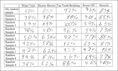
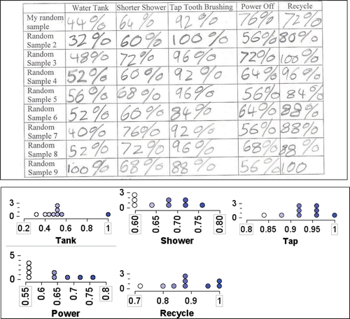
The discussion led to speculation on how these percentages might be used to predict the percentages for the ABS “population” on the five questions. After struggling to suggest combining the results from the samples, students were then asked to collect another eight random samples from the Sampler and record the percentages of “yes” responses for each of the five questions, along with the original random sample percentage values. Using the same process as previously described (see Figure 2), the students usually repeated the sample collection a total of nine times. An example of the recording from a Workbook is shown in Figure 3. Students did not have the experience to plot these values on number lines in a timely fashion.

Figure 3. Example of a table recording percentages from random samples in a student Workbook.

From the nine percentages for each attribute, students were asked to predict the “population” percentages for each attribute. As the previously completed part of the investigation had already asked for a prediction and confidence about Australian Year 5 students being environmentally friendly, the objective for the extension was to explore how the students would use the data from the nine samples to predict the ABS “population” percentage for each attribute. The procedure hence followed three stages adapted from Saldanha and Thompson's (2002) work with Year 11 and 12 students: (i) randomly select a single sample from a population and record the statistic of interest, (ii) repeat the process a large number of times, accumulating the statistics from each sample, and (iii) consider the distribution of the statistics to predict the population parameter value (in this case, the population percentage). With little experience of random sampling, it was of interest how Year 5 students would use their sample percentages to predict the population percentage.

After recording their predictions, students were asked, “Why did you choose these percentages?” This was followed by using TinkerPlots to plot the percentage of “yes” responses for each attribute in the “population” of 1300 Year 5 students. The values were recorded next to the students’ predictions in their workbooks and they were asked how close their predictions were to the population percentages and why they thought this was the case.

As most students were predicting from nine sample percentages, it was of interest to consider the strategies used to make the final predictions. The students had not been formally introduced to the mean and median but some were familiar with the mean. They had, however, been introduced to the Hat plot in TinkerPlots, where the crown of the Hat visually describes the “middle” of a dataset (Watson et al. 2008, the crown of the Hat represents the same spread as the Box of a Box plot). Students had hence had discussions about middles of datasets, as well as particular central values. It was thus of interest to observe how they would describe their predictions of the population values.

4.3. Analysis

The data used as the basis for the analysis were collected from the Student Workbooks (cf. Figure 3) after the activity was finished. Because students worked in pairs on laptops, pairs had the same recorded sample percentages. Each student, however, was expected to make his or her own prediction for the population percentage for each attribute. Because there were many different random samples, assessment of students’ predictions was quite complex. The procedure would not have been possible for students to carry out because they did not have the statistical tools or the time or experience to translate their sample values into other TinkerPlots files. The following procedure was carried out for each student's data for comparison with the predictions.

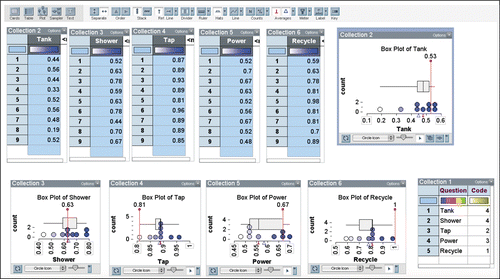
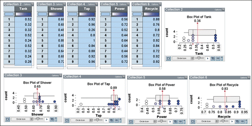
1. The sample percentages (such as the ones illustrated in Figure 3) were recorded in a spreadsheet (up to 45 values) and then (copied and pasted) in a separate TinkerPlots file for each student. This process created five collections with up to nine values (the percentages in decimal form expressed as proportions). An example is seen across the top of Figure 4.

   Figure 4. Example of file created to code predictions (vertical labeled lines) for one student.

   

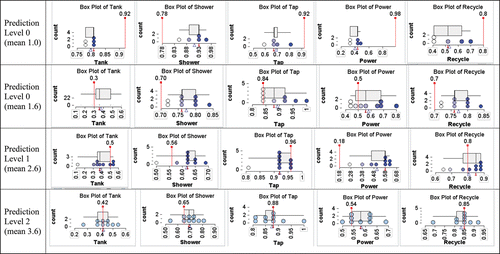
2. For each of the five collections, a plot was then created and labeled with its mean (△), median (⊥), and a Boxplot. Five plots, including Boxplots, for the five attributes are seen in Figure 4.

3. From the Student Workbooks, students’ population predictions of the percentages for the five attributes were entered as reference lines in the plots. These are seen as labeled vertical lines in each of the plots in Figure 4.

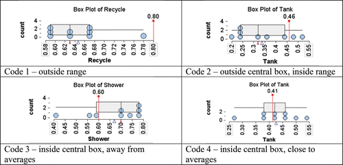
4. For each attribute predicted, a code was assigned based on the following criteria.

   • Code 1. Prediction outside the range of sample proportion values in the plot.

   • Code 2. Prediction within the range but outside of the central Box.

   • Code 3. Prediction inside the central Box but not relatively close to the mean and/or median of the sample proportions.

   • Code 4. Prediction (a) very close to the mean and/or median of the sample proportions or (b) the same as a “large frequency’’ mode (≥5 values). Rarely did this not agree with the mean and median.

     Figure 5 provides four plots that illustrate how the codes were assigned. A table with five code values for the attributes (Tank, Shower, Tap, Power, Recycle) is shown in the lower right of Figure 4.

     Figure 5. Example of plots satisfying the codes for predictions.

     

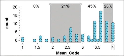
5. The code values were hierarchical and assumed to have integer properties. They were entered in the main spreadsheet for each environmentally friendly survey question, and the mean percentage was recorded for the number of questions predicted. This resulted in a distribution of means of the code values for which Prediction Levels were then defined. The highest level, Prediction Level 3, was five Code 4s or four Code 4s and a Code 3. A mean of Code 3.0–3.6 defined Prediction Level 2, showing a moderate ability to predict; Code 2.0–2.8 defined Prediction Level 1, showing a poor ability to predict, and less than 2.0 defined Prediction Level 0, indicating that the student lacked the ability to predict reasonably from the sample percentages obtained.

6. These Prediction Levels were then used in conjunction with the written responses in the Workbooks to assess the students’ explanations of why they chose their predicted population percentages. Consistency was a key to the assigning hierarchical steps. The rubric for the responses to three questions posed in relation to the random sampling is shown in Table 1. The distinction between Steps 2 and 3 responses to Q1 was related to whether or not the technique coincided with the highest Prediction Level or not. A claim of a valid technique with the lowest level of prediction was assigned Step 1 because the Prediction Level indicated that the technique had not been carried out.

   Table 1. Rubric for written responses to questions.

   Question	Step	Description
   Q1 Why did you choose these percentages?	0	No mathematical reason, e.g., “guessed,” “looking at the table”
   	1	Partial explanation without detail or inconsistent with the Prediction Level
   	2	Valid technique such as lots of, most, most common, middle, or average with Level 2 on Prediction
   	3	Valid technique such as lots of, most, most common, middle, or average with Level 3 on Prediction
   Q2 How close were your predictions of the population percentages? [Students had recorded the population values in their workbooks.]	0	No response
   	1	Qualitative description
   	2	Answer includes actual differences
   Q3 Why do you think this was?	0	No response or guess
   	1	Acknowledges poor strategy, “bad luck,” no acknowledgement of a statistical method
   	2	Acknowledges use of statistical strategy

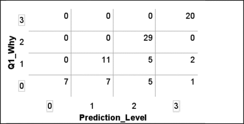
This procedure was successful in categorising the predictive capabilities of the 87 students who suggested single percentage values for the “population” for the five survey questions. Four students, however, predicted a range of plausible population percentages rather than a single percentage. Their ranges were considered separately in terms of the population percentages being included in the ranges of percentages and their final responses were considered for consistency similarly to the others. The relationship of students’ ability to predict population percentages (Prediction Level) and their explanations (Q1) for having done so was considered in a two-way table and associated indicative correlation coefficient.

5. Results

5.1. Research Question (I): How Accurate are Predictions of Population Percentages Based on Repeated Sample Percentages Made by Year 5 Students?

Figure 6 shows the distribution of the 87 means for the Codes (part 4 of procedure) of the predicted percentages for the questions posed in Figure 1. As not all students made predictions for all questions, the means were calculated based on the number completed. About 70% of students were able to make moderately good predictions (Prediction Levels 2 or 3). The Prediction Levels are highlighted in Figure 6 with alternative shading: n = 7 for Level 0, n = 18 for Level 1, n = 39 for Level 2, and n = 23 for Level 3. Examples of student predictions and their analyses for mean codes 1 and 1.6 (Prediction Level 0), 2.6 (Prediction Level 1), and 3.6 (Prediction Level 2) are shown in Figure 7. A Prediction Level 3 example is given in Figure 8.

Figure 6. Distribution of mean codes for prediction (n = 87), highlighted by prediction levels.

Figure 7. Examples of prediction levels for four different mean values of codes.

Figure 8. Example of coding of the highest prediction level.

Responses to the questions asking for explanations indicate how consistent these explanations of students’ strategies were with their predictions. The Prediction Level was taken into account when coding Q1 (cf. Table 1).

5.2. Research Question (II): What are the Levels of Reasoning Associated with Choosing the Predictions and the Explanations for Their Closeness to the Population Percentages?

5.2.1. Question 1 (Q1): Why Did You Choose These Values?

When asked why they chose the percentages written in their Workbooks, 23% of students gave no reason or reasons that included guessing, the general appearance of the percentages, or something unrelated to the data (code 0).

I choosed [chose] these percentages because I think most people choose recycle and shorter shower because its easy af[f]ordable. [ID 26]

Because I thought that most people in Australia would be okay. [ID 31]

Because we looked at the numbers. [ID 36]

Because they explain our thoughts and knowledge. [ID 54]

Australia is a big country and doesn't get much rain. [ID 85]

For code 1 responses, 21% of students only provided a partial explanation or it was inconsistent with the level of prediction.

We found w[h]ich number accured [occurred] the most. [Prediction Level 1] [ID 12]

Because what I wrote was similar to the answers to [of] our class. [Prediction Level 2] [ID 39]

We chose these percentages by looking at the results on the table above. [Prediction Level 1] [ID 82]

Since it's closest to half and it seems more accurate. [Prediction Level 1] [ID 88]

Thirty-three percent of responses were coded 2 because they provided a reasonable strategy that should have produced a high Level 3 prediction but the prediction was only moderate at Level 2.

Because these were the most common on are [our] list of data. [ID 4]

I chose these percentages because they have the most number in each attribute. [ID 28]

I chose these percentages by the most common one. [ID 49]

Because they are about the middle of the biggest percentage and smallest percentage. [ID 64]

At the highest level for Q1, coded 3, 23% of responses gave adequate strategies and these were consistent with the highest level of response for the previous prediction (Level 3).

I chose those percentages as they were the most frequent and they were in the middle. [ID 76]

The most common number. [ID 48]

Because they were the most often one in the table. [ID 32]

They were the averages of the random samples. [ID 71]

5.2.2. Question 2 (Q2): How Close Were Your Predictions of the Population Percentages?

When further asked how close their predictions were to the actual population percentages, only 3% did not respond. Twenty-nine percent of students gave qualitative descriptions of the closeness or difference (code 1).

I wasn't close at all they were at complete oppisite [opposite] ends of the chart. [ID 31]

Some I was close but some I was not close at all. [ID 15]

The prediction was very close. [ID 71]

Many students (68%), however, indicated their accuracy numerically, with lists of differences or estimations, coded 2. This was even true for students who made poor predictions (e.g., ID 22 had Level 1 predictions). For these Year 5 students, the responses were employing percentage in an ordering sense rather than as a proportion of a whole.

We were under 15% away from each proper answer. [ID 11]

Water tank: 5%; Shower: 6%; Teeth: 6%; Power off: 10%; Recycle: 6%. [ID 14]

20% to 60% away. [ID 22]

We were very close because our answers were 42, 71, 90, 82, 57 and our guesses were 42, 71, 87, 77, 59. [ID 43]

Our predictions were very close because our biggest percentage difference was only 10%. [ID 55]

5.2.3 Question 3 (Q3): Why Do You Think This Was?

Finally, students were asked the reason for their closeness or discrepancy from the population percentages. Some students did not respond and others provided confessions or nonnumerical reasons (20% at code 0).

Because I gest [guessed] them all. [ID 29]

Maybe kids are sloppier than I thought. [ID 31]

Because I looked at the numbers better. [ID 36]

We thought about it a lot. [ID 21]

At code 1, 42% of responses acknowledged using a poor strategy or perhaps having good luck, but not using a statistical method.

I think this was because of luck. [ID 13]

My estimate was very close to the real answer. [ID 14]

I think it was the strategy we used it helped a lot. [ID 56]

I think this happened because we chose the numbers correctly. [ID 69]

At code 2, responses acknowledged the use of an appropriate strategy (38%).

This was because we chose our most popular percentages for predicts. [ID 4]

I think this was because we counted which one repeated itself alot of times. [ID 52]

I think it was close because our predictions were measured from the average of the columns so this is around about what most people/kids would do. [ID 53]

Because we averaged it. [ID 71]

Our predictions were only the most common numbers and they were the best guess we had. [ID 75]

An example of a response that had the highest level of prediction for all five attributes is shown in Figure 8. The student said the mean was used to make the predictions.

For the four students who provided ranges rather than specific single population percentage predictions, two students were paired using TinkerPlots and gave ranges for two of the attributes only. These ranges included the population percentages nearly or exactly in the middle. The other two students gave ranges for all five questions and although they likely worked with TinkerPlots together, their suggested ranges were different. One included the population percentages in all five ranges, whereas the other only included three. These responses to Q2 and Q3 were assessed in relation to these range predictions and included in the analysis of codes as presented above.

Looking at the relationship of ability to make predictions and ability to explain the reasoning behind them, the correlation was 0.78. Figure 9 shows that only 23% of codes did not lie on the diagonal. The method of coding was such that it was not possible to have a more sophisticated explanation level than the level of prediction. The explanations, however, could fall short. Only 3 of 20 (15%) of the highest level of predictions did not also present high level explanations.

Figure 9. Relationship of prediction level and explanation of reasoning.

6. Discussion

The larger activity, of which this exploration was an extension, engaged students in the practice of statistics to answer a statistical question based on their class sample and a random sample from a known population. The extension went further to consider multiple random samples from the known population. The purpose of the extension was for the students to experience variation in the percentages for “yes” responses obtained from the nine random samples and to make predictions about the population percentages of “yes.” Although the class discussion focussed on variation in the random samples and estimating values in a range, students generally still suggested exact values. Teachers did not criticize this approach. The students considered the nine sample percentages for each attribute in a table but did not create a plot of values along a numerical scale, as is implied in the work of Saldanha and Thompson (2002). In relation to the first research question, the predictions for the population percentage of 71% of the students were considered at least moderately appropriate, with a mean coding over the number of survey items considered of 3.0 or higher (within the middle 50% of values, see Figure 6).

`The second research question, however, went further and considered the consistency of the reasoning justifying the predictions in relation to the actual predictions. Although some students admitted to guessing, many others displayed the modal idea of picking the most frequent value, mentioned the clustering of values, or knew how to use the mean. Overall, 56% of students predicted at least moderately well (a mean of at least three predictions “close” to the population value) combined with an explanation that employed a valid strategy for the decisions made. Fifteen percent made moderate or better predictions but did not appear to have had an appropriate strategy for doing so, and 29% struggled with the objectives of the tasks. Given the exploratory nature of this study, these percentages describe the students’ combined estimation skill and ability to explain how they were able to achieve it. The authors know of no other similar study with students this young, and hence the activity provides a starting point and the results provide a benchmark, for future research.

The second research question then considered how close the students thought their predictions were to the population percentages and why this had occurred. The level of the prediction (high or low) was not the issue here, but how well the students could describe the difference between the two percentages. Using the numerical percentages, 68% of students could describe accurately the differences, indicating that they had acquired the basic numeracy skill of comparing, ordering, and subtracting percentages in this context. Most of the rest of the students made qualitative rather than quantitative comments on the differences. Responses to the why-question showed that 38% of students could suggest they had used a strategy that could be classified as proto-statistical. For these students with limited experience carrying out statistical investigations, this was considered an encouraging result.

Informally the teachers reported how well the students accepted the use of percentage in the investigation, even though the introduction of the concept does not appear in the Australian Curriculum: Mathematics (ACARA 2015) until Year 6. In fact seeing the “Yes” and “No” complementary percentages as shown in Figure 2 was considered good explicit reinforcement of the part-whole concept for understanding percentage. The fact that more sophisticated understanding of representativeness and sample size is required for a full appreciation of the sample–population relationship (e.g., Watson and Moritz 2000; Saldanha and Thompson 2002) is the next step. These aspects were not issues for this sample of students because, for example, they had decided that the ABS “population” was a good representation of Australian Year 5 students.

It is important to comment on the four student responses from two pairs that gave ranges of possible population percentages rather than single predictions for the population percentage. These ranges are precursors to the later development of ideas related to confidence intervals. Although the responses were valued as appropriate in acknowledging variation by the teacher (in the one class where they were produced), there was no further discussion at this year level.

The idea of the relationship between the nine sample proportions collected and the theoretical distribution of all possible sample proportions, whose mean proportion is that of the population proportion was not introduced to the students. It was considered too complex for the developmental levels of the students. Recalling the difficulties that older students experience in coming to terms with this relationship (Lipson 2003; Bargagliotti et al. 2014; Watkins, Bargagliotti, and Franklin 2014), the intuitions built about basic prediction from samples may be a useful foundation when other issues, such as increasing sample size, are introduced.

Looking ahead at the Australian curriculum in Year 8 (ACARA 2015), a descriptor reads “Explore variation of means and proportions of random samples drawn from the same population” with the elaboration, “using sample properties to predict characteristics of the population” (ACMSP293). The fact that many of the Year 5 students could successfully do this for proportions leads to the hope that the intuitions developed here will be reinforced with further examples when students have more techniques and tools to use in the senior secondary years. At Level C (the highest level) of the GAISE framework (Franklin et al. 2007) “students … should understand the limitations of conclusions based on data from sample surveys … and should be able to quantify uncertainty associated with these conclusions using margin of error and related properties of sampling distributions” (p. 88). In this study, students were asked “how close?” their conclusions (predictions) were and many began to appreciate degrees of closeness, which will later become more sophisticated.

The process of providing experiences that lead to an understanding of hypothesis testing and confidence intervals based on a single random sample is exceedingly complex. Research shows that trying to put it all together at once at the senior secondary or tertiary level is fraught with difficulty (Lipson 2003; Pfaff and Weinberg 2009; Watkins, Bargagliotti, and Franklin 2014). Perhaps starting earlier with some of the basic ideas based on the foundation of variation would provide meaningful building blocks to be put together later. Although of course not all students appreciated the extension part of the activity reported here, the fact that many did may provide encouragement for further research across the middle years.

6.1. Limitations

In retrospect, it may have been easier if students had been able to view TinkerPlots graphs of the nine random samples rather than the tables that they filled in, in their Workbooks. The contrast of the basic information is shown in Figure 10. To do this, however, would have meant the creation of five new collections (one for each survey question) with nine entries made by the student pairs. Although the students had been taught how to do this in the previous year of the study, it would have been much too time-consuming, given the total length of the complete activity of which it was a part. Given the format of the Workbook, no students were seen to sketch small plots of their own.

Figure 10. Two ways of viewing the same data from nine random samples.

The activity would likely have been easier for students if there had only been one population from which to sample, based on one of the questions in Figure 1. For the main activity to be authentic, however, it was necessary for the students to consider responses to several questions in making a decision about Year 5 students being environmentally friendly. In building students’ understanding of meaningful statistical investigations, this was felt to be more important. A careful consideration of the data and results suggests that considering five questions was not a great impediment.

If introducing repeated random sampling to older students, it is likely that 20 or more random samples would be collected by students to plot and begin to see a distribution of sample means. This might have been possible if only one question were being considered, but time constraints and holding the continued interest of Year 5 students precluded this.

Finally, the criteria developed for analyzing the students’ predictions based on their random sample percentages were quite detailed, employing the mean, median, and Box plots, tools that the students generally did not use. It was not expected that they do so and using the formal measures for analysis was simply a way of easily considering the centers of the distributions efficiently, combined with the Box plots, which drew attention to the middle half of the data.

Acknowledgments

The authors acknowledge the excellent organizational support by the Senior Research Assistant, Jo Macri and helpful discussions with Christine Franklin.

Funding

This study was funded by Australian Research Council project number DP120100158.

References

- Australian Curriculum, Assessment and Reporting Authority (ACARA) (2015), The Australian Curriculum: Mathematics, Version 7.4, 30 March 2015, Sydney, NSW: ACARA.
- Bargagliotti, A. E., Anderson, C., Casey, S., Everson, M., Franklin, C., Gould, R., Groth, R., Haddock, J., and Watkins, A. (2014), “Project-SET Materials for the Teaching and Learning of Sampling Variability and Regression,” in Proceedings of IASE's 9th International Conference on Teaching Statistics (ICOTS9): Sustainability in Statistics Education, eds. K. Makar, B. de Sousa, and R. Gould, Voorburg, The Netherlands: International Statistical Institute. Available at: http://icots.info/9/proceedings/pdfs/ICOTS9_3E2_WATKINS.pdf.
- Burrill, G., Franklin, C. A., Godbold, L, and Young, L. J. (2003), Navigating through Data Analysis in Grades 9–12, Reston, VA: National Council of Teachers of Mathematics, Inc.
- Chance, B., delMas, R., and Garfield, J. (2004), “Reasoning about Sampling Distributions,” in The Challenge of Developing Statistical Literacy, Reasoning and Thinking, eds. D. Ben-Zvi and J. Garfield, Dordrecht: Kluwer, pp. 295–323.
- Common Core State Standards Initiative (2010), Common Core State Standards for Mathematics, Washington, DC: National Governors Association for Best Practices and the Council of Chief State School Officers. Available at http://www.corestandards.org /assets /CCSSI_Math%20Standards.pdf
- English, L., and Watson, J. (2015), “Exploring Variation in Measurement as a Foundation for Statistical Thinking in the Elementary School,” International Journal of STEM Education, 2, 1–20. DOI 10.1186/s40594-015-0016-x
- Franklin, C., Bargagliotti, A., Case, C., Kader, G., Scheaffer, R., and Spangler, D. (2015), The Statistical Education of Teachers, Alexandria, VA: American Statistical Association.
- Franklin, C., Kader, G., Mewborn, D., Moreno, J., Peck, R., Perry, M., and Scheaffer, R. (2007), Guidelines for Assessment and Instruction in Statistics Education (GAISE) Report: A PreK-12 Curriculum Framework, Alexandria, VA: American Statistical Association.
- Hodgson, T., and Burke, M. (2000), “On Simulation and the Teaching of Statistics,” Teaching Statistics, 22, 91–96.
- Konold, C., and Miller, C. D. (2011), TinkerPlots: Dynamic Data Exploration [computer software, Version 2.0], Emeryville, CA: Key Curriculum Press.
- Lappan, G., Fey, J. T., Fitzgerald, W. M., Friel, S. N., and Phillips, E. D. (1998), Samples and Populations, Menlo Park, CA: Dale Seymour Publications.
- Lipson, K. (2003), “The Role of the Sampling Distribution in Understanding Statistical Inference,” Mathematics Education Research Journal, 15, 270–287.
- Ministry of Education (2007), The New Zealand Curriculum, Wellington, NZ: Author. Available at http://nzcurriculum.tki.org.nz/The-New-Zealand-Curriculum.
- Moore, D. S. (1990), “Uncertainty,” in On the Shoulders of Giants: New Approaches to Numeracy, eds. L. S. Steen, Washington, DC: National Academy Press, pp. 95–137.
- Moore, D. S., and McCabe, G. P. (1993), Introduction to the Practice of Statistics (2nd ed.), New York: W. H. Freeman.
- Mulekar, M. S., and Siegel, M. H. (2009), “How Sample Size Affects a Sampling Distribution,” The Mathematics Teacher, 103, 35–42.
- Pfaff, T., and Weinberg, A. (2009), “Do Hands-On Activities Increase Student Understanding? A Case Study,” Journal of Statistics Education 17(3). Available at www.amstat.org/publications/jse_archive.htm#2009.
- Saldanha, L., and Thompson, P. (2002), “Conceptions of Sample and their Relationship to Statistical Inference,” Educational Studies in Mathematics, 51, 257–270.
- Watkins, A. E., Bargagliotti, A., and Franklin, C. (2014), “Simulation of the Sampling Distribution Can Mislead,” Journal of Statistics Education, 22. Available at http://www.amstat.org /publications /jse /v22n3 /watkins.pdf
- Watson, J. M., and English, L. (2015), “Introducing the Practice of Statistics: Are we Environmentally Friendly?” Mathematics Education Research Journal, 27, 585–613. DOI 10.1007/s13394-015-0153-z
- Watson, J. M., Fitzallen, N. E., Wilson, K. G., and Creed, J. F. (2008), “The Representational Value of Hats,” Mathematics Teaching in the Middle School, 14, 4–10.
- Watson, J. M., and Moritz, J. B. (2000), “Developing Concepts of Sampling,” Journal for Research in Mathematics Education, 31, 44–70.