Student Performance in Curricula Centered on Simulation-Based Inference: A Preliminary Report

ABSTRACT

“Simulation-based inference” (e.g., bootstrapping and randomization tests) has been advocated recently with the goal of improving student understanding of statistical inference, as well as the statistical investigative process as a whole. Preliminary assessment data have been largely positive. This article describes the analysis of the first year of data from a multi-institution assessment effort by instructors using such an approach in a college-level introductory statistics course, some for the first time. We examine several pre-/post-measures of student attitudes and conceptual understanding of several topics in the introductory course. We highlight some patterns in the data, focusing on student level and instructor level variables and the application of hierarchical modeling to these data. One observation of interest is that the newer instructors see very similar gains to more experienced instructors, but we also look to how the data collection and analysis can be improved for future years, especially the need for more data on “nonusers.”

KEY WORDS:

• Multi-level models
• Randomization tests
• Statistics education research

1. Introduction

Spurred on by George Cobb's 2005 USCOTS talk and article (2007), several groups have been developing full high school and college-level introductory statistics curricula that put tactile and technology-based simulations at the heart of helping students learn about inference, often early in the course (e.g., Lock et al. 2013; Tabor and Franklin 2013; Diez, Barr, and Çetinkaya-Rundel 2014; Forbes et al. 2014; Tintle et al. 2015; Zieffler et al. 2015). These approaches focus not on use of computer models to help students visualize statistical concepts (e.g., see Mills 2002 for a review) or on simulation-based learning (e.g., Novak 2014), but on a change in both content and pedagogy. These changes are driven by the ability to carry out standard inferential analyses (p-values and confidence intervals) through simulation rather than relying only on methods centering on the normal distribution. This also naturally facilitates a more active learning environment for the students. For example, the Tintle et al. curriculum (ISI, Introduction to Statistical Investigations) uses a coin tossing model in week 1 of the course (with physical coins and then using the computer) to introduce the logic of statistical significance before moving on to more traditional analyses (Roy et al. 2014). Introducing students to inferential reasoning through simulations and randomization tests is also part of the Common Core State Standards in Mathematics (www.corestandards.org/Math).

Although there has been anecdotal and statistical evidence of the effectiveness of this approach (e.g., Tintle et al. 2011, Tintle et al. 2012; Budgett and Wild 2014; Pfaankuch and Budgett 2014; Reaburn 2014; Stephens, Carver, and McCormack 2014; Zieffler et al. 2014; Maurer and Lock 2015), especially for lower performing students (Tintle et al. 2014), more research is needed. As part of a recent NSF grant, we have been providing workshops and support to teachers who wanted to start implementing such an approach. In this article, we examine data from the 2013/2014 academic year on several pre-/post-measures of student attitudes and conceptual understanding across a broad range of instructors at different institutions. For the broader research study, our goals are to start exploring:

1. Do gains in students' conceptual understanding substantially differ across curricula? In which topics do we see the strongest and weakest performance?

2. Are gains seen by instructors with more experience with a simulation-based curriculum as evident with instructors who are teaching such an approach for the first time?

3. Can we characterize certain instructional experiences/institutional differences/student backgrounds with higher or lower improvement?

4. How does student understanding of inference develop through repeated exposures during the course?

5. Are students able to transfer their knowledge of statistical inference to novel situations?

This article will focus mostly on goals 2 and 3. In particular, we will explore the feasibility of using cluster analysis and hierarchical linear models with cross-institutional assessment data. We recruited the authors and class-testers of the ISI curriculum at several institutions to give pre-/post-tests to their students to assess the robustness of the curriculum. We briefly address goal 1 but due to limitation with the 13/14 data, we will focus mostly on different implementations of a single curriculum. (Elsewhere, we focus on changes in student attitudes, progression of student understanding through embedded exam items within the course, and student performance on a high-level transfer question.) This is a preliminary report from our first year of data collection. It is important to remember the observational and preliminary nature of these data. We conclude with suggestions for future research and next steps in facilitating such research.

2. The Curriculum

“Simulation-based inference” has been used to describe the use of methods such as bootstrapping and randomization tests in introducing students to the logic of statistical inference. In our own curriculum we begin each chapter, including the first day of the course, with tactile and computer simulations of chance models. Subsequent topics are motivated by a six-step statistical investigation method (research question, data collection, data exploration, draw inferences, formulate conclusions, and looking back and forward) and how each step changes with different data structures (e.g., one sample, two samples, multiple samples). To draw inferences, students simulate a chance model to approximate a p-value or create a confidence interval (Chance and Rossman 2014). These simulations are performed using student-focused javascript applets from the Rossman/Chance collection through in-class, lab, and out-of-class exercises, varying by instructor. Analysis methods based on the Central Limit Theorem (e.g., z-procedures and t-procedures) are then discussed as long-run approximations to the simulation results (e.g., the applets allow the user to overlay the theoretical distribution for direct comparison). This approach moves beyond introducing students to sampling distributions through simulation, but considers simulation and randomization tests as the primary tool for carrying out inferential analyses throughout the course.

Now that textbooks exist that fully implement this approach for undergraduate introductory statistics courses, we need to be examining more data on whether and how students' attitudes and conceptual understanding are impacted by this approach. As part of an NSF grant, we are conducting professional development workshops and recruiting individuals, using and not using such a curriculum, to administer pre and post assessment tools. This development has been aided by advice from an advisory board established as part of the NSF grant (our Randomization Based Curriculum Developers, RBCD group) that has reviewed items and discussed results for validity.

3. Data Collection

3.1. Participants

Instructors were invited during Fall 2013 and Winter 2014 to participate in our assessment plan. This included instructors who helped develop the ISI curriculum, instructors who had been using simulation-based materials for several years, and instructors who were brand new to the ISI curriculum. Many instructors in the latter group participated in short professional development workshops (1 day to 4 days) offered by the ISI author team and other developers of simulation-based curricula through the NSF grant and Consortium for the Advancement of Undergraduate Statistics Education (CAUSE). Instructors were asked to submit a survey detailing how they taught the course (e.g., number of weeks, percentage of time spent on student-led experiences), though these data were incomplete. Most instructors administered both the Survey of Attitudes Towards Statistic (SATS) instrument (Schau 2003) and a concept-based inventory as pre-test at the beginning of the course and as post-tests toward the end of the course (some as review, some embedded in the final exam). Our 30-question concept inventory (see Section 3.2) was an instrument we developed using/adapting/extending items from CAOS and GOALS (Comprehensive Assessment of Outcomes in a first Statistics Course; Goals and Outcomes Associated with Learning Statistics; e.g., delMas et al. 2007; Sabbag and Zieffler 2015). In addition to these pre-/post-questions, we developed some multiple choice questions that focused on particular areas, such as student understanding of strength of evidence. The SATS instrument also includes some demographic data on the students (whether or not the course was required, GPA, major, grade level, number of previous high school or college math/stat courses, type of degree seeking, and age). Instructors were offered a small stipend for participating in the assessment program.

3.2. Concept Inventory

Our concept inventory was a modified version of the CAOS test (similar modifications were also being made resulting in the GOALS assessment). As noted in Appendix A in the online supplemental information, some questions are the same, some questions were slightly modified in context or wording, and some questions were expanded or contracted (a multiple choice vs. valid/invalid options for separate statements). Based on student performance cited by Tintle et al. (2011) as well as Fall 2012 pilot testing, we made these modifications and deleted questions that we did not feel were as discriminating of student performance (e.g., students appear to have a strong understanding of reading a scatterplot when they enter the course; students consistently struggled on an item pre- and post-test).

We also added a few items based on the following considerations:

1. Are students using a simulation-based curriculum more likely to state a large p-value is evidence in favor of the null hypothesis? (Q17)

2. Can students evaluate the strength of evidence from a study with a small p-value but also a small sample size? (Q16)

3. Can students find convincing evidence of an extreme statistic even with a small sample size? (Q35)

4. Can students compare the strength of evidence between two studies with the same statistic but different sample size? (Q36)

5. Do students realize that a sample size does not need to be excessively large in order to be considered representative of the U.S. population? (Q19)

The items and field-testing results from over 500 students from Fall 2012 were shared with the RBCD advisors before final adjustments were made. The classifications of the items was very similar to those in Tintle et al. (2011) with one graphing question and one identifying appropriate conditional proportions for comparison moved to descriptive statistics, and questions relating simulation and sampling variability questions grouped together. This gave us at least three questions in each area: Descriptive Statistics (9), Data Collection (4), Confidence Intervals (5), Tests of Significance (9), and Sampling Variability/Simulation (3). We will discuss details of student performance on these components in Section 4.3.

3.3. The Sample

Through our workshops and conference presentations, we recruited 40 instructors to participate in our assessment plan during Fall 2013−Spring 2014, with some instructors using the instruments in both fall and spring. Instructors varied in the implementation of the attitude and concept instruments (during 2013/2014 implementation these were offered as separate instruments), particularly with respect to level of incentives provided to students. For example, some instructors offered extra credit or homework or quiz credit for participation, others offered none, and some embedded the post-course concept questions in the final exam. For all but the last case, students were given the option of opting out of completing the questions but still receiving course credit.

We established minimum times for students to spend on the assessment as an exclusion criterion; if a student spent less than 3 min (or opted out) on the attitudes pre-survey or less than 10 min on the concept inventory (or opted out), those observation were removed. If student's time data were missing, we focused on whether the student responded to at least 90% of the questions on the instrument. Then, if the response rate in a section was below 40%, we removed that section from our analysis. Using these criteria, we created two datasets that were used at various points of the analysis (see Table 1). We will use the first dataset to focus on student and instructor characteristics entering the course and the second dataset to focus on student gains on the concept inventory.

Table 1. Datasets used for analysis based on participation rates.

Dataset 1: Baseline Data	Students who spent long enough on the pre-attitude survey and the concept inventory pretest and whose instructor had at least 40% class participation on the pre-tests	37 instructors (50 instructor terms), 1877 students
Dataset 2: Gains Data	Students who spent long enough on both the pre- and post-concept inventory and whose instructor had at least 40% class participation on both concept tests	24 instructors (36 instructor terms), 1116 students

For the Baseline Data, we ended up with 20 distinct instructors in the fall. In the spring, 13 of those instructors participated a second time, plus 17 new instructors. This gave us 37 distinct instructors and 50 “instructor-terms” or “sections.” This included four high school teachers and two community college teachers. The rest were four-year college (25) or research university (6) instructors. The rest were four-year college (25) or research university (6) instructors. One of the high school sections was a “dual enrollment” course allowing immediate credit at a neighboring college.

For the Gains Data, we ended up with 15 distinct instructors in the fall. In the spring, 12 of these instructors participated a second time plus 9 new instructors. This gave us 24 distinct instructors and 36 “instructor-terms” or “sections.” This included three of the high school teachers, one of the community college sections, 16 four-year college instructors, three university instructors, and the dual-enrollment section.

Though we will refer to the instructor-terms as sections for the remainder of the article, one instructor could have had multiple sections in the same term. We did not collect sufficient information to differentiate among sections within the same term but did differentiate across terms where we thought there could be more variation in implementation and experience.

4. Analyses

4.1. Instructor and Student Characteristics

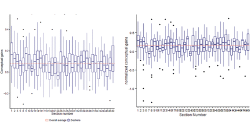
From the Gains Data, Figure 1 shows the conceptual gain (post-test–pre-test in proportion correct on the 30 concept inventory questions) for the students in each section. We also considered using a measure such as “single-student normalized gain” (e.g., Hake, 1998; Meltzer 2002; Colt et al. 2011) which focuses on the percentage of potential gain achieved, but instead will include pre-test scores as a predictor in the multi-level models. The overall average gain is only 0.084, but this is on par with the average gain seen on the similar CAOS test (delMas et al. 2007). The average normalized gain was 0.151, though with some large negative outliers (e.g., a student going from 73% correct on pre-test to 37% correct on post-test). The overall average pre-test score was 0.498 and the overall average post-test score was 0.582. We also see there is a considerable amount of student-to-student variability in the gains on the concept inventory, but also some section-to-section variability. One of our goals is to see whether we can account for some of that section-to-section variability in student conceptual gains.

Figure 1. Gains and “standardized gains” on the concept inventory by section for the 36 sections in Gains Data. The dotted line is the overall average across all the students (overall average gain = 0.084, overall average normalized gain = 0.151).

One possible explanation of the variability in the gains across sections is the level of experience of the instructor with the curriculum. In classifying the instructors by experience with the curriculum (Gains Data), we coded five as experienced instructors (e.g., author team members, some with sections both fall and spring), seven as having a “middle” level of experience (have previously used similar materials such as Introduction to Statistical Concepts, Applications, and Methods (ISCAM) more than twice), 10 as “new” instructors to the curriculum (have used the materials at most twice), and two instructors who were not using a simulation-based curriculum (e.g., Moore's Basic Practice of Statistics). One of these nonuser instructors used the assessment items in the fall and then became a new user in the spring.

The boxplots in Figure 2 illustrate that after dividing the instructors into the four experience groups (with only two nonusers), there is still considerable variability between sections in the same category (some sections with as few as five students) and relatively much less distinction between the experience categories.

Figure 2. Gains on concept inventory grouping sections by level of instructor's experience with the simulation-based curriculum.

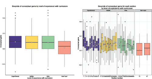
Although it is very risky to draw conclusions based on the two nonusers, there is evidence that the instructors' level of experience with the curriculum is a significant predictor of how much the students gain (p-value ≈ 0.0017). However, the R² is very small (1.3%) and a Tukey multiple comparisons only detects differences between each group with the nonuser group and not between each other.

In an effort to further explore similarities and distinctions between sections, we examined two K-means cluster analyses: one on student characteristics and one on instructor characteristics. We wanted to see whether some classroom environments were similar enough to each other to be pooled together and whether these clustering variables would explain much variation in student gains.

Using the Baseline Data, 13 student level variables included age, GPA, grade level (0 = high school, 1 = lower division college, 2 = upper division college), number of previous high school math/stat classes, number of previous college math/stat classes, sex (0 = male, 1 = female), pre-concepts performance, and the six scales from the attitudes pre-test. Looking at the student averages across the sections (and seeing where the within and between subject sums of squares balance), we find four clusters (Table 2).

1. Cluster 1 (8 sections, 4 in Gains Data): Sections that generally had more previous high school and college mathematics courses and highest pre-concept scores, more positive attitudes coming into the course, including the perceived value of statistics. Higher proportion of women and upper classmen compared to the other clusters.

2. Cluster 2 (5 sections, 4 in Gains Data): HS and community college sections with fewer previous math and statistics courses but similar pre-concept scores on average. Generally more positive attitudes coming into the course. Higher proportion of women than the other clusters.

3. Cluster 3 (29 sections, 22 in Gains Data): Sections with lower GPAs, lower division college students on average.

4. Cluster 4 (8 sections, 6 in Gains Data): Sections with generally more negative attitudes coming into the course and expected to put in more effort. More likely to be male.

Table 2. Variable means for student cluster analysis.

	Age	GPA	Grade	Previous HS	Previous college	% fem	Pre concepts	Affect	Cog conf	Value	Diff*	Interest	Effort*
1	21.20	3.40	1.57	3.67	2.29	43%	0.55	4.55	5.07	5.54	3.76	5.23	6.29
2	16.94	3.61	0.81	3.00	0.15	50%	0.48	4.52	4.92	4.94	3.91	4.77	5.94
3	19.81	3.25	1.22	3.78	0.84	38%	0.48	4.11	4.71	5.06	3.64	4.70	6.10
4	21.72	3.32	1.48	3.70	1.24	21%	0.44	3.69	4.45	4.78	3.43	4.44	6.38

*Lower scores on effort imply the student does not plan to have to work as hard in the course; lower scores on difficulty (Diff.) imply the student perceives the course will be difficult.

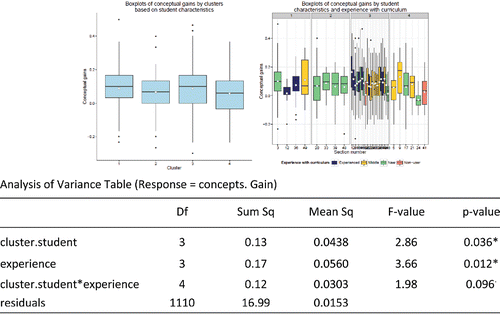
Figure 3 examines the gains on the concept inventory by the end of the course and compares those scores across these four clusters. There is some evidence of differences in the average conceptual gains between the clusters (p-value = 0.037), but with only cluster 3 significantly different (higher gains) than cluster 4 (Tukey's HSD p-value = 0.049). Less than 1% of the variation in student gains can be attributed to the student clusters. We can also consider evidence of a ceiling effect as cluster 1 had higher concept scores to begin with (we consistently found a negative association between pre-concept score and gains in concept score as discussed below). It is interesting to note that including the instructor's level of experience in the model is significant, but the p-value for student cluster does not change much and the interaction between these terms is weakly significant.

Figure 3. Grouping sections by student characteristics (one-way ANOVA p-value = 0.037).

A similar cluster analysis was done based on instructor level characteristics. However, more than half of the instructors did not complete the instructor survey. This resulted in a usable dataset of 19 instructors across 30 sections (1212 students).

First, we separated out the high school teachers. Then, the six variables used for classifying college sections based on instructor characteristics were type of department (1 = statistics, 0 = other), tenure status (1 = tenured, 0 = untenured), years of teaching, what percentage of class time was “student-led” rather than “instructor-led” (self-reported from the instructor survey), length of class weeks (1 = half-term, 2 = quarter, 3 = semester), and sex of instructor. Table 3 shows the results of the cluster analysis.

1. Cluster 1 (2 sections): This is a half-semester course taught by an experienced female in a mathematics department.

2. Cluster 2 (9 sections; 5 in Gains Data): These are statistics department faculty on the quarter system.

3. Cluster 3 (16 sections, 14 in Gains Data): These are math department faculty teaching semester-long courses. They tend to have more years of teaching and less student-led class time.

4. Cluster 4 (10 sections, 9 in Gains Data): Similar to cluster 3 but slightly less experience and more student-led class time (though still less on average than clusters 1 and 2).

Table 3. Variable means for instructor cluster analysis.

	Dept	Tenure	Avg years teaching	Avg % student led	Avg length of term	Instructor sex
1	All nonstat	0% tenured	20.0	65.0	1	100% female
2	All stat dept	44% tenured	14.0	43.9	2.1	78% female
3	All nonstat	100% tenured	18.9	32.8	3.0	25% female
4	All nonstat	0% tenured	12.2	36.5	2.9	20% female

The high school and dual-enrollment sections will be considered as cluster 5 (3 sections in Gains Data). The instructor sex may be a proxy for other variables (e.g., most of the instructors on the quarter system were female), but there has also been some interest in the role of instructor gender on student achievement (e.g., Friend 2006; Thomas 2006; Dee 2007; Antecol, Eren, and Ozbeklik 2012), mostly at lower grade levels.

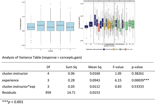
Figure 4 shows the conceptual gains for these five clusters. Overall the post-test performances in the clusters look very similar, and there are still substantial within cluster differences among sections.

Figure 4. Boxplots of conceptual gains by instructor level clusters.

The following output examines the instructor cluster effects after adjusting for the instructors' level of experience with the curriculum. This model and the one-way ANOVA model (not shown) indicate that the clustering by instructor-variables is not useful to the model, with or without the level of experience variable.

In examining our cluster-based groupings, we find that the instructors' level of experience with the curriculum is the most significant, though we still need to be cautious with the very small number of sections of nonusers in this dataset. After adjusting for the instructors' level of experience with the curriculum, we do have a marginally significant relationship with the student level clusters. However, we do not find significant effects from the instructors' clusters after adjusting for the instructors' level of experience. We also did not have sufficient response rate on the instructor survey (variables like student-led percentage), so subsequent analyses will not consider the instructor clusters, but will only consider some individual instructor level variables that we could verify independently, namely instructor sex, type of school (high school, community college, 4-year college, research university), length of term, and level of experience with the curriculum.

4.2. Hierarchical Models

Next, we explored additional models in an attempt to explain section-to-section variability in student conceptual gains. We used hierarchical modeling to include student and instructor level variables in a same model, and to account for the correlation between students who are within the same section (e.g., Gelman and Hill 2006). The unconditional means model (or random-intercept model which compares the mean gains across the 36 sections in the Gains Data) found an intraclass correlation coefficient of 0.006, implying the section-to-section variability only accounts for 0.6% of the total variability in student conceptual gains. If we remove the nonusers from the dataset, this coefficient drops to 0.002. These results suggest that it will be difficult to find variables at the section level that account for significant variability in student performance, though adjusting for other variables may still reveal some patterns.

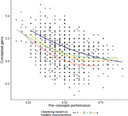
Several regression models were explored using MCMCglmm in R version 3.1.2 using the Gains Data. (We also explored lmer but had more problems with convergence. We did use lmer for factor p-values in our final models.) As mentioned previously, one of the strongest predictors of students' gain (post–pre concepts scores) is the pre-concept score. We do find some evidence of a negative quadratic association (see Figure 5, with separate curves for the four student level clusters).

Figure 5. Scatterplot of conceptual gains versus pre-concept performance by student clusters.

This negative association suggests that students who know more coming into the course tend to not learn as much as in the course, with higher scores for student cluster 1 (more prepared, more positive pre-attitudes) and lower scores for cluster 4 (lower pre-attitudes) after adjusting for pre-concept performance. Whereas the overall post-test scores are strongly related to pre-test scores, we see a quadratic effect where the gains are larger for the students with lower pre-test scores. For more analysis of the performance of lower-performing students, see Tintle et al. (2014).

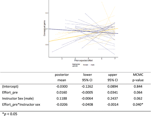
To illustrate a hierarchical model, below is a model for predicting conceptual gains based on the students' pre-attitude of the effort they plan to spend on the course and the instructor sex. The Effort variable is the sum of the student's responses across four questions (e.g., “I will study hard for every statistics test”), with higher effort scores indicating the student plans to work harder in the course. So we can model the gain for student j with instructor i as${\text{gain}}_{ij}={\beta }_{0i}+{\beta }_{1i}{\text{effort}}_{ij}+{ϵ}_{ij},$where we are going to allow the intercepts and the slopes to vary across instructors. So for example, we could think of the intercepts as varying based on the instructor's sex:${\beta }_{0i}={\beta }_{00}+{\beta }_{01}\text{instructor}{\text{sex}}_i+{ϵ}_{0i},$and the slopes (the relationship between effort and gain) as also varying based on the instructor's sex:${\beta }_{1i}={\beta }_{10}+{\beta }_{11}\text{instructor}{\text{sex}}_i+{ϵ}_{1i}.$

Putting these equations together, the hierarchical or multilevel model has the following form:$\begin{array}{l}{\text{gain}}_{ij}={\beta }_{00}+{\beta }_{01}\text{instructor}{\text{sex}}_i+{\beta }_{10}{\text{effort}}_{ij}\\ +{\beta }_{11}\text{instructor}{\text{sex}}_i\times {\text{effort}}_{ij}+{ϵ}_{1i}{\text{effort}}_i+{ϵ}_{0i}+{ϵ}_{ij}.\end{array}$

Figure 6 shows the section-to-section variability in the conceptual gains versus planned effort as well as solid “pooled” regression lines from the hierarchical model (weighting by sample size etc.) for male and female instructors.

Figure 6. Scatterplot of conceptual gains versus prior expected effort by instructor sex.

From the solid lines, we see that the overall association in our dataset is slightly negative for the male instructors and positive for the female instructors. This could indicate a different impact of planned effort on conceptual gains. For example, with female instructors, students who plan to work hard in the course tend to gain more in the course, but not with male instructors. It could also be an indication of other confounding relationships as well.

As another example, Figure 7 shows the individual and pooled relationships between gain and prior Affect scores separated by the instructors' level of experience with the curriculum. Affect is a measure of students' “feelings concerning statistics” (Schau 2003). Larger values indicate a more positive opinion of statistics (e.g., “I will like statistics”).

Figure 7. Scatterplot and hierarchical model of conceptual gains versus prior affect by instructor curriculum experience.

Figure 8. Predicting student gains from student clusters and instructor level variables.

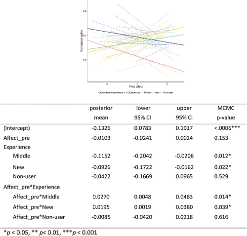
We see that students who have a higher appreciation of Statistics coming into the course tend to have higher gains for the middle and new instructors, but less for the experienced and nonusers of the curriculum.

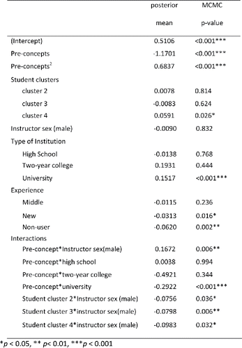
We applied this multi-level modeling approach using the student cluster variable and the four instructor level variables (student cluster, instructor sex, type of school, and level of experience with curriculum). We also included the student pre-concept scores (quadratic) as that appears to be a highly significant variable on its own. We included interaction terms between pre-concepts and instructor sex, pre-concepts and school type, pre-concepts and level of experience, and student cluster and instructor sex. After applying a backwards elimination process (using a 0.15 cut-off), the output in Figure 8 shows the signs of the coefficients and their p-values.

The significant variables in predicting student gains on the concept inventory appear to be

1. A negative quadratic (concave up) association with pre-concept scores.

2. The negative effect of pre-concepts is smaller (flatter) for male instructors than for female instructors (Figure 9(a) for illustration), but larger for students at two-year colleges (Figure 9(b)). In other words, male and female instructors tended to see similar gains for students with low pre-test scores but female instructors tended to see lower gains for students with high pre-test scores compared to male instructors. Whereas community college students tended to see lower gains, especially among the students with higher pre-test scores.

   Figure 9. (a) Gain on concept inventory versus pre-test showing overall male/female instructor lines; (b) gain versus pre-test separated by type of institution; (c) comparison of gains for male/female instructors across the four student clusters.

   

   Figure 10. Predicting student gains from student clusters and instructor level variables.

   

3. Higher gains for student cluster 1 (more prepared, more positive pre-attitudes), especially with male instructors, yet in the other clusters, the gains tended to be lower for male instructors. (See Figure 9(c) for the unconditional boxplots.)

4. The student cluster effect stems primarily from cluster 4 (lower pre-attitudes, mostly male students), with higher gains in cluster 2 (HS and community college students with less background) and cluster 1.

5. Experienced users had higher gains with average gains decreasing with less instructor experience with the curriculum and the lowest gains on average with the nonusers.

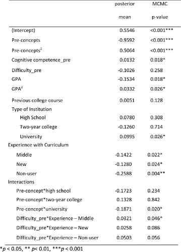
Finally, we looked at the individual student-level variables and the three instructor-level variables. We also tested interactions between the pre-concepts scores and individual attitude scales, pre-attitude scales with instructor level of experience, student age by sex, and pre-effort by instructor sex. With backwards elimination, none of these interactions were statistically significant at the 0.05 level in the final model. The closest was difficulty × instructor experience (factor p-value = 0.089). The final model, including this one interaction, is shown in Figure 10. The intraclass correlation coefficient of this model is 0.051, indicating that just 5% of the unexplained variation can be attributed to differences in sections.

The significant variables appear to be

1. A negative quadratic (concave up) association with pre-concept scores.

2. Higher gains on average for students who had higher cognitive confidence pre-test scores (believing they can learn the material).

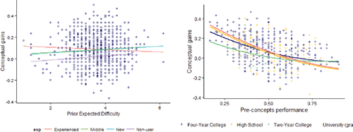
3. Students who expected the course to be less difficult tended to have higher gains except with the more experienced instructors, for which expected difficulty was not really related to gains. (Figure 11(a)).

   Figure 11. (a) Gains versus prior expected difficulty by level of experience with curriculum; (b) gains versus pre-concepts by school type.

   

   Figure 12. Comparison of pre-/post-scores for an instructor who switched to the simulation-based curriculum between fall and spring semesters.

   

4. A quadratic (concave up) relationship with GPA. Students with GPAs above 3.0 are predicted to see higher gains.

5. Two-year college students who score lower on the pre-test have lower gains compared to the other institution types, but the higher performing students on the pre-test tend to have slightly lower gains on the post-test for university and high school students (Figure 11(b)).

6. Lower gains on average for instructors with less (or no) experience with the curriculum.

4.3. Item-by-Item Performance

Appendix A shows the pre- and post-test percentages for students within each type of instructor experience. If the item was similar to a CAOS item that is noted in the table along with the CAOS normative data as reported in Tintle et al. (2011). Table 4 shows the average percentage correct of the questions (shown in parentheses) in each sub-topic on the pre-test (with standard deviations) and the average gain in the percentage correct. Coming into the course (pre-test during week 1), students performed strongest on the data collection questions. The students in simulation-based curricula showed the largest gains on the tests of significance and confidence intervals questions.

Table 4. Categorizations of concept inventory questions (means and standard deviations) separated by instructor level of experience with curriculum.

	Pre-test				Gain
	Exp	Mid	New	Non	Exp	Mid	New	Non
Data collection (4)	0.643 (0.232)	0.631 (0.231)	0.634 (0.229)	0.593 (0.273)	0.019 (0.312)	−0.103 (0.313)	0.021 (0.305)	−0.050 (0.302)
Descriptive statistics (9)	0.484 (0.235)	0.435 (0.215)	0.475 (0.228)	0.461 (0.212)	0.079 (0.212)	0.075 (0.244)	0.069 (0.209)	−0.020 (0.209)
Sampling variability (3)	0.424 (0.304)	0.371 (0.275)	0.411 (0.297)	0.357 (0.256)	0.110 (0.331)	0.062 (0.343)	0.055 (0.390)	0.016 (0.341)
Confidence intervals (5)	0.446 (0.195)	0.438 (0.210)	0.429 (0.194)	0.414 (0.220)	0.093 (0.264)	0.139 (0.267)	0.115 (0.274)	0.056 (0.259)
Tests of significance (9)	0.588 (0.180)	0.559 (0.187)	0.586 (0.197)	0.504 (0.189)	0.119 (0.229)	0.118 (0.255)	0.100 (0.252)	0.054 (0.264)

Several observations are worth noting:

1. (Q7) Students continue to struggle with a question asking them to choose a histogram over case-value plots as most informative in examining shape, center, and spread of the distribution, frequently picking a symmetric shape.

2. (Q9) When students were asked a pointed question that would identify a low response rate as a concern for generalizability, the students in the simulation-based curricula performed worse on the post-test compared to the pre-test.

3. (Q10–13) Small gains are seen across the confidence interval questions, more so for the simulation-based curricula.

4. (Q16) Performance on a question related to issues of power was worse on the post-test compared to the pre-test.

5. (Q17) Students do exhibit a tendency to find an insignificant result to be evidence in favor of the null hypothesis.

6. (Q19) Students continue to perform poorly on a question asking them to ballpark a sample size necessary for a specified margin-of-error.

7. (Q20) Students on the simulation-based curricula far out performed other students on a post-test question asking whether a larger or small p-value is desirable.

8. (Q21–23) But performance is more inconsistent when asked to identify incorrect p-value interpretations. Just under 50% consider a p-value interpretation as the probability of the alternative as valid.

9. (Q24–26) Students did not perform well on questions asking them to match a histogram with a verbal description of a variable.

10. (Q31) On the post-test, less than half could identify a correct description of a simulation (and invalidate others) but this was still marked improvement from the pre-test.

11. (Q35) When asked to evaluate a result of 12 successes out of 14 attempts, students were evenly split in choosing “random chance,” “some evidence,” and “strong evidence” against random chance.

4.3.1. The Flipper

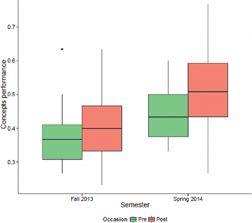
One instructor in our dataset used the assessments in Fall 2013 and then again in Winter 2014, after changing to the simulation-based curriculum. In looking at the concept inventory as a whole (Figure 12), this instructor saw significantly higher gains in the second semester. The gains (not shown) appeared to be highest for the Data collection and Confidence interval questions.

5. Discussion

This study has provided an example of using hierarchical models to explore the relationship of various variables on student achievement in an introductory statistics course across multiple institutions. The preliminary analysis is consistent with earlier evidence on the potential of centering the course on simulation-based inference, but also raises questions and suggestions for future research, particularly about the relative impact of student-level and instructor-level variables on student performance across different curricula. This study has also revealed several areas for improvement, both in how we are assessing the students and also identifying the content students are finding most difficult.

After adjusting for pre-attitude measures, pre-concept score, and a few other student- and instructor-level variables, we do find evidence that students in a nonsimulation-based curriculum tended to achieve lower gains on our concept inventory than students in such a curriculum. However, we must keep in mind the limited number of nonuser sections in this dataset. We also find some evidence of higher gains for students with more experienced instructors, but those effects are smaller and the “middle” experience instructors are similar to the “new” instructors. This provides some evidence of the robustness of the curriculum to instructors trying it for the first time. Instructors willing to switch to a simulation-based curriculum should immediately see similar gains as more experienced instructors.

The most significant predictors of student gains are the students' pre-test scores, with students scoring lower on the pre-test achieving higher gains on average, and student GPA coming into the course. Of the pre-attitudes, prior beliefs of cognitive competence and difficulty seemed to be the better predictors, with similar coefficients. The higher gains for students with higher GPAs and more positive attitudes entering the course is consistent with student clusters 1 and 2 achieving higher gains on average. Students who enter the course expecting it to be more difficult and expecting to need to put in lots of effort into the course tend to not perform as well. Instructors may be well served to discuss expectations and possibilities with students at the beginning of the course. Although these data point to potential impacts of institutional differences, instructor pedagogical choices, and other student level variables, including prior attitudes, our next steps focus on obtaining additional and more diverse data to further comment on these and other factors (e.g., a priori quantitative majority, race, etc.).

Student-level variables appear to have more impact than the individual instructor-level variables that we had available in this initial dataset. However, there is some evidence that the impact of these variables differs between male and female instructors. Some of the interactions we observed may be proxies for other things (e.g., most of the Statistics Department instructors in our dataset were female, on the quarter system, and among the more experienced users of the curriculum). More data are needed to be able to separate such confounding variables. Similarly, we are not able to distinguish between the change in sequencing of ideas, focus on simulation-based content, and the inevitable active learning pedagogy from heavier use of simulations. However, it appears that these potential interactions merit further investigation and that multi-level modeling appears a feasible way to capture such cross-level relationships. It is important to understand the role of instructor–student interactions on the impact of different curricula.

In examining the questions that students showed less improvement on, one theme seems to be the role of sample size. Students are still exhibiting some confusion on when they can have strong evidence with small sample sizes, how sample size is related to generalizability, and how sample size relates to power. The emphasis of this curriculum on ideas of statistical inference is evident in those areas showing more improvement. As seen in Tintle et al. (2011), gains on descriptive statistics questions are more modest, though students are showing stronger background on those questions entering the course. We do conjecture that one reason for lower performance on the question of matching standard deviations to graphs is inconsistency in how the answers are labeled and how the graphs are labeled (e.g., answer option A to choose graph C).

Further research will explore in more detail the development of student understanding throughout the course. Some instructors have noted slow transfer of inferential thinking in the first few topics, raising the questions of how much repeated exposure is necessary for students to develop a deep understanding of statistical significance and which experiences are most critical for student learning. For example, students seem to struggle longer than we might expect to know what “observed result” to use when calculating the p-value (vs. the hypothesized parameter value). Perhaps giving students interesting data and then asking them to carry out simulations does not sufficiently illustrate to students the distinction between “real” versus “hypothetical” data. Having students carry out more of the studies themselves and having a statistic they actually observed themselves may help keep the real data from becoming abstract (e.g., Gould 2010; Kuiper and Sturdivant 2015).

6. Next Steps

We have collected similar data for the 2014–2015 school year with 76 instructors at over 40 institutions. We have improved our process in the following ways:

1. Combining the concept inventory and attitude questions into one assessment. We are hoping this will help with response rate though more students may decide to not complete the instrument in one sitting.

2. Replacing the “number of previous math and statistics courses” questions with a question simply asking whether they have taken a previous statistics course.

3. Creating separate forms for different instructors to reduce erroneous identification, though we still need to check for repeat names and mismatches on the pre-/post-test.

4. Rephrasing of questions on the instructor survey and more aggressive follow-up to ensure complete and accurate instructor responses.

5. Most importantly, more efforts to recruit nonusers as well as instructors using other simulation-based curricula.

We have also made a few changes to the concept inventory:

1. The problematic histogram/case-value plot question is no longer the first question on the instrument.

2. We reordered the answer options in Questions 33 and 34 so the graph choice matches the forced choice (e.g., a refers to Graph A, b refers to Graph B, etc.).

We have added additional questions:

1. Rather than allowing “all of the above” to the descriptions of a simulation, this has been broken into several valid/invalid statements.

2. Duality of confidence interval and test of significance.

3. Two questions on factors that impact width of confidence intervals.

4. Comparing strength of evidence across several pairs of dotplots.

5. Drawing cause-and-effect conclusion when random assignment is present in study design.

6. An invalid p-value interpretation related to the difference in conditional proportions.

In addition to these pre-/post-comparisons, we have also developed a series of “common questions” for instructors to use on midterm exams throughout the term. For example, in year 1, we focused on student understanding of the simulation process (data to be analyzed). In year 2, we will focus on more in depth assessment of student understanding of confidence intervals. We have also developed a high-level transfer question that can be used on the final exam. This is an adaptation of the 2009 AP Statistics question that expects students to evaluate skewness by considering a sampling distribution of the mean/median statistic. After using several iterations of this question as an open-ended question, we are now pilot testing a multiple choice version for broader implementation.

7. Summary

Using multi-level regression models, we conducted an initial exploration of the impact of both student-level and instructor-level variables on the performance of students in 36 different sections of introductory statistics at 23 different institutions. In the models we explored, the student-to-student variability far exceeded the section-to-section variability. How much the students knew coming into the course and how confident they feel about their ability to learn the material appear to be stronger predictors of how much they learn regardless of instructor characteristics. However, it would be worth exploring additional interactions. Additionally, we were not able to identify predictors that explained a large percentage of this student-to-student variability. We have made slight adjustments to our instrument and increased our efforts to recruit nonusers of simulation-based curricula and instructors using other simulation-based curricula to participate in our assessment, which will include assessments of students' growth in understanding at different points of the term as well as a high-level transfer question.

Supplementary Materials

Supplemental data for this article can be accessed on the publisher’s website.

Acknowledgments

The authors would like to thank Roxy Peck and Karen McGaughey for comments on earlier drafts of this article.

Funding

This work was carried out as part of NSF DUE grant #1323210.

References

- Antecol, H., Eren, O., and Ozbeklik, S. (2012), “The effect of Teacher Gender on Student Achievement in Primary School: Evidence from a Randomized Experiment,” IZA Discussion Paper No. 6453, Institute for the Study of Labor (IZA). Available at http://ftp.iza.org/dp6453.pdf
- Budgett, S., and Wild, C. (2014), “Students' Visual Reasoning and the Randomization Test,” in Proceedings of the 9th International Conference on Teaching Statistics, Flagstaff, AZ. Available at http://iase-web.org/icots/9/proceedings/pdfs/ICOTS9_8A1_BUDGETT.pdf
- Chance, B., and Rossman, A. (2014), “Using Simulation-Based Inference for Learning Introductory Statistics,” WIREs Computational Statistics, 6, 211–221.
- Cobb, G. (2007), “The Introductory Statistics Course: A Ptolemaic Curriculum?” Technology Innovations in Statistics Education, 1, Available at http://escholarship.org/uc/item/6hb3k0nz
- Colt, G. C., Davoudi, M., Murgu, S., and Zamanian Rohani, N. (2011), “Measuring Learning Gain During a One-day Introductory Bronchoscopy Course,” Surgical Endoscopy, 25, 207–216. Available at http://www.ncbi.nlm.nih.gov/pmc/articles/PMC3003781/#CR13
- Dee, T. (2007), “Teachers and the Gaps in Student Achievement,” Journal of Human Resources, 42, 528–554.
- delMas, R., Garfield, J., Ooms, A., and Chance, B. (2007), “Assessing Students' Conceptual Understanding After a First Course in Statistics,” Statistics Education Research Journal, 6, 28–58. Available at http://www.stat.auckland.ac.nz/∼iase/serj/SERJ6%282%29_delMas.pdf
- Diez, D., Barr, C., and Çetinkaya-Rundel, M. (2014), “Introductory Statistics with Randomization and Simulation,” CreateSpace Independent Publishing Platform, Available at OpenIntro.org.
- Forbes, S., Chapman, J., Harraway, J., Stirling, D., and Wild, C. (2014), “Use of Data Visualization in the Teaching of Statistics: A New Zealand Perspective,” Statistics Education Research Journal, 13, 187–201. Available at http://iase-web.org/documents/SERJ/SERJ13%282%29_Forbes.pdf
- Friend, J. (2006), “Research on Same Gender Grouping in Eighth grade Science Classrooms,” Research in Middle Level Education, 30, 1–5.
- Gelman, A., and Hill, J. (2006), Data Analysis Using Regression and Multilevel/hierarchical Models, New York, NY: Cambridge University Press.
- Gould, R. (2010), “Statistics and the Modern Student,” International Statistical Review, 78, 297–315.
- Hake, R. R. (1998), “ Interactive Engagement Versus Traditional Methods: A Six-Thousand Student Survey of Mechanics Test Data for Introductory Physics Courses,” American Journal of Physics, 66, 64–74. Available at http://www.physics.indiana.edu/sdi/
- Hake, R. R. (2002), “ Normalized Learning Gain: A Key Measure of Student Learning” (Addendum to Melzer, D. E. (2002), “The Relationship Between Mathematics Preparation and Conceptual Learning Gains in Physics: A Possible ‘Hidden Variable’ in Diagnostic Pretest Scores),” American Journal of Physics, 70, 1259–1267.
- Kuiper, S., and Sturdivant, R. (2015), “Coaching Students to Address the Challenges of Reproducible Research,” submitted to The American Statistician, 69, 354–361.
- Lock, R., Frazer Lock, P., Lock Morgan, K., Lock, E., and Lock, D. (2013), Statistics: Unlocking the Power of Data, New York: Wiley.
- Maurer, K., and Lock, E. (2015), “Bootstrapping in the Introductory Statistics Curriculum,” Technology Innovations in Statistics Education, 9. Available at http://escholarship.org/uc/item/0wm523b0.
- Meltzer, D. E. (2002), “Normalized Learning Gain: A Key Measure of Student Learning,” Addendum to Melzer, D. E. (2002), “The Relationship Between Mathematics Preparation and Conceptual Learning Gains in Physics: A Possible ‘Hidden Variable’ in Diagnostic Pretest Scores,” American Journal of Physics, 70, 1259–1267.
- Novak, E. (2014), “Effects of Simulation-Based Learning on Students' Statistical Factual, Conceptual and Application Knowledge,” Journal of Computer Assisted Learning, 30, 148–158.
- Pfannkuch, M., and Budgett, S. (2014), “Constructing Inferential Concepts Through Bootstrap and Randomization-Test Simulation: A Case Study,” in Proceedings of the 9th International Conference on Teaching Statistics, Flagstaff, AZ. Available at http://iase-web.org/icots/9/proceedings/pdfs/ICOTS9_8J1_PFANNKUCH.pdf
- Reaburn, R. (2014), “Introductory Statistics Course Tertiary Students' Understanding of p-Values,” Statistics Education Research Journal, 13, 53–65. Available at http://iase-web.org/documents/SERJ/SERJ13(1)_Reaburn.pdf
- Roy, S., Rossman, A., Chance, B., Cobb, G., VanderStoep, J., Tintle, T., and Swanson, T. (2014), “Using Simulation/Randomization to Introduce p-value in Week 1,” in Proceedings of the 9th International Conference on Teaching Statistics, Flagstaff, AZ. Available at http://icots.info/9/proceedings/pdfs/ICOTS9_4A2_ROY.pdf
- Sabbag, A. G., and Zieffler, A. (2015), “Assessing Learning Outcomes: An Analysis of the GOALS-2 Instrument,” Statistics Education Research Journal, 14, 93–116. Available at http://iase-web.org/documents/SERJ/SERJ14(2)_Sabbag.pdf
- Schau, C. (2003), “Survey of Attitudes Toward Statistics (SATS-36),” available at http://evaluationandstatistics.com/
- Stephens, M., Carver, R., and McCormack, D. (2014), “From Data to Decision-Making: Using Simulation and Resampling Methods to Teach Inferential Concepts,” in Proceedings of the 9th International Conference on Teaching Statistics, Flagstaff, AZ. Available at http://iase-web.org/icots/9/proceedings/pdfs/ICOTS9_8B3_STEPHENS.pdf
- Tabor, J., and Franklin, C. (2013), Statistical Reasoning in Sports, New York: W.H. Freeman and Company.
- Thomas, D. S. (2006), The Why Chromosome: How a Teacher's Gender Affects Boys and Girls, Stanford, CA: Education Next.
- Tintle, N. L., Chance, B., Cobb, G., Rossman, A., Roy, S., Swanson, T., and VanderStoep, J. (2015), Introduction to Statistical Investigations. New York: Wiley. Available at http://math.hope.edu/isi
- Tintle, N., Swanson, T., VanderStoep, J., Roy, S., Rossman, A., Cobb, G., Rogers, A., and Chance, B. (2014), “Quantitative Evidence for the User of Simulation and Randomization in the Introductory Statistics Course,” in Proceedings of the 9th International Conference on Teaching Statistics, Flagstaff, AZ. Available at http://icots.info/9/proceedings/pdfs/ICOTS9_8A3_TINTLE.pdf
- Tintle, N., Topliff, K., VanderStoep, J., Homes, V.-L., and Swanson, T. (2012), “Retention of Statistical Concepts in a Preliminary Randomization-Based Introductory Statistics Curriculum,” Statistics Education Research Journal, 11, 21–40. Available at https://www.stat.auckland.ac.nz/∼iase/serj/SERJ11%281%29_Tintle.pdf
- Tintle, N., VanderStoep, J., Holmes, V-L., Quisenberry, B., and Swanson, T. (2011), “Development and Assessment of a Preliminary Randomization-Based Introductory Statistics Curriculum,” Journal of Statistics Education, 19, available at http://ww2.amstat.org/publications/jse/v19n1/tintle.pdf
- Zieffler, A., and Catalysts for Change (2015), Statistical Thinking: A Simulation Approach to Uncertainly (3rd ed.), Minneapolis, MN: Catalyst Press.
- Zieffler, A., delMas, R., Garfield, J., and Brown, E. (2014), “The Symbiotic, Mutualistic Relationship Between Modeling and Simulation in Developing Students' Statistical Reasoning About Inference and Uncertainty,” in Proceedings of the 9th International Conference on Teaching Statistics, Flagstaff, AZ. Available at http://iase-web.org/icots/9/proceedings/pdfs/ICOTS9_8B1_ZIEFFLER.pdf