Strategies for Using a Spatial Method to Promote Active Learning of Probability Concepts

Abstract

We developed and tested strategies for using spatial representations to help students understand core probability concepts, including the multiplication rule for computing a joint probability from a marginal and conditional probability, interpreting an odds value as the ratio of two probabilities, and Bayesian inference. The general goal of these strategies is to promote active learning by introducing concepts in an intuitive spatial format and then encouraging students to try to discover the explicit equations associated with the spatial representations. We assessed the viability of the proposed active-learning approach with two exercises that tested undergraduates’ ability to specify mathematical equations after learning to use the spatial solution method. A majority of students succeeded in independently discovering fundamental mathematical concepts underlying probabilistic reasoning. For example, in the second exercise, 76% of students correctly multiplied marginal and conditional probabilities to find joint probabilities, 86% correctly divided joint probabilities to get an odds value, and 69% did both to achieve full Bayesian inference. Thus, we conclude that the spatial method is an effective way to promote active learning of probability equations.

Keywords:

• Bayesian inference
• Multiplication rule
• Spatial cognition

1 Introduction

Probability concepts are a cornerstone of Science, Technology, Engineering, and Math (STEM) education, especially in the many fields that rely on statistical methods to draw conclusions. Unfortunately, people are prone to many fundamental misunderstandings of probabilistic reasoning, so educators face a strong headwind when they attempt to teach these concepts. The cognitive psychology literature documents many of these confusions, such as thinking that conjunctions of features can be more likely that the individual features themselves (Tversky and Kahneman 1983) or erroneously transposing conditional probabilities (Diaconis and Freedman 1981). The high risk of confusion is likely exacerbated by the fact that probability concepts are usually taught using mathematical notation that is unfamiliar to many students, so exploring more intuitive representations is a promising approach for improving understanding.

The current article discusses strategies for using spatial representations of probability concepts in statistics instruction. We present evidence that many students can succeed in active-learning activities that challenge them to translate spatial representations into symbolic equations. As detailed below, we explored spatial methods for (1) distinguishing marginal, conditional, and joint probabilities; (2) finding a joint probability from a marginal and conditional probability (i.e., the multiplication rule); (3) finding an odds value by dividing two probabilities; and (4) Bayesian inference. The first three concepts are common elements of undergraduate statistics courses, and Bayesian inference is quickly becoming an important part of the statistics curriculum (Martinez and Achar 2014). Bayesian inference is also a central concept in various STEM subject areas such as naïve Bayes algorithms in computer science (Koski and Noble 2009) and diagnostic test interpretation in medicine (Gigerenzer and Hoffrage 1995).

1.1 Background

Without training, people are typically poor at probabilistic reasoning, a fact that is perhaps most clearly illustrated by studies on Bayesian reasoning. Bayesian inference is the process of combining probabilistic evidence sources to determine what is likely to be true. Bayesian reasoning experiments typically explore this ability by presenting word problems that challenge participants to find the probability that some hypothesis is true given that some observation has been made.

Solving Bayesian reasoning problems requires basic probability skills that are common learning objectives for undergraduate statistics courses, such as distinguishing marginal, conditional, and joint probabilities and applying the multiplication and addition rules for combining probabilities. Experiments investigating Bayesian reasoning typically use problems with two hypotheses (e.g., a patient has a disease not) and a dichotomous observed variable (e.g., a positive or negative diagnostic test for the disease), which is the simplest version of Bayesian inference and a good starting point for courses that cover Bayesian statistics (Kruschke 2011).

Following this formula, a classic Bayesian reasoning example is finding the probability that a patient has a disease (hypothesis) given that they get a positive diagnostic test (observation). Problems typically report the proportion of cases overall for which the hypothesis is true (e.g., the base rate of the disease in the general population), the proportion of hypothesis-is-true cases that are consistent with the observation (e.g., the proportion of people with the disease who get a positive test result), and the proportion of hypothesis-is-false cases that are consistent with the observation (e.g., the proportion of people without the disease who get a positive test result).

A clear finding in this literature is that most people cannot perform the probabilistic reasoning needed to answer Bayesian reasoning questions; instead, they tend to rely on heuristics (Gigerenzer and Hoffrage 1995; Cohen and Staub 2015) or prior knowledge (Cohen, Sidlowski, and Staub 2017). Simplifying the problem by providing nested frequencies helps (e.g., Gigerenzer and Hoffrage 1995), but still leaves solution rates around 24% compared to 4% when problem information is presented as percentages/proportions (McDowell and Jacobs 2017). Other changes in problem format can also impact success rates. For example, Böcherer-Linder and Eichler (2019) reported success rates of 60–75% when the elements of frequency-format problems were presented as a contingency table compared to 20–50% when the problem elements were presented as a tree diagram. Expanding the tree diagram to include all values in the contingency table—what the authors call a double-tree diagram—improved performance relative to standard tree diagrams, but still left accuracy rates substantially below the contingency table format. Unit squares and icon arrays, which represent probabilities with the areas of rectangles, also fell short of contingency tables, although icon arrays produced performance levels similar to contingency tables for 3 out of their 4 word problems.

The wide variability in effectiveness across formats reported by Böcherer-Linder and Eichler (2019) is representative of the literature as a whole. Generally, studies have found that providing visual representations of Bayesian inference problems can improve performance, but some display formats are not effective (Cosmides and Tooby 1996; Sloman et al. 2003; Yamagishi 2003; Brase 2009, 2014; Micallef, Dragicevic, and Fekete 2012; Sirota, Kostovièová, and Juanchich 2014; Binder, Krauss, and Bruckmaier 2015; Böcherer-Linder and Eichler 2017, 2019; Wu et al. 2017; Reani et al. 2018). Clearly, more work is needed to determine the relative effectiveness of these approaches. In particular, not all proposed representations have been thoroughly compared, including, for example, “truth tables” that enumerates the logical relationships between hypotheses and observations (Satake and Vashlishan Murray 2015).

Researchers have also explored systematic, instructional programs for Bayesian inference. Sedlmeier and Gigerenzer (2001) investigated computer-based tutorials to compare the effectiveness of three instructional approaches. Rule-based training taught participants to directly input the probabilities reported in the problem into the Bayes’ theorem equation. Frequency-grid training taught participants to translate the probabilities reported in the problem into frequencies and mark components of an icon array to represent these frequencies. Frequency-tree training was similar to the frequency grid, except that participants were taught to enter frequencies as numbers in a tree diagram. Although all of these training versions improved Bayesian inference performance, the frequency versions produced more durable learning, as assessed by follow-up sessions weeks or months after the initial training.

Kurzenhäuser and Hoffrage (2002) investigated instructional programs similar to the rule-based and frequency-based training from Sedlmeier and Gigerenzer (2001) in an in-person classroom setting. The frequency-based, or “representation,” training taught participants to solve Bayesian problems by translating probabilities to frequencies and filling in contingency tables and tree diagrams with those frequencies. A delayed test that came months after training showed a clear advantage for representation training over rule-based training.

One consistent characteristic of effective visual displays is that they represent probabilities with simple spatial features such as length (Wu et al. 2017). Starns et al. (2018) developed an instructional program for Bayesian inference that capitalizes on this spatial advantage. In a six-minute video, participants were taught how to perform approximate Bayesian inference using a spatial representation devised by a participant in Gigerenzer and Hoffrage (1995). In four laboratory experiments, they showed that undergraduate students can quickly learn this spatial method, resulting in a dramatic improvement in their performance on Bayesian reasoning problems. A classroom sample also showed clear performance improvements after training in this spatial method.

1.2 The Current Project

The current project explores the potential for using the spatial method from Starns et al. (2018) as an instructional aid in statistics courses that cover basic probability concepts. The spatial method could have unique advantages that complement the approaches described in the previous section. Most critically for the current purposes, the spatial method provides a way to demonstrate key probability concepts and have students work through problems without relying on equations. Thus, this method provides a more accessible and intuitive introduction to Bayesian reasoning and related probability concepts. Although an intuitive understanding is valuable in itself, students in a statistics course would also need to learn to work with equations, of course. Thus, an important question is whether students can relate an intuitive spatial understanding of probability concepts to explicit equations.

We will focus on a particularly ambitious goal for linking spatial representations and equations; specifically, teaching students with the spatial method and then challenging them to discover the associated equations in an active-learning exercise. Basic research from psychology shows that self-generated information is remembered much better than passively viewed information (Slamecka and Graf 1978), so students who succeed in discovering the mathematical analogs of the spatial techniques should experience substantial learning benefits. Moreover, pre-exposure to the spatial representations can help all students meaningfully interpret the symbols in equations when they later receive direct instruction on mathematical procedures (see Section 2.2). Indeed, the opportunity to correct misconceptions can provide a rich learning experience even for students who initially apply the wrong equations (Wiggins 1998). Beyond these likely learning benefits, educational research shows that students prefer active-learning activities to passive lecturing (Freeman et al. 2014). Thus, educators have many good reasons to develop techniques that promote active-learning success.

Starns et al. (2018) reported a cursory evaluation of students’ ability to translate the spatial method into explicit equations. Specifically, in the last phase of the classroom activity, students formed small groups and worked together to try to specify how each step of the spatial technique could be translated into a mathematical equation. Over 80% of the groups succeeded, suggesting that a meaningful proportion of individual students can discover the mathematics of probabilistic reasoning after learning the spatial technique. However, succeeding at the group level requires only a single group member with the correct answer, and it is possible that information was sometimes shared across groups in this relatively uncontrolled setting. Thus, the classroom sample does not rule out the possibility that only a small subset of students discovered the required math and relayed this information to their classmates.

In summary, the results from Starns et al. (2018) highlight the possibility that the spatial technique is a good way to promote active learning by presenting initial problems in an intuitive format and providing students with a chance to discover the link between these representations and the associated equations. Our goals for the current article are to discuss strategies for using spatial representations in classroom instruction on probability concepts and to test whether a substantial proportion of students can independently discover mathematical equations after learning the spatial method. To obtain more accurate estimates of the proportion of students who can succeed at this task, we assessed individual performance instead of group work in a classroom setting.

In Section 2, we outline techniques for using spatial displays in probability instruction. In Sections 3 and 4, we present results from two studies that tested whether participants could translate the spatial method into equations. Finally, we discuss future directions in the practice of using spatial representations to illustrate probability concepts.

2 Instructional Strategies

2.1 Probabilistic Reasoning Without Equations

In this section, we show how spatial representations can help students conceptually understand probability concepts before they are confronted with equations. This strategy offers educators the opportunity to convey key concepts without eliciting potentially negative reactions to mathematical content. For this initial discussion, readers should try to understand the general principles without concern for exact mathematical solutions.

Consider the following problem:

The police need to find a potential witness to an accident. The witness was seen driving a pickup truck, and the police are considering whether or not they should focus their search in a nearby rural community. 10% of residents in their jurisdiction live in the rural community, and 90% do not. 45% of residents in the rural community drive a pickup truck, compared to 10% of residents who do not live in the rural community.

In traditional Bayesian reasoning studies, one might be asked to provide the probability that the witness lives in the rural area (hypothesis) given that they drive a truck (observation). The current study used multiple question prompts in line with our interest in evaluating more basic probability concepts in addition to Bayesian inference. For example, in one of our active-learning exercises we used prompts with the following structure:

• What is the probability that a resident lives in the rural community and drives a truck?

• What is the probability that a resident does NOT live in the rural community and drives a truck?

• Given that the witness drives a truck, is it more likely that the witness lives in the rural community or not?

• How many times more likely?

Problems of this sort are usually solved by applying equations, but they are also amenable to a spatial solution method that could be more intuitive for many people (Starns et al. 2018). Figure 1 represents the population of residents in this jurisdiction, with bar lengths corresponding to the information reported in the problem. The total lengths of the bars show the total proportions of residents who do and do not live in the rural community, 10% and 90%, respectively ( “∼” means “not” in this context). The relative length of the bars shows which hypothesis is more likely overall and how many times more likely. Here, it is more likely that a resident does not live in the rural area; moreover, this possibility is nine times more likely than the possibility that the witness does live in the rural area. In other words, for every resident who lives in the rural community there are nine residents who do not (the Rural bar fits into the Not Rural bar nine times). This ratio of two probabilities is a statistical concept called odds, and in the context of Bayesian inference this is called the prior odds because it represents a situation before new information is learned.

Fig. 1 Example showing the spatial method for assessing the hypotheses that a witness does or does not live in a rural area (“Rural” and “∼Rural,” respectively) based on the observation that the witness drives a pickup truck. See text for further details.

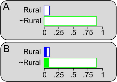
Information about the type of vehicle is represented by filling in the bars with the proportion of residents who drive a pickup truck, as in Figure 1(B). The “Rural” bar is filled to 45% of its total length, and this filled part represents people who both live in the rural community and drive a pickup truck. The “Not Rural” bar is filled to 10% of its total lengths to represent people who do not live in the rural community but do drive a pickup truck. By evaluating the length of these filled portions of the bars relative to the full x-axis (i.e., all residents), one can determine the proportion of residents who live in the rural area and drive a truck (blue filled bar) and the proportion of residents who do not live in the rural area and drive a truck (green filled bar). These are the probabilities requested in the first two questions in our four-question sequence.

One can determine which hypothesis is more likely to be true given the observation by comparing the length of the filled bars. Here, there are more residents who do not live in the rural community and drive a pickup truck than residents who do live in the rural community and drive a pickup truck (the bottom filled portion is longer than the top filled portion), so it is more likely that a pickup truck-driving resident does NOT live in the rural community than that they do (Question 3). The relative length of the filled portions shows the posterior odds, that is, the odds after the observed information is considered. In this case, the filled part of the “Not Rural” bar is twice as long as the filled part of the “Rural” bar, revealing a posterior odds value of 2:1 in favor of the Not Rural hypothesis.

In summary, although driving a pickup truck is certainly more characteristic of people who live in the rural community, this new evidence was not strong enough to overturn the very uneven base rates indicating that a small proportion of residents overall live in the rural community. The bar display highlights all of the relevant inputs, making it obvious that the relative lengths of the filled bars are influenced by both the lengths of the original bars and the proportion of each bar that are filled. Thus, creating the display discourages common fallacies of probabilistic inference that involve disregarding one or more of the relevant factors, like the base-rate fallacy (e.g., Bar-Hillel 1980), the prosecutor’s fallacy of confusing the compliment of the false positive rate for the posterior probability (Thompson and Shumann 1987), or simply confusing the true positive rate and the posterior probability (Gigerenzer and Hoffrage 1995; Cohen and Staub 2015).

This spatial display provides a way to help students understand the essence of Bayesian inference without using equations: New information changes the odds that a hypothesis is true because it rules out some of the possibilities. The full bars represent all possibilities (before new information arrives), the open part of the bars represents the possibilities that are ruled out by the new information, and the filled part of the bars represents the possibilities that are consistent with the new information. In the current example, once the police consider the observation that the witness drives a pickup truck, they should disregard all other residents and just focus on pickup drivers. That is, updating beliefs in response to the observed information simply means switching from looking at the full bars to focusing on just the filled portions. Having a simple spatial representation of the logic of Bayesian inference should be particularly helpful for students who are unlikely to glean the basic principle just from studying equations. Below, we will discuss how elements of the spatial display have a one-to-one mapping to terms in the Bayes’ theorem equation, but we also wish to emphasize that creating the spatial display can stand alone as an (approximate) solution method.

There are many ways that educators can use this sort of spatial representation to help students build an intuition for the purpose and logic of probabilistic reasoning before introducing any equations. Here, we will make a few suggestions. Perhaps the most basic strategy is simply showing students a number of displays and asking them to provide approximate answers based on interpreting the display. This is a good way to quickly go through a number of different scenarios, because judging bar lengths takes a lot less time than reading word problems and attempting to solve them mathematically. The initial displays could even be presented without any corresponding numbers, which encourages students to focus on deeper conceptual aspects of the problem situation (Givven et al. 2019). To challenge students a bit more, one possibility is to give them verbal descriptions of scenarios and ask them to draw corresponding bar displays. The scenarios could be things like “You start out thinking the hypothesis is likely to be true but seeing the observation makes you think it is likely to be false” or “You start out with no idea whether or not the hypothesis is true or false and seeing the observation makes you strongly believe that it is true.” In a large lecture class, this could be transformed into a multiple-choice question (“Which of these four bar displays is consistent with the given scenario?”) so students could use an electronic student-response system.

2.2 Linking Equations to Spatial Representations

A major advantage of the spatial technique is that components of the display have a one-to-one correspondence with elements of Bayes’ theorem, the equation for performing Bayesian inference. Moreover, elements of the display have a direct link to related probability concepts that are standard topics in statistics courses. In this section, we use the pickup truck example to link the spatial method to explicit equations. Our goal is to demonstrate how educators can buttress understanding of the equations with a supporting structure that students might find more intuitive. Figure 2 shows spatial representations and mathematical notation for four core probability concepts: (1) distinguishing marginal, conditional, and joint probabilities; (2) the multiplication rule; (3) finding an odds value by dividing probabilities; and (4) Bayesian inference. The example starts with the simplest concept in Row 1 and builds in complexity as one moves down the rows.

Fig. 2 Illustration of the link between the spatial method and explicit equations for a range of probability concepts, using the pickup truck problem as an example. Each row introduces a new concept with increasing levels of complexity, and the panels in the row show how the concept is represented in the spatial display and in mathematical notation. “Rural” and “∼Rural” represent the hypotheses that the witness does and does not live in a rural area, respectively. See text for details.

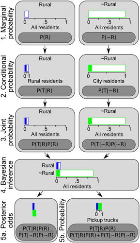
Marginal probability (Row 1) is the probability of observing one level of a variable out of a full population, ignoring all other variables. For example, in Figure 2, P(R) denotes the probability of living in the rural community and P(∼R) denotes the probability of not living in the rural community. These values apply to all residents in the jurisdiction without regard to any other variable (e.g., pickup truck ownership). In the spatial display, marginal probabilities are represented by total bar lengths. Here, the “Rural” bar goes to.1 because P(R) = 0.1 and the “Not Rural” bar goes to 0.9 because P(∼R) = 0.9.

Conditional probability (Row 2) is the probability of observing a certain level of one variable for a given level of another variable. In this case, we need to consider the probability of driving a pickup truck (denoted with “T”) given that a resident lives in the rural community, P(T$|$R), and the probability of driving a pickup truck given that a resident does not live in the rural community, P(T$|\sim$R) (“$|$” means “given” in this context). The critical concept here is that specifying a condition restricts the population to a certain subset. Thus, the axes in these panels end at the end of the bars, because we are considering only the residents in the Rural or Not Rural categories, respectively. A conditional probability is represented by the filled portion of a bar. Here, we fill in 45% of the Rural bar because P(T$|$R) = 0.45 and 10% of the Not Rural bar because P(T$|\sim$R) = 0.10.

Joint probability (Row 3) is the probability of a combination of multiple variables (e.g., both a rural community resident and a pickup truck owner) out of a full set (e.g., all residents). The mathematical procedure for finding joint probabilities is called the multiplication rule. Here, taking 45% of the 10% of rural residents leaves 4.5% of residents overall who both live in the rural community and own a pickup truck [P(T$|$R)P(R) = 0.45 × 0.1 = 0.045], and taking 10% of the 90% of nonrural residents leaves 9% of residents overall who do not live in the rural community but do drive a pickup truck [P(T$|\sim$R)P(∼R) = 0.1 × 0.9 = 0.09]. Rather than an abstract formula, the bar representation translates the multiplication rule into an explicit spatial mechanism. The third row of Figure 2 displays the logic of this step by placing the filled bars from Row 2 on the axis representing all residents. On this full axis, the filled parts of the “Rural” and “Not Rural” bars end at 0.045 and 0.09, respectively. Comparing Rows 2 and 3 reveals that the only difference between conditional and joint probabilities is the scale. For joint probability, we are back to considering all residents, not just rural or nonrural residents. In other words, we are back on the original x-axis.

One ambitious strategy for capitalizing on the direct link between the spatial representation and the equation for the multiplication rule is to show students the spatial method for finding a joint probability (fill in a bar representing the marginal probability proportional to the conditional probability) and challenge them to figure out how that translates into a mathematical equation. The exercises below investigate whether a substantial proportion of students can succeed in this task. Even if an instructor does not want to take this active-learning approach, supplementing discussion of the multiplication rule with the spatial technique could help students understand why multiplying the marginal and conditional probabilities results in the joint probability. In particular, multiplying by a decimal cuts the original value down to a proportion of its value. The marginal probability gives the proportion of cases that meet Condition A (total bar length) and multiplying by the conditional probability of B given A limits this set to just those that also meet Condition B (filled bar length).

Finally, comparing joint probabilities achieves Bayesian inference, as shown in Rows 4 and 5. Row 4 puts both hypotheses on the same axis to create the spatial display discussed above (Figure 1(B)). The equations in Row 5 are the odds version (5a) and probability version (5b) of Bayes’ theorem as applied to the pickup truck example. Notice that both equations are simply new arrangements of the joint probabilities from Row 3. Working with only the joint probabilities means that we have discarded all of the possibilities that are inconsistent with the observed information to create a new reference population (only residents who drive a pickup truck). For the left panel, the fact that the Not Rural bar is twice as long as the Rural bar visually displays the posterior odds of 2:1 in favor of the hypothesis that the witness does not live in the rural area.

Mathematically, the posterior odds are calculated by dividing one joint probability by another; for example, dividing the joint probability for “Not Rural and Truck Driver” by the joint probability for “Rural and Truck Driver” gives the “2:1 against” value evident in the display (0.09/0.045 = 2). For the right panel, all that has happened is that the Rural and Not Rural joint probabilities (the filled bars) are combined on the same axis for comparison. The fact that the blue part of the bar goes up to 1/3 on the axis reveals that the posterior probability of Rural is 1/3, or about 33%. In other words, out of all the residents who drive pickup trucks, 1/3 of them live in the rural community. The corresponding equation answers this question: “Out of all the residents who drive a pickup truck, what proportion of them live in the rural community?” This can be found by dividing the 4.5% of residents who both live in the rural community and drive a pickup truck by the 13.5% of residents overall who drive a pickup truck. The latter value is found by taking the 4.5% of rural, truck-driving residents and adding in the 9% of nonrural, truck-driving residents.

Again, one strategy for using the link between the spatial display and the Bayes’ theorem equation would be to show students the spatial method of finding posterior odds (look at how many times longer one joint-probability bar is than the other) and challenge them to specify the corresponding mathematical procedure (divide one joint probability by the other). The exercises below test whether a substantial proportion of students can independently discover the math required to find the posterior odds after learning the spatial technique. Although not tested here, a similar procedure could be used for posterior probabilities to see if students can translate the spatial solution method (look at the proportion covered by each joint probability bar when they are stuck together) to an equation-based method (divide each joint probability by the sum of both joint probabilities).¹ Educators could also decide to forego this active-learning approach but still supplement instruction on equations with the spatial representations to help students intuitively understand what the equations achieve.

3 Active-Learning Exercise 1

We have suggested that educators use spatial representations in initial instruction on probability concepts and then give students the chance to discover the associated mathematics in an active-learning process. We imagine that most educators would only want to attempt this if they can expect that a substantial proportion of their students will succeed in the active-learning challenge. The goal of this exercise was to test whether or not this is the case. As mentioned above, Starns et al. (2018) showed that a strong majority (>80%) of small groups of undergraduate statistics students were able to correctly specify the mathematics associated with applying the spatial display in an active-learning exercise. This result is promising, but the classroom setting makes it difficult to rule out the possibility that only a small subset of students succeeded in the active-learning exercise and then shared the information with their peers. Accordingly, for the current exercise undergraduate students attempted the active-learning task as individuals.

Exercise 1 was completed as part of author WL-R’s undergraduate honors thesis project. College undergraduates were tutored in the spatial method for solving probabilistic reasoning problems in one-on-one sessions, and then they completed a “math induction” worksheet that presented the visual solution to a problem and asked participants to specify the equations associated with each step. The example problem involved determining the odds that a student knows how to read music given that they own an instrument. Similar to the pickup-truck problem above, participants were given the base rate of students overall who know how to read music, the probability of owning an instrument for students who know how to read music, and the probability of owning an instrument for students who do not know how to read music. The worksheet also included a bar display for the problem that had the filled parts of the bar labeled with letters, as shown in Figure 3.

Fig. 3 The problem and bar display on the math induction sheet for Exercise 1.

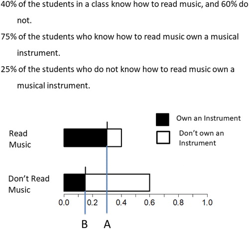
Participants were asked three questions: “Mathematically, how do you figure out where the shaded region of the ‘Read Music’ bar ends on the x-axis (marked by the letter A)?”; “Mathematically, how do you figure out where the shaded region of the “Don’t Read Music” bar ends on the x-axis? (marked by the letter B)?”; and “Mathematically, how do you figure out how many times longer the shaded region is for ‘Read Music’ than ‘Don’t Read Music’?” We will refer to the first two questions as the “Multiplication Rule” questions and score each participant as correctly applying the multiplication rule if they multiply the appropriate marginal and conditional probabilities on both questions. We will refer to the third question as the “posterior odds” question and score it correct if the participant divides the joint probabilities computed in questions 1 and 2.

3.1 Methods

3.1.1 Participants

We recruited 23 undergraduate students from the psychology department’s participant pool. One participant was removed from analyses because the instructor mistakenly revealed the math before the math induction sheet (this was the first participant run by that instructor). Participants received extra credit in their psychology classes as remuneration.

3.1.2 Procedure

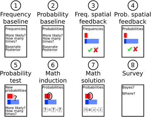
The exercise consisted of six steps summarized in Figure 4. Each step was presented to participants as an individual worksheet.

Fig. 4 Summary of the worksheet sequence in Exercise 1. See text for a description of each step.

When participants arrived, they were first asked to read and sign the consent form. The form allowed the participants to indicate whether or not they consented to having their session audio recorded, and 19 participants granted permission for recording. The primary purpose of the recordings was to ensure that proper instruction procedures were followed by the undergraduate researchers who conducted the sessions. A graduate student reviewed all of the recordings to ensure that the instructor never revealed the math linked to the spatial method before having the participant complete the math induction sheet. As mentioned in Section 3.1.1, one instructor did reveal the math in the first session that he conducted, and data from this session were removed from analyses. The audio recordings are available on the OSF (https://osf.io/aq7w3/?view_only=ccb6dc5b367e419facc7965b3a0caaf5).

After signing the consent form, participants began the sequence of six worksheets summarized in Figure 4. All worksheets involved Bayesian reasoning problems that asked participants to assess the hypothesis that a student in a class knows how to read music given the observation that the student owns an instrument (scans of responses on all worksheets from all participants are available on OSF, https://osf.io/aq7w3/?view_only=ccb6dc5b367e419facc7965b3a0caaf5).

The first and second worksheets asked participants to solve problems without any training to establish baseline performance. The first worksheet (“Frequency baseline”) presented the following problem:

• In a class, 10 of the students know how to read music and 40 do not.

• Out of the 10 who know how to read music, 8 own a musical instrument and 2 do not.

• Out of the 40 who do not know how to read music, 4 own a musical instrument and 36 do not.

Participants reported the prior and posterior odds associated with the problem in four steps. First, they were asked to consider a student in the class without knowing whether or not this student owned an instrument and select whether the student was more likely to know how to read music or not. Second, they were asked how many times more likely the option they selected was than the other option. Responses to those two questions together constituted the prior odds. Third, they were asked to consider another student in the class who owns an instrument and select whether the student was more likely to know or not know how to read music. Fourth, they were asked how many times more likely the option they selected was than the other option. Responses to the third and fourth questions constituted the posterior odds. After the participant recorded all responses, the instructor provided quick feedback on the problem (more formal feedback was provided during the frequency feedback worksheet described below). The feedback simply noted the different numbers that need to be compared for any general student from the class and for a student who owns an instrument (e.g., “There are 8 students who own an instrument and read music and 4 students who own an instrument and do not read music, so there are twice as many students who do know how to read music in this set.”).

The second worksheet (“Probability baseline”) was very similar to the first, except that it presented a new problem in probability format:

• 10% of the students in a class know how to read music, and 90% do not.

• 45% of the students who know how to read music own a musical instrument.

• 20% of the students who do not know how to read music own a musical instrument.

The participants were asked to report the prior and posterior odds that a student from this class knows how to read music in the same four-step sequence as the first worksheet. No feedback was provided for this worksheet, because answering the probability format questions involved the same math that we later tested with the math-induction task.

After completing the first two worksheets, participants received instruction based on the spatial solution method. Instruction began with a feedback sheet that covered the frequency-format problem from the first worksheet (“Freq. spatial feedback”). The feedback sheet included the original problem text along with a bar display representing the problem information. The instructor explained that the total bar lengths represented all the students who could and could not read music (top and bottom bars, respectively) and the filled parts of the bars represented the students who owned an instrument. The instructor reinforced this by pointing out that the end of the two full bars and the two filled portions matched the corresponding numbers in the problem text. The feedback sheet also had the same questions as the first worksheet, but this time with the answers filled in. The instructor explained how the answers could be discovered by looking at the bar display; namely, that the answers to questions 1 and 2 could be found by noting which of the two full bars was longer and estimating how many times the shorter bar could fit into the longer one and that the answers to questions 3 and 4 could be found by following the same procedure with just the filled portions of the bars. Participants were not told how to derive the correct answers mathematically.

Instruction continued with a sheet that presented the same problem as the frequency baseline and the frequency feedback sheet, but this time in a probability format (“Prob. spatial feedback”). The instructor compared the two problems to show that they contained the same information in different formats. The sheet displayed a bar representation of the problem information, and the instructor again explained what each component of the display represented. The instructor also noted that the bar display looked exactly the same as the one for the frequency format problem other than a change in the x-axis. The answers were again filled in, and the instructor again reviewed the procedure for finding the answers with the bar display. As before, the instructor did not provide information on the mathematical equations needed to find the correct answers.

The training culminated with a new probability-format Bayesian inference problem that gave participants a chance to implement the spatial solution method with guidance from the instructor (“Probability test”). The problem text was at the top of the page, and a blank bar display appeared just below it. Participants were asked to draw bars that would represent the information in the problem. After their attempt, the instructor helped them correct any mistakes they made to create a display that matched the problem, if necessary. The participant then answered the same four questions from the previous worksheets using the spatial display, with help from the instructor, if needed. The instructor only provided guidance in applying the spatial method to answer the questions. No instruction was provided on how to find the answers with mathematical equations.

Next, participants were asked to complete the math induction worksheet (“Math induction”). Participants were shown the same Bayesian problem from worksheet two, but this time accompanied by a corresponding bar display. Participants were first asked how to mathematically calculate the shaded regions of both the displayed bars; that is, the joint probabilities. Each question had a fill-in-the-blank format, with two blank spaces for the numerical components of the equation, one blank space for a mathematical operation (addition, subtraction, multiplication, or division), and one blank space for the resulting answer. A correct answer required entering the appropriate marginal and conditional probabilities from the problem for the numbers and multiplication for the math operation. We will collectively call the first two items the “multiplication rule questions,” and we scored this component as a success if the participant entered the correct equation for both items. A third question asked participants to write a mathematical equation to find how many times longer one shaded region was than the other; that is, the posterior odds. Here too, the question was given as a fill-in-the-blank format requiring numerical values and a mathematical operation. A correct response required entering the two joint probabilities calculated in the first two questions for the numerical components and entering a division sign for the math operation. We will call the third item the “posterior odds” question.

After the participant completed the math induction sheet, the instructor collected it and then explained how to find the correct answers (“Math solution”). The instructor also asked the participant if they had ever seen problems like the ones from the exercise and if so, where they had seen them (“Survey”).

3.2 Results

As in past research (e.g., Gigerenzer and Hoffrage 1995), we found higher success rates for untrained Bayesian reasoning problems presented in a nested-frequency format compared to a conditional-probability format. Specifically, 45% of our participants correctly specified both the prior and posterior odds for the frequency-format problem compared to just 14% for the probability-format problem. To make inferences about population success rates, we used Bayesian parameter estimation with a prior distribution that assigned equal likelihood to all probability values (a Beta distribution with shape parameters of 1 and 1). Credible intervals for the frequency (90% CI [0.30, 0.62]) and probability (90% CI [0.06, 0.30]) formats did not overlap, supporting high confidence that the difference between the two is not attributable to sampling variability.

In contrast to the low success rate for the initial probability-format problem (14%), over half (55%) of participants succeeded on all of the math induction questions after learning the spatial method. Broken down by question type, 73% of participants succeeded for both of the multiplication-rule items and 59% succeeded for the posterior odds item. Bayesian estimates of population success rates ruled out the possibility that only a small proportion of students are able to succeed in this sort of active learning exercise. Specifically, our results are consistent with population success rates of 0.54 (90% CI [0.38, 0.70]) for correctly answering all math induction questions, 0.71 (90% CI [0.55, 0.85]) for correctly answering the multiplication rule questions, and 0.59 (90% CI [0.42, 0.74]) for correctly answering the posterior odds question.

Success rates on the math induction task were encouragingly high. Nearly 3/4 of the students in Exercise 1 multiplied the appropriate conditional and marginal probabilities to find joint probabilities, and inferential tests support high confidence that the population success rate is above 50% (0.98 of the posterior distribution was above this value). Thus, educators can expect that a majority of students will succeed in this aspect of the math-induction task after training in the spatial method. Results were not as strong when it came to discovering that one needs to divide the joint probabilities to obtain the posterior odds, with a slim majority of students succeeding in this task and weaker evidence that the population success rate is above 50% (0.80 of the posterior distribution was above this value). One of the goals for Exercise 2 was to see if we could amend the procedures to increase success rates for the posterior odds question.

4 Active-Learning Exercise 2

We reviewed the session recordings from Exercise 1 to see if we could clarify the process of finding the posterior odds based on spatial relationships. The resulting changes are described in detail in Section 4.1.2, but for now we will highlight a few of the biggest changes. First, the Exercise 2 training phase began with a problem that the instructor (author JMV) solved by creating the bar display and noting the spatial relationships needed to answer the questions. The instructor carefully explained each component of the display as he created it and emphasized the process of estimating the posterior odds by imagining how many copies of the shorter filled section could fit into the longer filled section. We hoped that this would help participants thoroughly understand each component of the display by seeing the step-by-step process of creating the bars as opposed to getting a feedback sheet with the full display already visible as in Exercise 1. Second, we asked participants to directly estimate the joint probabilities from the spatial display during the spatial training, as opposed to just having them estimate the prior and posterior odds as in Exercise 1. We hoped that having rough values for these components would help participants gain insight into how they could mathematically produce the posterior odds that they see in the spatial display.

A secondary goal for Exercise 2 was to estimate baseline performance on the math induction task. We designed the math induction task to test whether students can translate the spatial method into equations, but doing so involved breaking the problem into steps that are each linked to a component of the spatial display. This “road map” might enhance performance on its own. This would be important to know, because it would mean that educators can implement a successful active-learning procedure without the need to teach the spatial solution method (although the spatial method could have other benefits besides supporting successful active learning, of course). In Exercise 2, we explored the impact of breaking the problem into steps by asking participants the math-induction questions both before and after they learned the spatial method.

Finally, we added two new assessments to the procedure in Exercise 2. We included a problem that participants were challenged to answer by drawing the spatial display without guidance from the instructor. This problem allowed us to estimate the proportion of students who successfully learned the spatial solution method. Participants also completed a “purely spatial” task in which they considered two planks cut down to a percentage of their original length. Participants were asked to specify how they could mathematically find (1) the length of the remaining part of each plank and (2) how many times longer one remaining section was than the other. The goal was to measure their ability to link spatial representations to math equations outside the context of a probability question.

4.1 Methods

4.1.1 Participants

We obtained data from 29 undergraduate students in the UMass psychology department subject pool who had not participated in Exercise 1. All but three of these participants consented to have the audio of their session recorded, and the resulting files are available on OSF (https://osf.io/aq7w3/?view_only=ccb6dc5b367e419facc7965b3a0caaf5).

4.1.2 Procedure

After signing the consent form and indicating whether or not they agreed to audio recording, participants completed a series of steps presented as worksheets, as summarized in Figure 5. Scans of worksheets from all participants are available on OSF (https://osf.io/aq7w3/?view_only=ccb6dc5b367e419facc7965b3a0caaf5).

Fig. 5 Summary of the worksheet sequence in Exercise 2. See text for a description of each step.

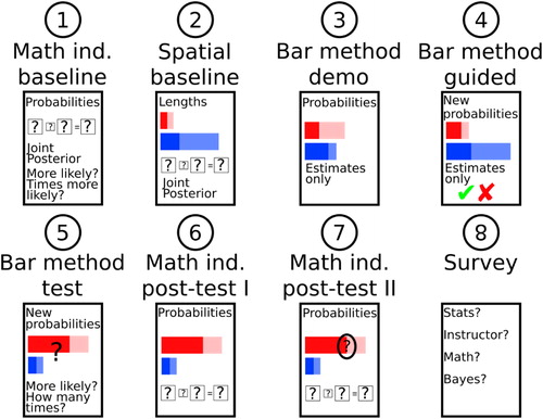
The first worksheet (“Math ind. baseline,” where ind. stand for induction) presented a probability-format Bayesian reasoning problem with the same “music reading” scenario used in Exercise 1. Participants were asked to specify (1) the math needed to find the proportion of students in the class who both know how to read music and own an instrument, (2) the math needed to find the proportion of students in the class who don’t know how to read music but do own an instrument, (3) whether a student in the class who owned an instrument was more likely to know how to read music or not, and (4) the math needed answer the question, “How many times more likely is the option you selected on question 3 than the other option?” As in Exercise 1, there were large boxes to indicate where the participant should fill in numbers and small boxes to indicate where they should fill in math operations. After the participant recorded their responses, the instructor collected the response sheet without providing feedback of any sort. As before, we will refer to the first two questions as the “multiplication rule” questions and score this component as correct if the participant correctly multiplies the appropriate conditional and marginal probabilities for both questions, and we will refer to the last two questions as the “posterior odds” question and score this component as correct if the participant correctly selects the more likely hypothesis and divides the joint probabilities that they calculated above to answer “How many times more likely?”

The second worksheet (“Spatial baseline”) introduced a new problem that described a carpenter cutting two planks of wood to a proportion of their original length to complete a construction project. The goal was to measure the participant’s ability to link spatial representations to math equations outside the context of a probability question. The problem was presented numerically to participants in a fashion analogous to the first worksheet, with numbers provided for the original length of each plank and the proportion of each plank that remained after they were cut. Participants also saw a bar display that represented the problem visually. The instructor read through the problem and briefly described how the content of the problem was represented on the visualization, describing only the basic components of the bar display such as the axis labels and legend. The participants were given no instructions on how to utilize the bar display to answer any of the worksheet’s questions but were encouraged to use the display as a tool to assist in their answering. After the instructions from the instructor, participants answered four questions that were analogous to those on the first worksheet. Once complete, the worksheet was set aside, and participants were given no feedback on whether their answers were correct.

Beginning with the third worksheet (“Bar method demo”), the participants learned how to construct and use the bar display. The participants were shown a worksheet that presented the same Bayesian reasoning problem from the first worksheet and were told that the instructor would draw a bar display to represent the information visually. For their role in the drawing, the participants were asked to follow along as the instructor created the bar display by hand and were encouraged to ask questions at any point during the instructions. The instructor identified each component of the Bayesian reasoning problem as he drew the bars and emphasized that all of the information given in the problem was explicitly highlighted in the visualization itself. Once the bar display was complete, the instructor demonstrated how each of the four questions from the first worksheet could be answered through estimations obtained from the visual. For example, the joint probability could be estimated by examining the length of the shaded region of each bar relative to the x-axis, and the posterior odds could be estimated by assessing spatially how many times longer one shaded region was compared to the other. Participants received no instruction on how to solve the problem with equations.

The fourth worksheet (“Bar method guided”) was again instructional and followed a format similar to the previous sheet, except that participants were tasked with verbally explaining how estimations for each of the four questions could be achieved using the bar display. For this worksheet, a new Bayesian reasoning problem was introduced and a bar display representing the new problem was created by the instructor. The instructor then read aloud each of the four questions and asked the participants to verbally explain how to approximately answer each question using the display. The participants were encouraged to fully explain their answers and to physically point to parts of the bar display that they were using to obtain each answer. The purpose of such verbalization was to test the participant’s understanding of the bar display and to provide an opportunity for additional clarification if the participants were struggling to understand components of the display. Again, no indication was given as to how each answer could be obtained mathematically.

Following instruction, the participant completed a new Bayesian reasoning problem in a two-worksheet sequence. First, they worked the problem on their own using the spatial method (“Bar method test”). This worksheet presented the problem text and asked participants to draw a bar display representing the problem. The instructor checked the display to ensure that it matched the problem information (all participants drew the display correctly without further guidance). After drawing the display, participants were asked to report the joint probabilities and posterior odds with the same four-question sequence as the “Bar method demo” and “Bar method guided” worksheets. No feedback was provided on their responses. When they finished, they were given the math-induction worksheet with the same problem text as the last worksheet (“Math ind. post-test I”). The instructor explained to the participant that they were going to work the same problem again, but this time they were going to attempt to solve it with equations instead of the spatial method. This post-training math induction sheet had the same questions and response options as the baseline math induction sheet (but not the same numbers in the problem). The instructor also gave the participant a sheet displaying a computer-generated figure of the correct bar display to use as a reference.

The final worksheet (“Math ind. post-test II”) provided a second chance to answer the math induction questions and was only administered to participants who responded incorrectly on Math ind. post-test I. This worksheet was identical to the previous one, except that the bar display was labeled to show which aspect of the display mapped to each math induction question. The participants were asked to double-check that their answers corresponded appropriately to the bar display. Each question was given a letter identification that corresponded to the labels on the bar display. In this way, the participants were prompted to remember how to estimate answers using the bar display and encouraged to use those estimations to reevaluate their mathematical answers.

We used two versions of the task, where Version B was created by taking Version A and switching the problem used before training on the “Math ind. baseline” and “Bar method guided” worksheets with the problem used after training on the “Bar method test” and “Math ind. post-test” worksheets. We alternated versions across subjects, and ended up with 15 and 14 participants run with Versions A and B, respectively.

4.2 Results

Our primary interest was the math induction success rates before and after training (from “Math ind. baseline” to “Math ind. post-test I” on Figure 5). Generally, success rates were pretty high even before training and increased after participants learned the spatial task. Specifically, success rates for correctly answering all components of the math induction sheet went from 41% to 69%, success rates for correctly answering both of the multiplication rule questions went from 59% to 76%, and success rates for correctly answering the posterior odds question went from 55% to 86%.

We used a multinomial model to estimate the proportion of students in the overall population who will succeed (“S”) and fail (“F”) on the math induction task before and after spatial training, creating four mutually exclusive categories (F-F, F-S, S-F, S-S). We used a Dirichlet distribution to define uncertainty in the multinomial parameters for the proportion of participants in each of the four categories, and we set all shape parameters to 1 for the prior distribution. Thus, our posterior distributions reflect only information from our sample. We combined the S-F and S-S categories to estimate success rates before training and the F-S and S-S categories to define success rates after training.

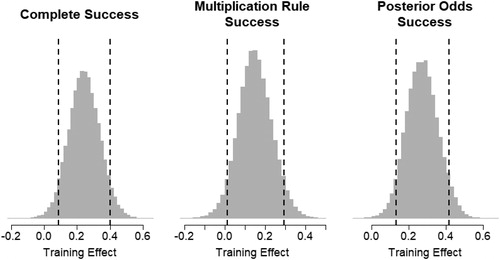
Figure 6 shows posterior distributions for the training effect (post-training minus pre-training success rates) where success is defined either by answering all of the math induction questions, by answering just the multiplication-rule questions, or by answering just the posterior-odds question. In all cases, the lower limit of the credible interval is above zero, indicating a high probability (over 95%) of positive training effects at the population level. Point estimates for the training effect indicated a meaningful effect size, and suggested that learning the spatial technique increases student success rates by 24 percentage points for the “complete success” measure, 15 percentage points for the multiplication rule questions, and 27 percentage points for the posterior odds question.

Fig. 6 Posterior distributions for the effect of spatial training; that is, the difference in success rates between pre- and post-training math induction tasks. The three histograms show three different criteria for success: answering all of the math induction questions correctly, answering the two multiplication rule questions correctly, and answering the posterior odds question correctly. The dashed vertical lines show 90% credible intervals.

As described in the procedure, we gave participants who erred on the math induction post-test a second chance with two added advantages: (1) a spatial display that more clearly linked elements of the display to the math induction problems, and (2) instructions to make sure that their math-derived answers match what they see on the spatial display (Math ind. post-test II in Figure 5). We did not see evidence that this additional prompting is a substantial help for the students who initially failed the math induction exercise. In fact, there was only one participant who recovered after an initial incorrect response for the multiplication rule questions and only one (separate) participant who recovered after an initial incorrect response for the posterior odds question.

Exercise 2 included a problem that participants were asked to solve using the spatial method without help from the instructor (spatial test in Figure 5). To assess how well they learned the spatial method, we scored whether they drew a bar display that correctly represented the problem information, whether they accurately estimated both joint probabilities (to within 0.05 of the true values), and whether they accurately estimated the posterior odds (to within 1 of the true value).² Results showed that participants were very successful in learning to use the spatial method. Every participant drew the bars in a way that accurately represented the problem information. We also observed a 100% success rate for estimating the value of both joint probabilities from the display. For the posterior odds, 93% of participants (all but 2) made accurate estimates.

The plank-task results showed that, before the spatial training, about half of the participants were able to map spatial relationships to math equations. We observed that 51% of participants answered all of the questions correctly, 62% were able to calculate the length of the remaining portion of both planks, and 62% were able to figure out that they needed to divide to figure out how many times longer one remaining portion was than the other.

Four participants who were scored as incorrect on the multiplication rule question subtracted the unfilled portion of each bar from the total length of the bar to get the correct values for the joint probabilities. Thus, the response was technically correct, but we scored it as incorrect because the unfilled portion of the bars was not given as a number in the problem, meaning that they relied on the visualization, and not an equation, to get part of their answer. It is possible that some or all of these participants would have applied the multiplication rule if we had clarified that they cannot use any numbers that they estimated from the display, but instead could only use numbers reported in the problem or calculated in a previous step.

The key finding from Exercise 2 is that our revised procedures succeeded in increasing post-training success rates for the posterior odds portion of the math induction task. Indeed, Exercise 2 produced higher success rates for all aspects of the task, and the results suggest that a strong majority of students can succeed in actively discovering the mathematical principles of Bayes’ theorem and related probability concepts. We also saw a clear increase in success rates from before to after spatial training on all aspects of the math induction task.

5 Discussion

We explored ways that a spatial technique for solving Bayesian inference problems could be used to teach probability concepts. We showed that elements of the spatial display have a one-to-one mapping to important equations underlying probabilistic reasoning, and we suggested that educators could use the parallel representations to promote active learning by challenging students to discover these equations after learning a spatial method for approximating the desired quantities. To explore the viability of this suggestion, we ran two tutoring exercises to estimate the proportion of students who can succeed in the active learning exercise.

One aspect of the math-induction task involved discovering the multiplication rule for finding the joint probability that a hypothesis is true and an observation is made. The participants practiced approximating this quantity by creating one bar that represented the marginal or prior probability of the hypothesis, P(H), and filling in this bar proportional to the conditional probability of the observation given the hypothesis, P(O$|$H), and we tested their ability to translate this spatial method into explicit equations. Success rates for correctly applying the multiplication rule were over 70% in both exercises. Thus, we have strong evidence that the majority of students are capable of discovering this mathematical principle after learning an analogous spatial method. Moreover, success rates were just under 60% even before the visual training in the Exercise 2 math induction baseline, which is further encouragement for an active learning approach to teaching this concept. Finally, our results supported a strong inference that multiplication rule performance increased after the spatial training even though it started from a fairly high baseline, so teachers can expect that using the spatial representation will help more of their students succeed in actively discovering the multiplication rule.

The fairly high success rate that the we observed for baseline multiplication rule performance contrasts with the low untrained performance on Bayesian inference problems, which is generally around 4% (McDowell and Jacobs 2017) and was 14% in our Exercise 1. This suggests that untrained students can achieve much higher success rates when asked to apply isolated components of Bayesian inference compared to when they are asked to combine components without guidance on individual steps.

Another aspect of the math-induction task involved finding the posterior odds that a hypothesis is true given an observation—that is, dividing the joint probability that the hypothesis is true and the observation is made by the joint probability that the hypothesis is false and the observation is made. Students learned to approximate this value by comparing the lengths of the filled portions of the two bars in the spatial display, and then they were challenged to specify an equation that corresponded to this spatial comparison. We observed that 59% of students succeeded in this active learning task in Exercise 1, and we designed Exercise 2 to try to improve success rates by showing students the step-by-step process of creating the bar display and by emphasizing the process of estimating posterior odds. These changes appeared to be successful, as we observed a success rate of 86% after spatial training in Exercise 2.

Overall, our results demonstrate that spatially-guided active-learning exercises will be successful for many students. This is significant for educators, because self-generated information is remembered substantially better than passively received information (Slamecka and Graf 1978) and students report preferring active-learning exercises over standard lecturing (Freeman et al. 2014). Moreover, all students will learn an independent solution method that the instructor can use to provide insight into the structure of the equations as learning progresses. In Exercise 2, we tested participants’ ability to implement the spatial technique on their own after a brief instruction phase in which the instructor demonstrated the technique for two other problems. The vast majority of participants (93%) correctly applied the technique to estimate both the joint probabilities and the posterior odds for a Bayesian inference problem, demonstrating that instruction with spatial representations has tangible benefits even for students who do not succeed in translating them into explicit equations.

Exercise 2 produced higher math induction success rates, so we recommend that educators emulate the Exercise 2 procedure when designing active-learning exercises. Specifically, we recommend that educators allow students to see the steps involved in creating the spatial display with a clear description of what each new element of the display represents. This could be achieved by drawing the display on the board or with staged slides showing a computer-generated display with a new component appearing on each new slide. For practice problems, we also recommend getting explicit confirmation from students about what components of the display they are using and why. This would ideally be an explicit part of answering the problem, for example, “Circle the part of the bar display you used to estimate the proportion of students in the class who both know how to read music and own an instrument.”

5.1 Math-Induction Mechanisms

The current exercises were designed to test whether an active learning approach is viable for educators, not to explore the theoretical processes involved in our math-induction task. Our results suggest that many students will succeed in active learning supported by spatial representations, but future investigations are needed to explore how the spatial training promotes success in math induction. Some of the underlying processes might be fairly prosaic, and might not rely on the spatial nature of our solution method. In this section, we discuss two of these general factors.

Linking the spatial display to explicit mathematics involves breaking the Bayes’ theorem equation into steps that correspond to identifiable elements of the display. Exercise 2 suggests that this “road map” to finding a solution is beneficial in itself. With the problem broken down into steps, 41% of participants were able to specify the correct math for all steps even before they learned the spatial method. This number is well above the expected rate of solving probability-format Bayesian reasoning problems for untrained participants, which is typically below 10% (McDowell and Jacobs 2017) and was 14% for the probability-baseline problem in our Exercise 1. Although our Exercise 2 baseline performance was impressively high for untrained participants, training in the spatial method substantially increased success rates, with 69% of participants able to specify the correct math for all steps by the end of the session. So the results strongly suggest that the spatial training is useful for helping students gain insight into the mathematical principles of Bayes’ theorem and related probability concepts. Also, the spatial display provides a way to show students why those steps are part of finding a solution, helping them understand how the step-by-step procedure relates to the larger goal of inferring what is likely to be true based on probabilistic information.

Our active learning procedure also gives students a chance to work through problems and get approximate answers without having to learn equations. This opportunity to solve practice problems could play a role in the observed success on the math-induction task. Past results suggest that college students are unlikely to figure out how to solve Bayesian reasoning problems just from repeated practice, even when they complete dozens of problems and receive feedback on the correct answer after each problem (e.g., Starns et al. 2018). However, it is possible that direct experience with example problems is more beneficial for our math-induction task because it isolates individual steps in the solution process. The role of general practice effects is an interesting topic for future theoretical experiments. For now, we note that attributing performance gains to practice effects would not detract from the value of the spatial method as an instructional tool. Indeed, one of the key benefits of the method is that is gives students a quick, intuitive way to perform approximate probabilistic reasoning before they are confronted with equations, so it provides a meaningful way for them to practice applying probability concepts. We doubt that students would respond positively to being confronted with multiple practice problems without knowing any method for answering them. The spatial method gives students a way to work practice problems without denying them the opportunity to independently discover the necessary equations as an active learning exercise. We are not aware of any other method that gives students a way to solve probability problems without teaching them any explicit equations, but if such methods are developed it will be interesting to compare them to the spatial method.

In summary, we acknowledge that factors like breaking the solution procedure into meaningful steps and experiencing practice problems are not uniquely tied to the spatial method, but the method provides a way to harness these benefits while also illustrating concepts in a format that some students might find more intuitive. Our results demonstrate that the method is a promising tool for educators, and this is true regardless of which specific underlying mechanisms support performance on the math-induction task.

5.2 Future Directions

5.2.1 Classroom Applications

The spatial method discussed here could be expanded in many ways in future research and application. One important question is how the spatial method compares to alternative teaching approaches in the classroom, both in terms of students’ initial learning experiences and the durability of their learning. We are beginning to address this question with a multiple-year classroom study. Another important question is whether students who fail to discover the correct math after learning the spatial technique could succeed with another active learning strategy. An optimal curriculum will likely need to incorporate a number of different ways to represent the same concept and explain the logic of solution procedures. The current results show that spatial methods are a useful element of this toolkit. Yet another future goal is to explore how spatial representations can help students understand more complex applications of Bayesian inference, such as parameter estimation.

Our goal was to estimate the proportion of students who are able to transfer a spatial solution method into explicit equations when working independently, and as a result, we also had students who received individual instruction on the spatial method. Using individual instruction potentially limits the external validity of the current results, as group instruction is more common in classrooms. Although we acknowledge the need for more exploration of our active learning approach in a group setting, Starns et al. (2018) reported one example of successful classroom-based application. When Starns et al. is considered together with the current results, we have evidence that our techniques can work in real classrooms as a group assignment and evidence that a high proportion of students can discover the equations independently. As such, we would expect to find high rates of success with group instruction followed by individual work on the math induction task, and we will explore this in future studies. In addition to further classroom work, another potential future direction is to develop a computerized “virtual tutor” system that students complete independently as a homework assignment, ideally one that adapts to the needs of individual students by tracking their accuracy at each step of the active-learning process.

An important goal for future research is exploring how the spatial method interacts with student characteristics. Unlike alternative visual displays, such as contingency tables and tree diagrams, the bars represent information both numerically and spatially. This dual representation could be especially beneficial for students who struggle with math or have negative attitudes about math, potentially helping a more diverse range of students succeed in fields with heavy statistical requirements.

5.2.2 Frequency Versus Probability

Past research shows that untrained participants are more likely to solve Bayesian inference problems in a nested-frequency format than a probability format (Gigerenzer and Hoffrage 1995; McDowell and Jacobs 2017). We replicated this pattern in Exercise 1, with participants achieving solution rates of 45% and 14% for the untrained frequency- and probability-format problems, respectively. Our primary goal is helping students understand probability and statistical reasoning, so we have focused on whether participants can discover the math for probability-format problems. Generally, statistics instructors will also want their students to be able to work directly with probabilities, of course. That said, linking the nested-frequency and probability formats might enhance the success of an active learning approach by capitalizing on peoples’ keener intuition for the nested-frequency format. Starns et al. (2018) showed how the bar display could be used to translate between frequency and probability formats by demonstrating to students that the spatial relationships of the display components are exactly the same for the two formats. Future studies can evaluate whether spatial representations help students recognize the shared features of frequency and probability formats.

5.3 Conclusion

Probabilistic reasoning is a fundamental skill for many STEM fields and the backbone of statistical inference. Given the well-documented learning benefits of self-generation (Slamecka and Graf 1978) and the educational benefits of promoting active learning (Freeman et al. 2014), we have attempted to develop techniques that allow students to independently discover the equations associated with important probability concepts by analogy to a spatial solution method. Our results suggest that the majority of students can specify the mathematical steps required to find a joint probability, calculate an odds value, and apply Bayes’ theorem after learning a spatial method for approximating the solution to probability problems.

Acknowledgments

We thank Joseph Vazquez for helping us collect data in Experiment 2.

Data Availability Statement

Files are available on the OSF at this link: https://osf.io/aq7w3/?view_only=ccb6dc5b367e419facc7965b3a0caaf5. The available files include data-scoring files, scanned response sheets of the session activities, and audio recordings of the session for participants who consented to recording.

Disclosure Statement

No potential conflict of interest was reported by the author(s).

Additional information

Funding

Research activities were supported by NSF grant DUE-1842537 awarded to authors JJS and ALC.

Notes

1 We did not test both posterior odds and posterior probability in the exercises below because they provide redundant information; an odds value can be transformed to a probability and vice versa. We focus on odds instead of probability because the former is more directly observable in the spatial display.

2 We used each participant’s estimates of the joint probabilities to define the correct posterior odds. We did this to accommodate variation in how participants drew the spatial display, with the rationale that their own responses carry the best information about what they are seeing on the display they created.

References

- Bar-Hillel, M. (1980), “The Base-Rate Fallacy in Probability Judgments,” Acta Psychologica, 44, 211–233. DOI: 10.1016/0001-6918(80)90046-3.
- Binder, K., Krauss, S., and Bruckmaier, G. (2015), “Effects of Visualizing Statistical Information—An Empirical Study on Tree Diagrams and 2 × 2 Tables,” Frontiers in Psychology, 6, 1186.
- Böcherer-Linder, K., and Eichler, A. (2017), “The Impact of Visualizing Nested Sets. An Empirical Study on Tree Diagrams and Unit Squares,” Frontiers in Psychology, 7, 2026. DOI: 10.3389/fpsyg.2016.02026.
- Böcherer-Linder, K., and Eichler, A. (2019), “How to Improve Performance in Bayesian Inference Tasks: A Comparison of Five Visualizations,” Frontiers in Psychology, 10, 267.
- Brase, G. L. (2009), “Pictorial Representations in Statistical Reasoning,” Applied Cognitive Psychology, 23, 369–381. DOI: 10.1002/acp.1460.
- Brase, G. L. (2014), “The Power of Representation and Interpretation: Doubling Statistical Reasoning Performance With Icons and Frequentist Interpretations of Ambiguous Numbers,” Journal of Cognitive Psychology, 26, 81–97.
- Cohen, A. L., Sidlowski, S., and Staub, A. (2017), “Beliefs and Bayesian Reasoning,” Psychonomic Bulletin & Review, 24, 972–978.
- Cohen, A. L., and Staub, A. (2015), “Within-Subject Consistency and Between-Subject Variability in Bayesian Reasoning Strategies,” Cognitive Psychology, 81, 26–47. DOI: 10.1016/j.cogpsych.2015.08.001.
- Cosmides, L., and Tooby, J. (1996), “Are Humans Good Intuitive Statisticians After All? Rethinking Some Conclusions From the Literature on Judgment Under Uncertainty,” Cognition, 58, 1–73. DOI: 10.1016/0010-0277(95)00664-8.
- Diaconis, P., and Freedman, D. (1981), “The Persistence of Cognitive Illusions,” The Behavioral and Brain Sciences, 4, 333–334. DOI: 10.1017/S0140525X00009122.
- Freeman, S., Eddy, S. L., McDonough, M., Smith, M. K., Okoroafor, N., Jordt, H., and Wenderof, M. P. (2014), “Active Learning Increases Student Performance in Science, Engineering, and Mathematics,” Proceedings of the National Academy of Sciences of the United States of America, 111, 8410–8415. DOI: 10.1073/pnas.1319030111.
- Gigerenzer, G., and Hoffrage, U. (1995), “How to Improve Bayesian Reasoning Without Instruction: Frequency Formats,” Psychological Review, 102, 684–704. DOI: 10.1037/0033-295X.102.4.684.
- Givven, K. B., Moroz, V., Loftus, W., and Stigler, J. W. (2019), “Removing Opportunities to Calculate Improves Students’ Performance on Subsequent Word Problems,” Cognitive Research: Principles and Implications, 4, 24. DOI: 10.1186/s41235-019-0175-2.
- Koski, T., and Noble, J. M. (2009), Bayesian Networks: An Introduction, West Sussex, UK: Wiley.
- Kruschke, J. K. (2011), Doing Bayesian Data Analysis: A Tutorial With R and BUGS, Burlington, MA: Academic Press.
- Kurzenhäuser, S., and Hoffrage, U. (2002), “Teaching Bayesian Reasoning: An Evaluation of a Classroom Tutorial for Medical Students,” Medical Teacher, 24, 516–521. DOI: 10.1080/0142159021000012540.
- Martinez, E. Z., and Achar, J. A. (2014), “Trends in Epidemiology in the 21st Century: Time to Adopt Bayesian Methods,” Methodological Issues, 30, 703–714. DOI: 10.1590/0102-311x00144013.
- McDowell, M. and Jacobs, P. (2017), “Meta-Analysis of the Effect of Natural Frequencies on Bayesian Reasoning,” Psychological Bulletin, 143, 1273–1312. DOI: 10.1037/bul0000126.
- Micallef, L., Dragicevic, P., and Fekete, J. (2012), “Assessing the Effect of Visualizations on Bayesian Reasoning Through Crowdsourcing,” IEEE Transactions on Visualization and Computer Graphics, 18, 2536–2545. DOI: 10.1109/TVCG.2012.199.
- Reani, M., Davies, A., Peek, N., and Jay, C. (2018), “How Do People Use Information Presentation to Make Decisions in Bayesian Reasoning Tasks?,” International Journal of Human-Computer Studies, 111, 62–77. DOI: 10.1016/j.ijhcs.2017.11.004.
- Satake, E., and Vashlishan Murray, A. (2015), “An Alternative Teaching Method of Conditional Probabilities and Bayes’ Rule: An Application of the Truth Table,” Teaching Statistics, 37, 89–95. DOI: 10.1111/test.12080.
- Sedlmeier, P., and Gigerenzer, G. (2001), “Teaching Bayesian Reasoning in Less Than Two Hours,” Journal of Experimental Psychology: General, 130, 380–400. DOI: 10.1037/0096-3445.130.3.380.
- Sirota, M., Kostovièová, L., and Juanchich, M. (2014), “The Effect of Iconicity of Visual Displays on Statistical Reasoning: Evidence in Favor of the Null Hypothesis,” Psychonomic Bulletin & Review, 21, 961–968.
- Slamecka, N. J., and Graf, P. (1978), “The Generation Effect: Delineation of a Phenomenon,” Journal of Experimental Psychology: Human Learning and Memory, 4, 592–604.
- Sloman, S. A., Over, D., Slovak, L., and Stibel, J. M. (2003), “Frequency Illusions and Other Fallacies,” Organizational Behavior and Human Decision Processes, 91, 296–309. DOI: 10.1016/S0749-5978(03)00021-9.
- Starns, J. J., Cohen, A. L., Bosco, C., and Hirst, J. (2018), “A Visualization Technique for Bayesian Reasoning,” Applied Cognitive Psychology, 33, 234–251. DOI: 10.1002/acp.3470.
- Thompson, W. C., and Shumann, E. L. (1987), “Interpretation of Statistical Evidence in Criminal Trials: The Prosecutor’s Fallacy and the Defense Attorney’s Fallacy,” Law and Human Behavior, 2, 167–187. DOI: 10.1007/BF01044641.
- Tversky, A., and Kahneman, D. (1983), “Extensional Versus Intuitive Reasoning: The Conjunction Fallacy in Probability Judgment,” Psychological Review, 90, 293–315. DOI: 10.1037/0033-295X.90.4.293.
- Wiggins, G. (1998), Educative Assessment, San Francisco, CA: Jossey-Bass.
- Wu, C. M., Meder, B., Filimon, F., and Nelson, J. D. (2017), “Asking Better Questions: How Presentation Formats Influence Information Search,” Journal of Experimental Psychology: Learning, Memory, and Cognition, 43, 1274–1297.
- Yamagishi, K. (2003), “Facilitating Normative Judgments of Conditional Probability: Frequency or Nested Sets?,” Experimental Psychology, 50, 97–106. DOI: 10.1026//1618-3169.50.2.97.