Mixture Simultaneous Factor Analysis for Capturing Differences in Latent Variables Between Higher Level Units of Multilevel Data

Abstract

Given multivariate data, many research questions pertain to the covariance structure: whether and how the variables (e.g., personality measures) covary. Exploratory factor analysis (EFA) is often used to look for latent variables that might explain the covariances among variables; for example, the Big Five personality structure. In the case of multilevel data, one might wonder whether or not the same covariance (factor) structure holds for each so-called data block (containing data of 1 higher level unit). For instance, is the Big Five personality structure found in each country or do cross-cultural differences exist? The well-known multigroup EFA framework falls short in answering such questions, especially for numerous groups or blocks. We introduce mixture simultaneous factor analysis (MSFA), performing a mixture model clustering of data blocks, based on their factor structure. A simulation study shows excellent results with respect to parameter recovery and an empirical example is included to illustrate the value of MSFA.

Keywords:

• factor analysis
• latent variables
• mixture model clustering
• multilevel data

Given multivariate data, researchers often wonder whether the variables covary to some extent and in what way. For instance, in personality psychology, there has been a debate about the structure of personality measures (i.e., the Big Five vs. Big Three debate; De Raad et al., 2010). Similarly, emotion psychologists have discussed intensely whether and how emotions as well as norms for experiencing emotions can be meaningfully organized in a low-dimensional space (e.g., Ekman, 1999; Fontaine, Scherer, Roesch, & Ellsworth, 2007; Russell & Barrett, 1999; Stearns, 1994). Factor analysis (Lawley & Maxwell, 1962) is an important tool in these debates as it explains the covariance structure of the variables by means of a few latent variables, called factors. When the researchers have a priori assumptions on the number and nature of the underlying latent variables, confirmatory factor analysis (CFA) is often used, whereas exploratory factor analysis (EFA) is applied when one has no such assumptions.

Research questions about the covariance structure get further ramifications when the data have a multilevel structure; for instance, when personality measures are available for inhabitants from different countries. We refer to data organized according to the higher level units (e.g., the countries) as data blocks. For multilevel data, one can wonder whether or not the same structure holds for each data block. For example, is the Big Five personality structure found in each country or not (De Raad et al., 2010)? Similarly, many cross-cultural psychologists argue that the structure of emotions and emotion norms differ between cultures (Eid & Diener, 2001; Fontaine, Poortinga, Setiadi, & Markam, 2002; MacKinnon & Keating, 1989; Rodriguez & Church, 2003).

When looking for differences and similarities in covariance structures, using EFA is very advantageous because it leaves more room for finding differences than CFA does. For instance, in the emotion norm example (Eid & Diener, 2001), one might very well expect two latent variables to show up in each country corresponding to approved and disapproved emotions, being clueless about which emotions will be (dis)approved and how this differs across countries. In the search for such differences and similarities, one might perform a multigroup or multilevel¹ EFA (Dolan, Oort, Stoel, & Wicherts, 2009; Hessen, Dolan, & Wicherts, 2006; Muthén, 1991), or an EFA per data block. These methods fall short in answering the research question at hand, however. Multigroup or multilevel EFA can be used to test whether or not between-group differences in factors are present, but neither of them indicate how they are different and for which data blocks. When multigroup or multilevel EFA indicates the presence of between-block differences, one can compare the block-specific EFA models to pinpoint differences and similarities. When many groups are involved, however, the numerous pairwise comparisons are neither practical nor insightful; that is, it is hard to draw overall conclusions based on a multitude of pairwise similarities and dissimilarities. For instance, we present data on emotion norms for 48 countries. Because multigroup EFA indicates that the factor structure is not equal across groups, comparing the group-specific structures would be the next step. It would be a daunting task, however, with no fewer than 1,128 pairwise comparisons. More important, subgroups of data blocks might exist that share essentially the same structure and finding these subgroups is substantively interesting. Multilevel mixture factor analysis (MLMFA; Varriale & Vermunt, 2012) performs a mixture clustering of the data blocks based on some parameters of their underlying factor model, but it does not allow the factors themselves to differ across the data blocks.

Within the deterministic modeling framework, however, a method exists that clusters data blocks based on their underlying covariance structure and performs a simultaneous component analysis (SCA, which is a multigroup extension of standard principal component analysis [PCA]; Timmerman & Kiers, 2003) per cluster. The so-called clusterwise SCA (De Roover, Ceulemans, & Timmerman, 2012; De Roover, Ceulemans, Timmerman, Nezlek, & Onghena, 2013; De Roover, Ceulemans, Timmerman, & Onghena, 2013; De Roover, Ceulemans, Timmerman, et al., 2012) has proven its merit in answering questions pertaining to differences and similarities in covariance structures (Brose, De Roover, Ceulemans, & Kuppens, 2015; Krysinska et al., 2014). However, the method also has an important drawback, which follows from its deterministic nature, in that no inferential tools are provided for examining parameter uncertainty (e.g., standard errors, confidence intervals), conducting hypothesis tests (e.g., to determine which factor loading differences between clusters are significant), and performing model selection. Furthermore, even though similarities between component and factor analyses have been well-documented (Ogasawara, 2000; Velicer & Jackson, 1990; Velicer, Peacock, & Jackson, 1982), the theoretical status of components and factors is not the same (Borsboom, Mellenbergh, & van Heerden, 2003; Gorsuch, 1990). Therefore, to examine covariance structure differences in terms of differences in underlying latent variables (i.e., unobservable variables that have a causal relationship to the observed variables), such as the previously mentioned personality traits and affect dimensions, an EFA-based method is to be preferred.

Therefore, we introduce mixture simultaneous factor analysis (MSFA), which encompasses a mixture model clustering of the data blocks, based on their underlying factor structure. MSFA can be estimated by means of Latent GOLD (LG; Vermunt & Magidson, 2013) or Mplus (Muthén & Muthén, 2005). Even though the stochastic framework provides many inferential tools, various adaptations of the software will be necessary to reach the full inferential potential of the MSFA method (i.e., for the tools to be applicable for MSFA, as explained later). Therefore, this article focuses mainly on the model specification and an extensive evaluation of the goodness-of-recovery; that is, how well MSFA recovers the clustering as well as the cluster-specific factor models.

The remainder of this article is organized as follows. In the next section, the multilevel multivariate data structure and its preprocessing is discussed, as well as the model specifications of MSFA, followed by its model estimation and its relations to existing mixture or multilevel factor analysis methods. The performance of MSFA is then evaluated in an extensive simulation study, followed by an illustration of the method with an application. Finally, the paper concludes with points of discussion and directions for future research.

MIXTURE SIMULTANEOUS FACTOR ANALYSIS

Data Structure and Preprocessing

We assume multilevel data, which implies that observations or lower level units are nested within higher level units (e.g., patients within hospitals, pupils within schools, inhabitants within countries). Both the lower and the higher level units are assumed to be a random sample of the population of lower and higher level units, respectively. We index the higher level units by i = 1, …, I and the lower level units by n_i = 1, …, N_i. The data of each higher-level unit i is gathered in an N_i × J data matrix or data block X_i, where J denotes the number of variables. Because MSFA focuses on modeling the covariance structure of the data blocks (within-block structure; Muthén, 1991), irrespective of differences and similarities in their mean level (between-block structure), all data blocks are columnwise centered before the analysis.

Model Specification

MSFA applies common factor analysis at the observation level and a mixture model at the level of the data blocks. Specifically, we assume (a) that the observations are sampled from a mixture of normal distributions that differ with respect to their covariance matrices, but all have a zero mean vector (which corresponds to all data blocks being columnwise centered beforehand² ), and (b) that all observations of a data block are sampled from the same normal distribution.

More formally, the MSFA model can be written as follows:

(1)

where f is the total population density function, and θ refers to the total set of parameters. Similarly, f_k refers to the kth cluster-specific density function and θ_k refers to the corresponding set of parameters. The latter densities are specified as K normal distributions, the covariance matrices of which are modeled by cluster-specific factor models. Thus, θ_k refers to the cluster-specific factor loadings in the J × Q matrix (implying the number of factors Q to be the same across clusters³ ) and the unique variances on the diagonal of . The mixing proportions (i.e., the prior probabilities of a data block belonging to each of the clusters) are indicated by , with . Equation 1 implies the following additional assumptions: First, the cluster-specific covariance matrices are perfectly modeled by the corresponding low-rank cluster-specific factor models (i.e., no residual covariances, implying that is a diagonal matrix). Second, within each block, the observations are locally independent, warranting the use of the multiplication operator in Equation 1. Third, we impose the factor scores and the residuals to be normally distributed for each data block, with the covariance matrix of the factor scores being an identity matrix and that of the residuals being equal to . In this article, the factor (co)variance matrix is restricted to equal identity for each data block to capture all differences in observed-variable covariances by means of the cluster-specific factor loadings—which implies creating the exact stochastic counterpart of the clusterwise SCA variant described by De Roover, Ceulemans, Timmerman, Vansteelandt, et al., (2012). This has the interpretational advantage of establishing all structural differences without having to inspect the (possibly many) block-specific factor (co)variances. Of course, more flexible model specifications in terms of the factor (co)variances are possible. Note that the cluster-specific factors have rotational freedom, which we take into account by using a rotational criterion, such as Varimax (Kaiser, 1958) and generalized Procrustes rotation (Kiers, 1997), that enhances the interpretability of the factor loading structures. Because factor rotation is not yet included in LG, we take the loadings estimated by LG 5.1 and rotate them in Matlab R2015b.

By means of Bayes’s theorem, the posterior classification probabilities of the data blocks can be calculated, giving information regarding the blocks’ cluster memberships and the uncertainty about this clustering. Specifically, these probabilities pertain to the posterior distribution (i.e., conditional on the observed data) of the latent cluster memberships z_ik:

(2)

Relations to Existing Methods

Because MSFA is an exploratory method, we omit related confirmatory methods like mixture factor analysis (Lubke & Muthén, 2005; Muthén, 1989; Yung, 1997), factor mixture analysis (Blafield, 1980; Yung, 1997), multilevel factor mixture modeling (Kim, Joo, Lee, Wang, & Stark, 2016), and a number of multigroup CFA extensions (Asparouhov & Muthén, 2014; Jöreskog, 1971; Muthén & Asparouhov, 2013; Sörbom, 1974). As mentioned earlier, methods based on CFA leave less room to find differences. Indeed, CFA imposes an assumed structure of zero loadings on the factors; thus, CFA-based methods can only account for differences in the size of the freely estimated (i.e., nonzero) factor loadings. Specifically, we compare MSFA to (a) a nonmultilevel mixture EFA model, called mixtures of factor analyzers (MoFA; McLachlan & Peel, 2000), and (b) a multilevel mixture EFA model, MLMFA (Varriale & Vermunt, 2012).

MoFA performs a mixture clustering of individual observations based on their underlying EFA model. The observation-level clusters differ with respect to their intercepts, factor loadings, and unique variances, whereas the factors have means of zero and an identity covariance matrix per cluster. In contrast, MSFA deals with block-centered multilevel data and clusters data blocks (instead of individual observations) based on their factor loadings and unique variances (omitting the intercepts).

MLMFA models between-block differences in intercepts, factor means, factor (co)variances, and unique variances by a mixture clustering of the data blocks, but MLMFA requires equal factor loadings across blocks. Hence, the MLMFA model specification differs in the following respects from MSFA. First, unlike in MSFA, the cluster-specific means of the K multivariate normal distributions are not restricted to zero and capture between-block differences in mean levels on either the observed variables (intercepts) or the latent variables (factor means). Second, unlike MSFA, MLMFA models differences in covariance structures by means of differences in unique variances and factor (co)variances but not by differences in factor loadings (i.e., in contrast to Equation 1, loadings are common across clusters). Thus the range of covariance differences that MLMFA can capture is rather limited when compared to MSFA. Moreover, because both mean levels and covariance structures are taken into account, the MLMFA clustering will often be dominated by the means because they have a larger influence on the fit, whereas with MSFA mean differences are discarded.

Model Estimation

The unknown parameters θ of the MSFA model are estimated by means of maximum likelihood (ML) estimation. This involves maximizing the logarithm of the likelihood function:

(3)

where X is the N × J data matrix—with —that is obtained by vertically concatenating the I data blocks X_i. Note that the likelihood function is computed as a product of the likelihood contributions of the I data blocks, assuming that they are a random sample and thus mutually independent. To find the parameter estimates that maximize Equation 3, ML estimation is performed by LG, which uses a combination of an expectation maximization (EM) algorithm and a Newton–Raphson algorithm (NR; see Appendix A). Because the standard random starting values procedure turned out to be rather prone to local maxima (especially when the number of clusters or factors increases), we experimented with alternative starting procedures. Appendix A describes the procedure we used, which involves starting with a PCA solution to which randomness is added.

SIMULATION STUDY

Problem

To evaluate the model estimation performance in terms of the sensitivity to local maxima and goodness of recovery, data sets were generated (by LG 5.1) from an MSFA model with a known number of clusters K and factors Q. We manipulated six factors that all affect cluster separation: (a) the between-cluster similarity of factor loadings, (b) the number of data blocks, (c) the number of observations per data block, (d) the number of underlying clusters and (e) factors, and (f) between-variable differences in unique variances. Factor 1 pertains to the similarity of the clusters and we anticipate the performance to be lower when clusters have more similar factor loadings. Factors 2 and 3 pertain to sample size. We expect the MSFA algorithm to perform better with increasing sample sizes (i.e., more data blocks or observations per data block; de Winter, Dodou, & Wieringa, 2009; Steinley & Brusco, 2011). With respect to Factors 4 and 5 (i.e., the complexity of the underlying model), we hypothesize that the performance will decrease with increasing complexity (de Winter et al., 2009; Steinley & Brusco, 2011). Factor 6, between-variable differences in unique variances, was manipulated to study whether and to what extent the performance of MSFA is affected by these differences. Theoretically, MSFA should be able to deal with these differences perfectly, in contrast to the existing clusterwise SCA, which makes no distinction between common and unique variances (De Roover, Ceulemans, Timmerman, Vansteelandt, et al. 2012).

Design and Procedure

The six factors were systematically varied in a complete factorial design:

1. The between-cluster similarity of factor loadings at two levels: medium, high similarity.

2. The number of data blocks I at three levels: 20, 100, 500.

3. The number of observations per data block N_i at five levels: for the sake of simplicity, N_i is chosen to be the same for all data blocks; specifically, equal to 5, 10, 20, 40, 80.

4. The number of clusters K at two levels: 2, 4.

5. The number of factors Q at two levels: 2, 4.

6. Between-variable differences in unique variances: Differences among the diagonal elements in D_k (k = 1, …, K) are either absent or present (explained later).

With respect to the cluster-specific factor loadings, a binary simple structure matrix was used as a common base for each . In this base matrix, the variables are equally divided over the factors; that is, each factor gets six loadings equal to one in the case of two factors, and three loadings equal to one in case of four factors (see Table 1). To obtain medium between-cluster similarity (Factor 1), each cluster-specific loading matrix was derived from this base matrix by shifting the high loading to another factor for two variables, whereas these variables differ among the clusters (see Table 1). For the high similarity level, each was constructed from the base matrix by adding, for each of two variables, a crossloading of √(.4) and lowering the primary loading accordingly (see Table 1). Note that the factor loadings are constructed such that each observed variable has the same common variance per cluster—that is, (1 – e_k), where e_k is the mean of the unique variances within a cluster. To quantify the similarity of the obtained cluster-specific factor loading matrices, they were orthogonally Procrustes rotated to each other (i.e., for each pair of matrices, one was chosen to be the target matrix and the other was rotated toward the target matrix) and a congruence coefficient (Tucker, 1951) was computed⁴ for each pair of corresponding factors in all pairs of matrices, where a congruence of one indicates that the two factors are proportionally identical. Subsequently, a grand mean of the obtained values was calculated, over the factors and cluster pairs. On average, amounted to .73 for the medium similarity condition and .93 for the high similarity condition.

TABLE 1 Base Loading Matrix and the Derived Cluster-Specific Loading Matrices for Clusters 1 and 2, in the Case of Two Factors (Top) and in the Case of Four Factors (Bottom)

	Base Loading Matrix				Cluster 1				Cluster 2
	Factor 1		Factor 2		Factor 1		Factor 2		Factor 1		Factor 2
Var. 1	1		0						1		0
Var. 2	1		0		1		0
Var. 3	1		0		1		0		1		0
Var. 4	1		0		1		0		1		0
Var. 5	1		0		1		0		1		0
Var. 6	1		0		1		0		1		0
Var. 7	0		1						0		1
Var. 8	0		1		0		1
Var. 9	0		1		0		1		0		1
Var. 10	0		1		0		1		0		1
Var. 11	0		1		0		1		0		1
Var. 12	0		1		0		1		0		1
	F1	F2	F3	F4	F1	F2	F3	F4	F1	F2	F3	F4
Var. 1	1	0	0	0			0	0	1	0	0	0
Var. 2	1	0	0	0	1	0	0	0			0	0
Var. 3	1	0	0	0	1	0	0	0	1	0	0	0
Var. 4	0	1	0	0			0	0	0	1	0	0
Var. 5	0	1	0	0	0	1	0	0			0	0
Var. 6	0	1	0	0	0	1	0	0	0	1	0	0
Var. 7	0	0	1	0	0	0	1	0	0	0	1	0
Var. 8	0	0	1	0	0	0	1	0	0	0	1	0
Var. 9	0	0	1	0	0	0	1	0	0	0	1	0
Var. 10	0	0	0	1	0	0	0	1	0	0	0	1
Var. 11	0	0	0	1	0	0	0	1	0	0	0	1
Var. 12	0	0	0	1	0	0	0	1	0	0	0	1

Note. In the case of medium similarity equals 0 and equals 1, whereas in the case of high similarity equals √(.6) and equals √(.4). When the number of clusters is four, the two additional loading matrices are constructed similarly; for example, in the four factor case, by shifting the primary loading or adding a cross-loading for Variables 3 and 6 for Cluster 3, and for Variables 4 and 7 for Cluster 4.

Regarding Factor 6, the first level of this factor was realized by simply setting each diagonal element of D_k equal to e_k. For the second level, differences in unique variance were introduced by ascribing a unique variance of (e_k − e_k/2) to a randomly chosen half of the variables and a unique variance of (e_k + e_k/2) to the other half of the variables.

The simulated data were generated as follows: The number of variables J was fixed at 12 and an overall unique variance ratio e of .40 was pursued for all simulated data sets, where . Between-cluster differences in e_k were introduced for all data sets, because they are usually present in empirical data sets. Specifically, in the case of two clusters, the e_k values are .20 and .60, whereas in the case of four clusters, the intermediate values of .30 and .50 are added for the additional clusters. To keep the overall variance equal across the clusters, the matrices were row-wise rescaled by . Finally, to make the simulation more challenging, the cluster sizes were made unequal. Specifically, the data blocks are divided over the clusters such that one cluster is three times smaller than the other cluster(s). Thus, in the case of two clusters, 25% of the data blocks were in one cluster and 75% in the other one. In the case of four clusters, the small cluster contained 10% of the data blocks whereas the other clusters consisted of 30% each. The cluster memberships were generated by randomly assigning the correct number of data blocks to each cluster, according to these cluster sizes.

For each cell of the factorial design, 20 raw data matrices were generated, using the LG simulation procedure, as described in Appendix C. The matrices resulting from the procedure were centered per variable, and their vertical concatenation yields the total data matrix X. In total, 2 (between-cluster similarity of factor loadings) × 3 (number of data blocks) × 5 (number of observations per data block) × 2 (number of clusters) × 2 (number of factors) × 2 (between-variable differences in unique variances) × 20 (replicates) = 4,800 simulated data matrices were generated. Each data matrix X was analyzed by means of an LG syntax specifying an MSFA model with the correct number of clusters K and factors Q (e.g., Appendix B) and applying 25 different sets of initial values (generated as described in Appendix A). No convergence problems were encountered in this simulation study.

Results

First, the sensitivity to local maxima is evaluated. Second, the goodness of recovery is discussed for the different aspects of the MSFA model: the clustering, the cluster-specific factor loadings, and the cluster-specific unique variances. Finally, some overall conclusions are drawn.

Sensitivity to local maxima

To evaluate the occurrence of local maximum solutions, we should compare the log L value of the best solution obtained by the multistart procedure with the global ML solution for each simulated data set. The global maximum is unknown, however, because the simulated data do not perfectly comply with the MSFA assumptions and contain error. Alternatively, we make use of a proxy of the global ML solution; that is, the solution that is obtained when the algorithm applies the true parameter values as starting values. The final solution from the multistart procedure is then considered to be a local maximum when its log L value is smaller than the one from the proxy. By this definition, only 227 (4.7%) local maxima were detected over all 4,800 simulated data sets. Not surprisingly, most of these occur in the more difficult conditions; for example, 179 of the 227 local maxima are found in the conditions with a high between-cluster similarity of the factor loadings and 153 are found for the most complex models; that is, when K as well as Q equal four.

Goodness of cluster recovery

To examine the goodness of recovery of the cluster memberships of the data blocks, we (a) compare the modal clustering (i.e., assigning each data block to the cluster for which the posterior probability is the highest) to the true clustering, and (b) investigate the degree of certainty of these classifications. To compare the modal clustering to the true one, the Adjusted Rand Index (ARI; Hubert & Arabie, 1985) is computed. The ARI equals 1 if the two partitions are identical, and equals 0 when the overlap between the two partitions is at chance level. The mean ARI over all data sets amounts to .93 (SD = 0.18), which indicates a good recovery. The ARI was affected most by the amount of available information. Specifically, the mean ARI for the conditions with only 20 data blocks and five observations per block was only .51, whereas the mean over the other conditions was .96.

To examine the classification certainty (CC), we computed the following statistics:

(4)

where and indicate the posterior probabilities (Equation 2) and the modal cluster memberships (i.e., estimates of the latent cluster membership z_ik), respectively. On average, CC_mean and CC_min amount to .9983 (SD = 0.007) and .94 (SD = 0.14), respectively, indicating a very high degree of certainty for the simulated data sets. Because CC_mean hardly varies over the simulated data sets, we focused on CC_min and inspected to what extent it is related to cluster recovery. To this end, a scatterplot of CC_min versus the ARI is given in Figure 1. From Figure 1, it is apparent that lack of classification certainty often does not coincide with classification error or the other way around.

FIGURE 1 Scatter plot of CC_min versus ARI for the simulated data sets.

Goodness of loading recovery

To evaluate the recovery of the cluster-specific loading matrices, we obtained a goodness-of-cluster-loading-recovery statistic (GOCL) by computing congruence coefficients (Tucker, 1951) between the loadings of the true and estimated factors and averaging across factors and clusters as follows:

(5)

with and indicating the true and estimated loading vector of the qth factor for cluster k, respectively. The rotational freedom of the factors per cluster was dealt with by an orthogonal Procrustes rotation of the estimated toward the true loading matrices. To account for the permutational freedom of the cluster labels, the permutation was chosen that maximizes the GOCL value. The GOCL statistic takes values between 0 (no recovery at all) and 1 (perfect recovery). For the simulation, the average GOCL is .98 (SD = 0.04), which corresponds to an excellent recovery. As for the clustering, the loading recovery depends strongly on the amount of information; that is, the mean GOCL is .87 for the conditions with only 20 data blocks and five observations per block and .99 for the remaining conditions.

Goodness of unique variance recovery

To quantify how well the cluster-specific unique variances are recovered, we calculated the mean absolute difference (MAD) between the true and estimated unique variances:

(6)

On average, the MAD_uniq was equal to .06 (SD = 0.06). Like the cluster and loading recovery, the unique variance recovery depends most on the amount of information; that is, the MAD_uniq has a mean value of .22 for the conditions with 20 data blocks or five observations per data block and .05 for the other conditions. Also, the MAD_uniq value is affected by the occurrence of Heywood cases (Van Driel, 1978), a common issue in factor analysis pertaining to “improper” factor solutions with at least one unique variance estimated as being negative or equal to zero. When this occurs during the estimation process, LG restricts it to be equal to a very small number (Vermunt & Magidson, 2013). Therefore, for the simulation, we consider a solution to be a Heywood case when at least one unique variance in one cluster is smaller than .0001. This was the case for 633 (13.2%) out of the 4,800 data sets, most of which occurred in the conditions with 20 blocks or five observations per block and thus with small within-cluster sample sizes (i.e., 601 out of the 633), or in the case of four factors per cluster (i.e., 522 out of the 633). Specifically, the mean MAD_uniq is equal to .18 for the Heywood cases and .04 for the other cases. In the literature, a Heywood case has been considered a diagnostic of problems such as (empirically) underdetermined factors or insufficient sample size (McDonald & Krane, 1979; Rindskopf, 1984; Van Driel, 1978; Velicer & Fava, 1998).

Conclusion

The low sensitivity to local maxima indicated that the applied multistart procedure is sufficient. The goodness-of-recovery for the clustering, and cluster-specific factor loadings and unique variances was very good, even in the case of very subtle between-cluster differences in loading pattern, and was mostly affected by the within-cluster sample size.

APPLICATION

To illustrate the empirical value of MSFA, we applied it to cross-cultural data on norms for experienced emotions from the International College Survey (ICS) 2001 (Diener, Kim-Prieto, & Scollon, 2001; Kuppens, Ceulemans, Timmerman, Diener, & Kim-Prieto, 2006). The ICS study included 10,018 participants from 48 different nations. Each of them rated, among other things, how much each of 13 emotions is appropriate, valued and approved in their society, using a 9-point Likert scale ranging from 1 (people do not approve it at all) to 9 (people approve it very much). Participants with missing data were excluded, so that 8,894 participants were retained. Differences between the countries in the mean norm ratings were removed by centering the ratings per country.

MSFA is applied to this data set to explore differences and similarities in the covariance structure of emotion norms across the countries. To this end, the number of clusters and factors to use needs to be specified. Within the stochastic framework of MSFA, different information criteria are readily available. Even though the Bayesian information criterion (BIC; Schwarz, 1978) is often used for factor analysis or clustering methods (Bulteel, Wilderjans, Tuerlinckx, & Ceulemans, 2013; Dziak, Coffman, Lanza, & Li, 2012; Fonseca & Cardoso, 2007), its performance for MSFA model selection still needs to be evaluated. Therefore, model selection is based on interpretability and parsimony for this empirical example.

With respect to the number of factors, we a priori expect a factor corresponding to the positive (i.e., approved) emotions and a factor corresponding to the negative (i.e., disapproved) emotions. To explore this hypothesis and to confirm the presence of factor loading differences, we performed multigroup EFA by means of the R packages Lavaan 0.5–15 and SemTools 0.4–0 (Rosseel, 2012). A multigroup EFA with group-specific loadings for one factor indicated a bad fit (comparative fit index [CFI] = .74, root mean square error of approximation [RMSEA] = .14), whereas the fit for two (group-specific and orthogonal) factors was excellent (CFI = .99, RMSEA = .03; Hu & Bentler, 1999), thus supporting the hypothesis of two factors. When restricting the loadings of these two factors to be invariant across countries, the fit dropped severely (CFI = .78, RMSEA = .12). The latter confirms that the countries differ in their factor loadings and, thanks to MSFA, the 1,128 pairwise comparisons across the 48 country-specific EFA models are no longer needed to explore these differences.

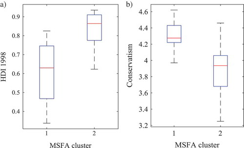
The comparison of MSFA models with different numbers of clusters and two factors per cluster indicated that, in general, the same two extreme factor structures were always found, with the additional clusters only leaving more room for setting apart data blocks with an intermediate factor structure. Thus, we select the MSFA model with two clusters and two factors per cluster. The clustering of the selected model is given in Table 2. Most countries are assigned to the clusters with a posterior probability of 1, whereas a negligible amount of classification uncertainty is found for Slovakia and South Africa. To validate and interpret the obtained clusters, we looked into some demographic measures that were available on the countries. An interesting difference between the clusters pertained to the Human Development Index (HDI) 1998, which was available from the Human Development Report 2000 (United Nations Development Program, 2000) for 47 out of the 48 countries in the ICS study (i.e., only lacking for Kuwait). The HDI takes on values between 0 and 1 and measures the average achievements in a country in terms of life expectancy, knowledge, and a decent standard of living. Figure 2a depicts boxplots of the HDI per cluster and shows that Cluster 1 contains less developed countries. Another aspect distinguishing the clusters was the level of conservatism (Schwartz, 1994), which was available for only half of the countries. Conservatism corresponds to a country’s emphasis on maintaining the status quo, propriety, and restraining actions or desires that might disrupt group solidarity or traditional order. Specifically, as Figure 2b shows, the countries in Cluster 1 are more conservative than the ones in Cluster 2.

TABLE 2 Clustering of the Countries of the Mixture Simultaneous Factor Analysis Model With Two Clusters and Two Factors Per Cluster for the Emotion Norm Data From the 2001 ICS Study

Cluster 1	Bangladesh, Brazil, Bulgaria, Cameroon, Georgia, Ghana, India, Iran, Nepal, Nigeria, Slovakia (= .9980), South Africa (= .9965), Thailand, Turkey, Uganda, Zimbabwe
Cluster 2	Australia, Austria, Belgium, Canada, Chile, China, Colombia, Croatia, Cyprus, Egypt, Germany, Greece, Hong Kong, Hungary, Indonesia, Italy, Japan, Kuwait, Malaysia, Mexico, Netherlands, Philippines, Poland, Portugal, Russia, Singapore, Slovenia, South Korea, Spain, Switzerland, United States, Venezuela

Note. Except for Slovakia and South Africa, all countries are assigned to the clusters with a posterior probability of 1. The probabilities for Slovakia and South Africa are given in brackets.

FIGURE 2 Boxplots for (a) the Human Development Index (HDI) 1998 (United Nations Development Program, 2000) and (b) the level of conservatism (Schwartz, 1994) of the countries per cluster of the Mixture Simultaneous Factor Analysis model with two clusters and two factors per cluster for the International College Survey data set on emotion norms.

To shed light on how the covariance structure of emotion norms differs between the conservative and less developed countries on the one hand and the progressive and developed countries on the other hand, we first look at the Varimax rotated cluster-specific factor loading matrices in Table 3. As expected, the two factors correspond to positive or approved and negative or disapproved emotions, respectively, and they do so in both clusters, indicating that the within-country covariance structures have much in common. In addition to slight differences in the size of primary and secondary loadings, the most important and interesting cross-cultural difference is found with respect to pride. Specifically, in Cluster 1, the primary loading of pride is on the negative factor, whereas, in Cluster 2, its primary loading is on the positive factor. Thus, by applying MSFA, we conveniently learned that in the conservative and less developed countries of Cluster 1, pride is a disapproved emotion, whereas in the progressive, developed countries of Cluster 2, pride is more positively valued by society. Possibly in Cluster 1 pride is considered to be an expression of arrogance and superiority, whereas in Cluster 2 it is regarded as a sign of self-confidence, which is a valued trait in progressive and developed countries. To complete the picture of the covariance differences, the cluster-specific unique variances are given in Table 4. From Table 4, it is apparent that all items have a higher unique variance in Cluster 2, implying that they have more idiosyncratic variability in the progressive, developed countries.

TABLE 3 Varimax (Top) and Echelon (Bottom) Rotated Loadings of the Mixture Simultaneous Factor Analysis Model With Two Clusters and Two Factors Per Cluster for the Emotion Norm Data From the 2001 ICS Study

	Cluster 1		Cluster 2
Varimax Rotation	Positive	Negative	Positive	Negative
Contentment	1.44	−0.25	1.21	−0.11
Happy	1.60	−0.26	1.42	−0.15
Love	1.39	−0.26	1.22	−0.06
Sad	−0.32	1.32	0.05	1.26
Jealousy (in romantic situations)	0.00	1.29	−0.02	1.27
Cheerful	1.18	−0.30	1.04	−0.05
Worry	−0.07	1.74	0.04	1.43
Stress	−0.25	2.01	−0.19	1.69
Anger	−0.37	1.97	−0.18	1.54
Pride	0.27	1.10	0.60	0.35
Guilt	0.05	1.24	0.11	1.10
Shame	0.18	1.03	0.08	1.07
Gratitude	0.95	−0.29	0.86	−0.12
	Cluster 1		Cluster 2
Echelon Rotation	Positive	Negative	Positive	Negative
Contentment	1.44**	−0.25	1.21**	−0.13
Happy	1.60**	−0.26	1.42**	−0.17
Love	1.39*	−0.26	1.22*	−0.08
Sad	−0.32**	1.32	0.07**	1.26
Jealousy (in romantic situations)	0	1.29	0	1.27
Cheerful	1.18	−0.30*	1.04	−0.06*
Worry	−0.07	1.74**	0.07	1.43**
Stress	−0.25	2.01**	−0.16	1.69**
Anger	−0.37	1.97**	−0.16	1.54**
Pride	0.27**	1.10**	0.61**	0.34**
Guilt	0.05	1.24	0.13	1.10
Shame	0.18	1.03	0.10	1.07
Gratitude	0.95	−0.29	0.86	−0.14

Note. For each emotion, the primary loading is shown in bold. Below, the restricted loadings are in italic and underlined and loadings that are significantly different across clusters (according to Wald tests and after Bonferroni correction) are indicated by **p < .01 and *p < .05.

TABLE 4 Unique Variances of the Mixture Simultaneous Factor Analysis Model With Two Clusters and Two Factors Per Cluster for the Emotion Norm Data From the 2001 ICS Study

	Cluster 1	Cluster 2
Contentment	1.47	3.48
Happy	0.63	1.39
Love	1.21	2.37
Sad	2.76	4.19
Jealousy (in romantic situations)	2.85	4.94
Cheerful	1.53	2.38
Worry	2.01	2.86
Stress	2.15	2.63
Anger	1.87	2.23
Pride	3.41	5.33
Guilt	2.80	4.42
Shame	3.01	4.85
Gratitude	2.88	3.95

In addition to the visual comparison of the cluster-specific loadings (and unique variances), hypothesis testing is useful to discern which differences are significant or not. By default, LG provides the user with results of Wald tests for factor loading differences across clusters (Vermunt & Magidson, 2013). We need to eliminate the rotational freedom of the cluster-specific factors for these results to make sense, however. This can be done by a sensible set of loading restrictions such as echelon rotation (Dolan et al., 2009; McDonald, 1999) and choosing these restrictions is easier in the case of less clusters and less factors per cluster. In Table 3, we see that jealousy has a loading of (almost) zero in both clusters. Restricting this loading to be exactly zero in both clusters imposes echelon rotation and solves the rotational freedom. The resulting cluster-specific loadings are given in the lower portion of Table 3 and they hardly differ (i.e., the difference is never larger than .03) from the Varimax rotated ones. As indicated in Table 3, 8 factor loadings are significantly different between the clusters at the 1% level, whereas 10 are significantly different at the 5% level (Bonferroni correction for multiple testing was applied).⁵

DISCUSSION

In this article, we presented MSFA, a novel exploratory method for clustering groups (i.e., higher level units or data blocks, in general) with respect to the underlying factor loading structure as well as their unique variances. When researchers have statistical, empirical, or theoretical reasons to expect possible differences, MSFA provides a solution to evaluate which differences exist and for which blocks. The solution is parsimonious because of the clustering of the data blocks, implying that only a few cluster-specific factor loading matrices need to be compared to pinpoint the differences in factor structure. Moreover, the clustering is often an interesting result in itself.

In this article, the MSFA model was specified as the exact stochastic counterpart of the clusterwise SCA variant described by De Roover, Ceulemans, Timmerman, Vansteelandt, (2012), that is, with block-specific factor (co)variance matrices equal to identity, such that all differences in observed-variable covariances are captured between the clusters by their cluster-specific factor loading matrices. Of course, in some cases, more flexible specifications are preferable; for instance, when one wants data blocks with the same factors but different factor (co)variances to be assigned to the same cluster. Another alternative model specification might include block-specific intercepts, instead of using data block centering, thus preserving information on block-specific mean levels and capturing them in the model.

In contrast to clusterwise SCA, MSFA provides information on classification uncertainty, when present. Also, common variance is distinguished from unique variance (including measurement error). Thus, in specific cases wherein the unique variances differ strongly between variables, between clusters, or both, MSFA will capture the underlying latent structures and the corresponding clustering more accurately. When this is not the case, clusterwise SCA might give similar results.

Of course, when pursuing inferential conclusions, the stochastic framework is to be preferred. For instance, it might be interesting to look at the standard errors of the parameter estimates. More important, with respect to the factor loading differences, one could argue that visual comparison of the cluster-specific loadings is too subjective. Conveniently, hypothesis testing for factor loading differences is available within the stochastic framework of MSFA and in LG. As stated earlier, these inferential tools are not yet readily applicable for MSFA, which is due to the rotational freedom of the cluster-specific factors. For now, for the standard errors and Wald test results to make sense, rotational freedom can be eliminated by imposing loading restrictions, as was illustrated earlier. To avoid this choice of restrictions and its possible influence on the clustering, standard error estimation should be combined with the specification of rotational criteria for the cluster-specific factor structures. It is important to note that the factor rotation of choice affects which differences are found between the clusters, be it visually or by means of hypothesis testing. Therefore, future research will include evaluating the influence and suitability of different rotational criteria. Rotational criteria pursuing both between-cluster agreement and simple structure of the loadings seem appropriate (Kiers, 1997; Lorenzo‐Seva, Kiers, & Berge, 2002) and the criteria can be converted into loading constraints to be imposed directly during maximum likelihood estimation (Archer & Jennrich, 1973; Jennrich, 1973).

The rotational freedom per cluster is a consequence of our choice for an exploratory approach (i.e., using EFA instead of CFA per cluster). Developing an MSFA variant with CFA within the clusters might be interesting for very specific cases like imposing the Big Five structure of personality for one cluster and the Big Three for the other cluster (De Raad et al., 2010) to see which countries end up in which cluster. Note that a priori assumptions on the underlying factor structure(s) can also be useful for the current, exploratory MSFA; that is, as a target structure when rotating the cluster-specific factor structures and when selecting the number of factors.

Finally, the obtained factor loading differences and clusters depend on the number of clusters as well as the number of factors within the clusters. Therefore, solving the so-called model selection problem is imperative. To this end, the performance of the BIC for MSFA model selection will be thoroughly evaluated and adaptations will be explored if needed. The fact that the BIC performance needs to be scrutinized is illustrated by the fact that, for the application, the BIC selected seven clusters, which appears to be an overselection when comparing cluster-specific factors and considering the (lack of) interpretability and stability of the clustering. Adaptations that will be considered include the hierarchical BIC (Zhao, Jin, & Shi, 2015; Zhao, Yu, & Shi, 2013) and stepwise procedures like the one described by Lukočienė, Varriale, and Vermunt (2010). Their performances will be investigated and compared, also for the more intricate case wherein the number of factors might vary across clusters.

FUNDING

Kim De Roover is a post-doctoral fellow of the Fund for Scientific Research Flanders (Belgium). The research leading to the results reported in this article was sponsored in part by Belgian Federal Science Policy within the framework of the Interuniversity Attraction Poles program (IAP/P7/06), by the Research Council of KU Leuven (GOA/15/003), and by the Netherlands Organization for Scientific Research (NWO; Veni grant 451-16-004).

Additional information

Funding

The research leading to the results reported in this article was sponsored in part by Belgian Federal Science Policy within the framework of the Interuniversity Attraction Poles program (IAP/P7/06), by the Research Council of KU Leuven (GOA/15/003), and by the Netherlands Organization for Scientific Research (NWO; Veni grant 451-16-004).

Notes

¹ Note that multilevel EFA (Muthén, 1991) models the pooled within-block covariance structure and the covariance structure of the block-specific means by lower and higher level factors, respectively. A connection between equality of the lower versus higher order factor structure and invariance of within-block factors across data blocks has been shown (Jak, Oort, & Dolan, 2013), however.

² An alternative would be to include block-specific (rather than cluster-specific) means in the model. This does not affect the obtained solution.

³ Allowing for a different number of factors across the clusters complicates the comparison of cluster-specific models and implies a severe model selection problem (e.g., De Roover, Ceulemans, Timmerman, Nezlek, & Onghena, 2013) that needs to be scrutinized in future research.

⁴ The congruence coefficient (Tucker, 1951) between two column vectors x and y is defined as their normalized inner product: .

⁵ Note that Wald test results are also available for differences in unique variances. For the emotion norm data set, all between-cluster differences in unique variances were significant at the 1% level.

APPENDIX A

MAXIMUM LIKELIHOOD ESTIMATION OF MSFA BY LG 5.1

In this appendix, we consecutively elaborate on the MSFA algorithm and the multistart procedure that we recommend using. An example of the syntax for estimating an MSFA model in LG 5.1. is given and clarified in Appendix B.

Algorithm

Two of the most common algorithms for ML estimation are EM (Dempster, Laird, & Rubin, 1977) and NR (Jennrich & Sampson, 1976). In LG, a combination of both types of iterations is applied to benefit from the stability of EM when it is far from the maximum of log L, and the convergence speed of NR when it is close to the maximum (Vermunt & Magidson, 2013).

Expectation-maximization lterations

As in all mixture models, log L (Equation 3)—also referred to as the observed-data log-likelihood—is complicated by the latent clustering of the data blocks, making it hard to maximize log L directly. Therefore, the EM algorithm makes use of the so-called complete-data (log)likelihood; that is, the likelihood when the cluster memberships of all data blocks are assumed to be known or, in other words, the joint distribution of the observed and latent data:

(A.1)

where Z is the I × K latent membership matrix, containing binary elements z_ik to indicate the cluster memberships. The probability density of the observed data conditional on the latent data is defined as follows:

(A.2)

and the probability density of the latent cluster memberships, or the so-called prior distribution of the latent clustering, is given by a multinomial distribution such that:

(A.3)

with the mixing proportions as the prior cluster probabilities. When data block i belongs to cluster k (z_ik = 1), the corresponding factors in Equations A.2 and A.3 remain unchanged and, when the data block doesn’t belong to cluster k (z_ik = 0), they become equal to 1. Inserting Equations A.2 and A.3 into Equation A.1 leads to a complete-data likelihood function containing no summation. Therefore, the complete-data log-likelihood or log L_c can be elaborated as follows:

(A.4)

From the summations in Equation A.4, we conclude that one difficult maximization (i.e., of Equation 3) is replaced by a sequence of easier maximization problems (see M-step of the EM procedure). Because the values of z_ik are unknown, their expected values—that is, the posterior classification probabilities (Equation 2)—are inserted in Equation A.4, thus obtaining the expected value of log L_c or E(log L_c). Note that log L can be obtained by summing E(log L_c) over the K possible latent cluster assignments for each data block.

Starting from a set of initial values for the parameters, the EM procedure performs the following two steps for each iteration :

E-step: The E(log L_c) value given the current parameter estimates (i.e., when = 1 or the estimates from the previous iteration when > 1) is determined as follows:

The posterior classification probabilities are calculated (Equation 2).

The values are inserted into Equation A.4 to obtain E(log L_c) for .

M-step: The parameters are estimated such that E(log L_c) is maximized. Note that this also results in an increase with respect to log L (Dempster et al., 1977).

An update of each —satisfying —is given by (McLachlan & Peel, 2000):

(A.5)

For each cluster k, the factor model for is obtained by weighting each observation by the corresponding value and performing factor analysis on the weighted data. To this end, a separate EM algorithm (Rubin & Thayer, 1982) can be used or one of the alternatives described by Lee and Jennrich (1979). Currently, LG uses Fisher scoring to estimate the cluster-specific factor models. Fisher scoring (Lee & Jennrich, 1979) is an approximation of the NR procedure described next.

Newton–Raphson iterations

In contrast to EM, NR optimization operates directly on log L (Equation 3). Specifically, NR iteratively maximizes an approximation of log L, based on its first- and second-order partial derivatives, in the point corresponding to estimates . Using these derivatives, NR updates all model parameters at once. The first-order derivatives—with respect to parameters , r = 1, …, R—are gathered in the so-called gradient vector g:

(A.6)

where R is equal to for MSFA with orthogonal factors. The gradient vector indicates the direction of the greatest rate of increase in log L, where element g_r is positive when higher values of log L can be found at higher values of θ_r and negative otherwise. The derivations of the elements of the gradient for an MSFA model are given in the next section.

The matrix of second-order derivatives—also called the Hessian or H—contains the following elements:

(A.7)

where H_rs refers to the element in row r and column s of H. Geometrically, the second-order derivatives refer to the curvature of the R-dimensional log-likelihood surface. Taking the curvature into account makes the update more efficient than an update based on the gradient alone (Battiti, 1992). H and g are combined in the NR update as follows:

(A.8)

where the stepsize ε, 0 < ε < 1, is used to prevent a decrease in log L whenever a standard NR update causes a so-called overshoot (for details, see Vermunt & Magidson, 2013). The calculations of the second-order derivatives make the NR update computationally very expensive. Therefore, LG applies an approximation of the Hessian, which is given in the next section.

First- and second-order derivatives of observed-data log-likelihood

The first-order derivative of log L can be decomposed as:

(A.9)

where is the log-likelihood contribution of cluster k. When defining the expected observed number of blocks and number of observations in cluster k as and respectively, log L_k can be expressed in terms of the cluster-specific expected observed covariance matrix as follows:

(A.10)

The first derivative of thus becomes the following (Magnus & Neudecker, 2007):

(A.11)

such that The second-order derivative of is then equal to (Magnus & Neudecker, 2007):

(A.12)

Because the expected value of equals zero, the expected value of the second derivative of becomes . Therefore, within LG, the second-order derivative of log L is approximated as:

(A.13)

Convergence

In practice, the estimation process starts with a number of EM iterations. When close to the final solution, the program switches to NR iterations to speed up convergence. Convergence can be evaluated with respect to log L or with respect to the parameter estimates. LG applies the latter approach (Vermunt & Magidson, 2013). More specifically, convergence is evaluated by computing the following quantity:

(A.14)

which is the sum of the absolute value of the relative changes in the parameters. The convergence criterion that is used for MSFA in this article is < 1 × 10⁻⁸. The iteration also stops when the change in log L is negligible; that is, smaller than 1 × 10⁻¹².

It is important to note that, when convergence is reached, this is not necessarily a global maximum. To increase the probability of finding the global maximum, a multistart procedure is used, which is described in the next section.

Multistart Procedure

LG applies a tiered testing strategy with respect to sets of starting values (Vermunt & Magidson, 2013). Specifically, it starts from a user-specified number of sets (say 25), each of which is updated for a maximum number of iterations (e.g., 100) or until is smaller than a specified criterion (e.g., 1 × 10^–5). Subsequently, it continues with the 10% (rounded upward) most promising sets (i.e., with the highest log L), performing another two times the specified number of iterations (e.g., 2 × 100). Finally, it continues with the best solution until convergence. Note that such a procedure increases considerably the probability of finding the global ML solution, but does not guarantee it. Thus, one should remain cautious of local maxima.

With respect to generating sets of starting values, a special option was added to the LG 5.1 syntax module to create suitable initial values for the cluster-specific loadings and unique variances of MSFA. Specifically, the initial values are based on the loadings and residual variances of a principal component (PCA) model (Jolliffe, 1986; Pearson, 1901), in principal axes position, for the entire data set. This seems reasonable as typically loadings from PCA strongly resemble the ones of EFA (Widaman, 1993). To create K sufficiently different sets of initial factor loadings, randomness is added to the PCA loadings for each cluster k:

(A.15)

where rand(1) indicates a J × Q matrix of random numbers sampled from a uniform distribution between 0 and 1, and ‘*’ denotes the elementwise product. Note that the default random seed is based on time, such that the added random numbers will be unique for each set of starting values (Vermunt & Magidson, 2013). To avoid the occurrence of Heywood cases (Rindskopf, 1984; Van Driel, 1978) very early in the model estimation, the initial unique variances are generated as follows:

(A.16)

where diag(D_k) refers to the diagonal elements of D_k and var(E_PCA) denotes the variances of the PCA residuals. Preliminary simulation studies indicated a much lower sensitivity to local maxima and a faster computation time when using these starting values instead of mere random values.

APPENDIX B

LATENT GOLD 5.1 SYNTAX FOR MSFA ANALYSIS

The LG syntax is built up from three sections: ‘options,’ ‘variables,’ and ‘equations.’ First, the ‘options’ section pertains to specifications regarding the estimation process and to output options. The parameters in the ‘algorithm’ subsection indicate when the algorithm should proceed with NR instead of EM iterations and when convergence is reached (see Vermunt & Magidson, 2013). The ‘startvalues’ subsection includes the parameters pertaining to the multistart procedure. Specifically, for each set of starting values (the number of sets is specified by ‘sets’), the model is reestimated for as many iterations as specified by ‘iterations’ or until drops below the ‘tolerance’ value. Then, the multistart procedure proceeds as described in Appendix A. ‘PCA’ prompts LG to use the PCA-based starting values, whereas otherwise ‘seed = 0’ would give the default random starts (for other possible ‘seed’ values, see Vermunt & Magidson, 2013). In the ‘output’ and ‘outfile’ subsections, the desired output can be specified by the user (for more details, see Vermunt & Magidson, 2013). The parameters of the remaining subsections are not used in this article.

Second, the ‘variables’ section specifies the different types of variables included in the model. Because MSFA operates on multilevel data, after ‘groupid,’ the variable in the data file that specifies the group structure (i.e., the data block number for each observation) should be specified (e.g., ‘V1’), using its label in the data file. In the ‘dependent’ subsection, the dependent variables of the model (i.e., the observed variables) should be specified, by means of their label in the data file and their measurement scale. Next, the ‘independent’ variables can be specified. In the MSFA case, it is useful to include the grouping variable as an independent variable to get the cluster memberships per data block rather than per row (i.e., in the ‘probmeans-posterior’ output tab; Vermunt & Magidson, 2013). Finally, the ‘latent’ variables of the MSFA model are the factors (i.e., ‘F1’ to ‘F4’ in the example syntax) and the mixture model clustering (i.e., ‘Cluster’). In particular, the former are specified as continuous latent variables, whereas the latter is specified as a nominal latent variable at the group level with a specified number of categories (i.e., the desired number of clusters). By ‘coding = first’ Cluster 1 is (optionally) coded as the reference cluster in the logistic regression model for the clustering (explained later). For other coding options, see Vermunt and Magidson (2013).

In the ‘equations’ section, the model equations are listed. First, the factor variances are specified and fixed at one. No factor covariances are specified, implying that orthogonal factors are estimated. Note that both restrictions apply to each data block, because we do not specify an effect of the grouping variable on the factor (co)variances. Next, a logistic regression model for the categorical latent variable ‘Cluster’ is specified (Vermunt & Magidson, 2013), which contains only an intercept term in case of MSFA. Specifically, this intercept vector relates to the prior probabilities or mixing proportions of the clusters in that it includes the odds ratios for the K − 1 nonreference clusters with respect to the reference cluster; that is, Cluster 1:

(B.1)

Then, regression models are defined for the observed variables; that is, which variables are regressed on which factors. Note that, for MSFA, all variables are regressed on all factors (i.e., it applies EFA) and that no intercept term is included. By default, overall factor means are equal to zero and no effect is specified to make them differ between data blocks or clusters. To obtain factor loadings that differ between the clusters, ‘|Cluster’ is added to each regression effect. Finally, item variances are added, which pertain to the unique variances in this case and which are also allowed to differ across clusters. Optionally, at the end of the syntax, additional restrictions might be specified or starting values for all parameters might be given, either by directly typing them in the syntax or by referring to a text file (see Vermunt & Magidson, 2013).

APPENDIX CLATENT GOLD 5.1 SYNTAX FOR MSFA SIMULATION

For generating the simulated data sets by means of LG, syntaxes were used like the one shown here. The cluster memberships, the data block sizes (i.e., the number of rows per block), as well as the number of variables (including a variable to identify the data blocks) were communicated to the simulation syntax by means of a text file (Figure C.1), which is referred to as the ‘example’ file in the LG manual (Vermunt & Magidson, 2013). The observed variables are still to be simulated and can thus take on arbitrary but admissible values in the example file; in this simulation study, random numbers from a standard normal distribution were used. The simulation syntax lists a lot of technical parameters in the ‘Options’ section. Most of them are discussed in Appendix B. The ‘outfile simulateddata.txt simulation’ option will generate one simulated data set from the population model that is specified further on in the syntax, and will save it as a text file. The montecarlo parameters pertain to other types of simulation studies and resampling studies (see Vermunt & Magidson, 2013). The MSFA population model encompasses a model syntax (see Appendix B) and ‘starting values’ for all free model parameters (i.e., the population-level parameter values that were written into a text file, with, per cluster, first the unique variances and then the loadings of the first factor, followed by the loadings of the second factor, and so on). The model syntax determines the data block structure of the data to be simulated by the ‘groupid’ and ‘caseweight’ variable. An important difference with an analysis is that, when simulating, the clustering is known (through the example file) and it is thus defined as an independent variable in the simulation syntax model.

FIGURE C.1  ‘Example.txt’ file communicating the clustering (‘Cluster’), the number of variables (‘V2’ to ‘V13’) and the data block structure (‘V1’ and ‘rows’) to the simulation syntax for LG 5.1. Note that, in general, the number of rows can differ across data blocks.

REFERENCES

- Archer, C. O., & Jennrich, R. I. (1973). Standard errors for orthogonally rotated factor loadings. Psychometrika, 38, 581–592. doi:10.1007/BF02291496
- Asparouhov, T., & Muthén, B. (2014). Multiple-group factor analysis alignment. Structural Equation Modeling, 21, 495–508. doi:10.1080/10705511.2014.919210
- Battiti, R. (1992). First-and second-order methods for learning: Between steepest descent and Newton’s method. Neural Computation, 4, 141–166. doi:10.1162/neco.1992.4.2.141
- Blafield, E. (1980). Clustering of observations from finite mixtures with structural information. Jyvaskyla, Finland: Jyvaskyla University.
- Borsboom, D., Mellenbergh, G. J., & van Heerden, J. (2003). The theoretical status of latent variables. Psychological Review, 110, 203–219. doi:10.1037/0033-295X.110.2.203
- Brose, A., De Roover, K., Ceulemans, E., & Kuppens, P. (2015). Older adults’ affective experiences across 100 days are less variable and less complex than younger adults’. Psychology and Aging, 30, 194–208. doi:10.1037/a0038690
- Bulteel, K., Wilderjans, T. F., Tuerlinckx, F., & Ceulemans, E. (2013). CHull as an alternative to AIC and BIC in the context of mixtures of factor analyzers. Behavior Research Methods, 45, 782–791. doi:10.3758/s13428-012-0293-y
- De Raad, B., Barelds, D. P. H., Levert, E., Ostendorf, F., Mlačić, B., Di Blas, L., … Katigbak, M. S. (2010). Only three factors of personality description are fully replicable across languages: A comparison of 14 trait taxonomies. Journal of Personality and Social Psychology, 98, 160–173. doi:10.1037/a0017184
- De Roover, K., Ceulemans, E., & Timmerman, M. E. (2012). How to perform multiblock component analysis in practice. Behavior Research Methods, 44, 41−56. doi:10.3758/s13428-011-0129-1
- De Roover, K., Ceulemans, E., Timmerman, M. E., Nezlek, J. B., & Onghena, P. (2013). Modeling differences in the dimensionality of multiblock data by means of clusterwise simultaneous component analysis. Psychometrika, 78, 648–668. doi:10.1007/s11336-013-9318-4
- De Roover, K., Ceulemans, E., Timmerman, M. E., & Onghena, P. (2013). A clusterwise simultaneous component method for capturing within-cluster differences in component variances and correlations. British Journal of Mathematical and Statistical Psychology, 86, 81−102.
- De Roover, K., Ceulemans, E., Timmerman, M. E., Vansteelandt, K., Stouten, J., & Onghena, P. (2012). Clusterwise simultaneous component analysis for analyzing structural differences in multivariate multiblock data. Psychological Methods, 17, 100−119. doi:10.1037/a0025385
- de Winter, J. C. F., Dodou, D., & Wieringa, P. A. (2009). Exploratory factor analysis with small sample sizes. Multivariate Behavioral Research, 44, 147–181. doi:10.1080/00273170902794206
- Dempster, A. P., Laird, N. M., & Rubin, D. B. (1977). Maximum likelihood from incomplete data via the EM algorithm. Journal of the Royal Statistical Society: Series B (Methodological), 39, 1–38.
- Diener, E., Kim-Prieto, C., & Scollon, C., & Colleagues. (2001). [International College Survey 2001]. Unpublished raw data.
- Dolan, C. V., Oort, F. J., Stoel, R. D., & Wicherts, J. M. (2009). Testing measurement invariance in the target rotated multigroup exploratory factor model. Structural Equation Modeling, 16, 295–314. doi:10.1080/10705510902751416
- Dziak, J. J., Coffman, D. L., Lanza, S. T., & Li, R. (2012). Sensitivity and specificity of information criteria. PeerJ PrePrints, 3, e1350.
- Eid, M., & Diener, E. (2001). Norms for experiencing emotions in different cultures: Inter- and intranational differences. Journal of Personality and Social Psychology, 81, 869–885. doi:10.1037/0022-3514.81.5.869
- Ekman, P. (1999). Basic emotions. In T. Dalgleish & M. J. Power (Eds.), Handbook of cognition and emotion (pp. 45–60). Chichester, UK: Wiley.
- Fonseca, J. R., & Cardoso, M. G. (2007). Mixture-model cluster analysis using information theoretical criteria. Intelligent Data Analysis, 11, 155–173.
- Fontaine, J. R. J., Poortinga, Y. H., Setiadi, B., & Markam, S. S. (2002). Cognitive structure of emotion terms in Indonesia and the Netherlands. Cognition & Emotion, 16, 61–86.
- Fontaine, J. R. J., Scherer, K. R., Roesch, E. B., & Ellsworth, P. C. (2007). The world of emotions is not two-dimensional. Psychological Science, 18, 1050–1057. doi:10.1111/j.1467-9280.2007.02024.x
- Gorsuch, R. L. (1990). Common factor analysis versus component analysis: Some well and little known facts. Multivariate Behavioral Research, 25, 33–39. doi:10.1207/s15327906mbr2501_3
- Hessen, D. J., Dolan, C. V., & Wicherts, J. M. (2006). Multi-group exploratory factor analysis and the power to detect uniform bias. Applied Psychological Research, 30, 233–246.
- Hu, L., & Bentler, P. M. (1999). Cutoff criteria for fit indexes in covariance structure analysis: Conventional criteria versus new alternatives. Structural Equation Modeling, 6, 1–55. doi:10.1080/10705519909540118
- Hubert, L., & Arabie, P. (1985). Comparing partitions. Journal of Classification, 2, 193–218. doi:10.1007/BF01908075
- Jak, S., Oort, F. J., & Dolan, C. V. (2013). A test for cluster bias: Detecting violations of measurement invariance across clusters in multilevel data. Structural Equation Modeling, 20, 265–282. doi:10.1080/10705511.2013.769392
- Jennrich, R. I. (1973). Standard errors for obliquely rotated factor loadings. Psychometrika, 38, 593–604. doi:10.1007/BF02291497
- Jennrich, R. I., & Sampson, P. F. (1976). Newton–Raphson and related algorithms for maximum likelihood variance component estimation. Technometrics, 18, 11–17. doi:10.2307/1267911
- Jolliffe, I. T. (1986). Principal component analysis. New York, NY: Springer.
- Jöreskog, K. G. (1971). Simultaneous factor analysis in several populations. Psychometrika, 36, 409–426. doi:10.1007/BF02291366
- Kaiser, H. F. (1958). The Varimax criterion for analytic rotation in factor analysis. Psychometrika, 23, 187–200. doi:10.1007/BF02289233
- Kiers, H. A. (1997). Techniques for rotating two or more loading matrices to optimal agreement and simple structure: A comparison and some technical details. Psychometrika, 62, 545–568. doi:10.1007/BF02294642
- Kim, E. S., Joo, S. H., Lee, P., Wang, Y., & Stark, S. (2016). Measurement invariance testing across between-level latent classes using multilevel factor mixture modeling. Structural Equation Modeling, 23, 870–887. doi:10.1080/10705511.2016.1196108
- Krysinska, K., De Roover, K., Bouwens, J., Ceulemans, E., Corveleyn, J., Dezutter, J., … Pollefeyt, D. (2014). Measuring religious attitudes in secularized Western European context: A psychometric analysis of the Post-Critical Belief Scale. The International Journal for the Psychology of Religion, 24, 263–281. doi:10.1080/10508619.2013.879429
- Kuppens, P., Ceulemans, E., Timmerman, M. E., Diener, E., & Kim-Prieto, C. (2006). Universal intracultural and intercultural dimensions of the recalled frequency of emotional experience. Journal of Cross-Cultural Psychology, 37, 491–515. doi:10.1177/0022022106290474
- Lawley, D. N., & Maxwell, A. E. (1962). Factor analysis as a statistical method. The Statistician, 12, 209–229. doi:10.2307/2986915
- Lee, S. Y., & Jennrich, R. I. (1979). A study of algorithms for covariance structure analysis with specific comparisons using factor analysis. Psychometrika, 44, 99–113. doi:10.1007/BF02293789
- Lorenzo‐Seva, U., Kiers, H. A., & Berge, J. M. (2002). Techniques for oblique factor rotation of two or more loading matrices to a mixture of simple structure and optimal agreement. British Journal of Mathematical and Statistical Psychology, 55, 337–360. doi:10.1348/000711002760554624
- Lubke, G. H., & Muthén, B. (2005). Investigating population heterogeneity with factor mixture models. Psychological Methods, 10, 21. doi:10.1037/1082-989X.10.1.21
- Lukočienė, O., Varriale, R., & Vermunt, J. K. (2010). The simultaneous decision(s) about the number of lower‐ and higher‐level classes in multilevel latent class analysis. Sociological Methodology, 40, 247–283. doi:10.1111/j.1467-9531.2010.01231.x
- MacKinnon, N. J., & Keating, L. J. (1989). The structure of emotions: Canada–United States comparisons. Social Psychology Quarterly, 52, 70–83. doi:10.2307/2786905
- Magnus, J. R., & Neudecker, H. (2007). Matrix differential calculus with applications in statistics and econometrics (3rd ed.). Chichester, UK: Wiley.
- McDonald, R. P. (1999). Test theory: A unified treatment. Hillsdale, NJ: Lawrence Erlbaum Associates, Inc.
- McDonald, R. P., & Krane, W. R. (1979). A Monte Carlo study of local identifiability and degrees of freedom in the asymptotic likelihood ratio test. British Journal of Mathematical and Statistical Psychology, 32, 121–132. doi:10.1111/bmsp.1979.32.issue-1
- McLachlan, G. J., & Peel, D. (2000). Finite mixture models. New York, NY: Wiley.
- Muthén, B., & Asparouhov, T. (2013). BSEM measurement invariance analysis. Mplus Web Notes, 17, 1–48.
- Muthén, B. O. (1989). Latent variable modeling in heterogeneous populations. Psychometrika, 54, 557–585. doi:10.1007/BF02296397
- Muthén, B. O. (1991). Multilevel factor analysis of class and student achievement components. Journal of Educational Measurement, 28, 338–354. doi:10.1111/j.1745-3984.1991.tb00363.x
- Muthén, L. K., & Muthén, B. O. (2005). Mplus: Statistical analysis with latent variables. User’s guide. Los Angeles, CA: Muthén & Muthén.
- Ogasawara, H. (2000). Some relationships between factors and components. Psychometrika, 65, 167–185. doi:10.1007/BF02294372
- Pearson, K. (1901). On lines and planes of closest fit to systems of points in space. Philosophical Magazine, 2, 559–572. doi:10.1080/14786440109462720
- Rindskopf, D. (1984). Structural equation models empirical identification, Heywood cases, and related problems. Sociological Methods & Research, 13, 109–119. doi:10.1177/0049124184013001004
- Rodriguez, C., & Church, A. T. (2003). The structure and personality correlates of affect in Mexico: Evidence of cross-cultural comparability using the Spanish language. Journal of Cross Cultural Psychology, 34, 211–230. doi:10.1177/0022022102250247
- Rosseel, Y. (2012). Lavaan: An R package for structural equation modeling. Journal of Statistical Software, 48, 1–36. doi:10.18637/jss.v048.i02
- Rubin, D. B., & Thayer, D. T. (1982). EM algorithms for ML factor analysis. Psychometrika, 47, 69–76. doi:10.1007/BF02293851
- Russell, J. A., & Barrett, L. F. (1999). Core affect, prototypical emotional episodes, and other things called emotion: Dissecting the elephant. Journal of Personality and Social Psychology, 76, 805–819. doi:10.1037/0022-3514.76.5.805
- Schwartz, S. H. (1994). Beyond individualism/collectivism: New cultural dimensions of values. In U. Kim, H. C. Triandis, C. Kagitcibasi, S. C. Choi, & G. Yoon (Eds.), Individualism and collectivism: Theory, methods, and applications (pp. 85–119). Thousand Oaks, CA: Sage.
- Schwarz, G. (1978). Estimating the dimension of a model. The Annals of Statistics, 6, 461–464. doi:10.1214/aos/1176344136
- Sörbom, D. (1974). A general method for studying differences in factor means and factor structure between groups. British Journal of Mathematical and Statistical Psychology, 27, 229–239. doi:10.1111/bmsp.1974.27.issue-2
- Stearns, P. N. (1994). American cool: Constructing a twentieth-century emotional style. New York, NY: NYU Press.
- Steinley, D., & Brusco, M. J. (2011). Evaluating mixture modeling for clustering: Recommendations and cautions. Psychological Methods, 16, 63–79. doi:10.1037/a0022673
- Timmerman, M. E., & Kiers, H. A. L. (2003). Four simultaneous component models of multivariate time series from more than one subject to model intraindividual and interindividual differences. Psychometrika, 86, 105–122. doi:10.1007/BF02296656
- Tucker, L. R. (1951). A method for synthesis of factor analysis studies (Personnel Research Section Report No. 984). Washington, DC: Department of the Army.
- United Nations Development Program. (2000). Human development report 2000. New York, NY: Oxford University Press.
- Van Driel, O. P. (1978). On various causes of improper solutions in maximum likelihood factor analysis. Psychometrika, 43, 225–243. doi:10.1007/BF02293865
- Varriale, R., & Vermunt, J. K. (2012). Multilevel mixture factor models. Multivariate Behavioral Research, 47, 247–275. doi:10.1080/00273171.2012.658337
- Velicer, W. F., & Fava, J. L. (1998). Affects of variable and subject sampling on factor pattern recovery. Psychological Methods, 3, 231. doi:10.1037/1082-989X.3.2.231
- Velicer, W. F., & Jackson, D. N. (1990). Component analysis versus common factor analysis: Some issues in selecting an appropriate procedure. Multivariate Behavioral Research, 25, 1–28. doi:10.1207/s15327906mbr2501_1
- Velicer, W. F., Peacock, A. C., & Jackson, D. N. (1982). A comparison of component and factor patterns: A Monte Carlo approach. Multivariate Behavioral Research, 17, 371–388. doi:10.1207/s15327906mbr1703_5
- Vermunt, J. K., & Magidson, J. (2013). Technical guide for Latent GOLD 5.0: Basic, advanced, and syntax. Belmont, MA: Statistical Innovations.
- Widaman, K. F. (1993). Common factor analysis versus principal component analysis: Differential bias in representing model parameters? Multivariate Behavioral Research, 28, 263–311. doi:10.1207/s15327906mbr2803_1
- Yung, Y. F. (1997). Finite mixtures in confirmatory factor-analysis models. Psychometrika, 62, 297–330. doi:10.1007/BF02294554
- Zhao, J., Jin, L., & Shi, L. (2015). Mixture model selection via hierarchical BIC. Computational Statistics & Data Analysis, 88, 139–153. doi:10.1016/j.csda.2015.01.019
- Zhao, J., Yu, P. L., & Shi, L. (2013). Model selection for mixtures of factor analyzers via hierarchical BIC. Yunnan, China: School of Statistics and Mathematics, Yunnan University of Finance and Economics.