Relations between kinetic parameters of different column models for liquid chromatography applying core-shell particles

Abstract

This article presents analytical solutions of the general rate model (GRM), the lumped kinetic model (LKM), and the simpler equilibrium dispersive model (EDM) for core-shell particles and linear adsorption isotherms. The solutions in the Laplace domain are applied to derive analytical expressions for the temporal moments of these models. The results provide relations between the model specific kinetic parameters by matching one or more of the temporal moments. Several case studies are considered for illustration. The results show that simpler models are in many cases as good as the most detailed GRM if their kinetic parameters fulfill the matching relations. Thus, it is possible to reliably predict elution profiles using the simpler models. The derived analytical expressions can also be utilized to efficiently estimate model parameters from experimentally observed elution profiles to further optimize core-shell particles and to identify suitable column sizes and operating conditions.

Graphical Abstract

Keywords:

• Core-shell particles
• Liquid chromatography
• mathematical models
• moment analysis
• matching relations
• semi-analytical solutions

Introduction

Mathematical modeling is an essential part of the chromatographic theory for simulating its dynamical process. Several chromatographic models exist in the literature considering different levels of complexities to describe the process. The models, which are most frequently used in the simulation of liquid chromatography, are the general rate model (GRM), the lumped kinetic model (LKM), and the equilibrium dispersive model (EDM).^[1,2] Hereby, the GRM is the most detailed model, while the LKM and EDM have less degrees of freedom and are simpler. It accounts for various mass transfer kinetics that influence the band profiles, namely external mass transfer resistance and intraparticle diffusion. In addition axial dispersion is considered. Under linear conditions the model describes these effects with three kinetic parameters. The simpler LKM applies a linear driving force in the solid phase and considers just one additional parameter complementing the axial dispersion coefficient instead of considering the full intraparticle concentration profile. It lumps together the contributions of internal and external mass transport resistances within a single mass transfer coefficient and contains only two essential kinetic parameters, namely the axial dispersion and the mass transfer coefficient. The EDM is the most simple model that Lumps together all kinetic effects into a single apparent dispersion coefficient. It is well known that simpler models can be derived from the detailed GRM under certain simplifying assumptions.^[1–4]

The demand for increased efficiency during the last years triggered the development of cored beads, made up of a solid silica core and a porous thin shell. These particles have recently gathered considerable attention because of their unusual high column efficiencies, low column pressures and fast separation. They were invented and pioneered with the specific purpose of preparing columns that could provide highly efficient HPLC separation of high molecular weight compounds of biological origin.^[5] A comprehensive review describing” trials,tribulations and triumphs” was published by Guiochon and Gritti.^[6] Several authors other have theoretically investigated chromatographic columns packed with core-shell particles.^[7–19]

In our previous articles, we have derived analytical solutions and temporal moments of the EDM, LKM and GRM for columns packed with fully porous particles.^[20–22] Recently, we have also derived analytical solutions and moments of the linear GRM for core-shell particles.^[23] In all these derivations, the Laplace transformation was applied as a basic tool to derive analytical solutions. As analytical Laplace inversion was not possible in most of the cases. The numerical Laplace inversion was applied to back transform solutions in the actual time domain.^[24,25] The Laplace domain solutions were further utilized to derive analytical temporal moments. These moments can be used to measure retention times, band broadenings, front asymmetries and kurtosis of the elution profiles. Moment analysis and matching is well-known and instructive in the literature,^{[2,23,26–39]} and references therein. A high resolution finite volume scheme (HRFVS) was also applied to numerically approximate the linear and nonlinear GRM for fully-porous and core-shell particles.^[23,40]

This manuscript focuses on the derivation of relations among the essential kinetic parameters of the GRM and the two simpler LKM and EDM models for usage of columns packed with core-shell particles. These relations are derived by matching the corresponding temporal moments of the mentioned three models for linear isotherms.

The remaining parts of this manuscript are organized as follows. In Section 2 we start with the detailed GRM and then present the simpler LKM and EDM for core-shell particles. Section 3 refers the reader to Appendix A and Table 1 for the analytical solutions and temporal moments of the considered models, respectively. Section 4 presents relations between the kinetic parameters of these models after matching their corresponding moments. In Section 5, different numerical test problems are presented. Conclusions are drawn in Section 6.

Table 1. Analytical moments of GRM, LKM and EDM for core-shell particles (except $\mu {\prime }_4$ of GRM). Here, the zeroth moment ${\mu }_0=c_{ \text{inj}}{\tau }_{ \text{inj}}$, representing the amount injected, is the same for all models.

Moments	GRM	LKM (or EDM when $k_{\text{LKM}}\to \infty$ and $\mathit{Pe}=\frac{\mathit{Lu}}{D_{\text{app}}}$)
μ1	$$\frac{{\tau }_{\text{inj}}}{2}+\left(1+{\tilde{a}}^{*}{F}_e\right)$$	$$\frac{{\tau }_{\text{inj}}}{2}+\left(1+\tilde{a}{F}_e\right)$$
$\mu {\prime }_2$	$$\frac{{\tau }_{\text{inj}}^2}{12}+\frac{2}{\mathit{Pe}}{\left(1+{\tilde{a}}^{*}{F}_e\right)}^2+2F_e{({\tilde{a}}^{*})}^2\left[\frac{F_e}{\xi }+\frac{1}{15{\eta }_{\text{mod}}}\right]$$	$$\frac{{\tau }_{\text{inj}}^2}{12}+\frac{2}{\mathit{Pe}}{\left(1+\tilde{a}{F}_e\right)}^2+\frac{2\tilde{a}{F}_e^2{ϵ}_e}{{\kappa }_{\text{LKM}}}$$
$\mu {\prime }_3$	$$\frac{12}{P{e}^2}{\left(1+{\tilde{a}}^{*}{F}_e\right)}^3+\frac{6(1+{\tilde{a}}^{*}{F}_e)F_e}{\mathit{Pe}}\left[\frac{2F_e{({\tilde{a}}^{*})}^2}{\xi }+\frac{2{({\tilde{a}}^{*})}^2}{15{\eta }_{\text{mod}}}\right]$$	$$\frac{12}{P{e}^2}{\left(1+\tilde{a}{F}_e\right)}^3+\frac{12}{\mathit{Pe}}\frac{\left(1+\tilde{a}{F}_e\right){ϵ}_e\tilde{a}{F}_e^2}{{\kappa }_{\text{LKM}}}+\frac{6{ϵ}_e^2\tilde{a}{F}_e^3}{{\kappa }_{\text{LKM}}^2}$$
	$$+F_e{({\tilde{a}}^{*})}^3\left[\frac{4}{105{\eta }_{\text{mod}}^2}\frac{(1+{\rho }_2)}{{(1+{\rho }_1)}^2}+\frac{4F_e}{5\xi {\eta }_{\text{mod}}}+\frac{6F_e^2}{{\xi }^2}\right]$$
$\mu {\prime }_4$	$$\frac{12{\left(1+a^{*}{F}_e\right)}^4}{P{e}^4}\left[P{e}^2+10Pe\right]-\frac{4}{175}\frac{F_e^2{a}^{*4}\left(2+\mathit{Pe}\right)}{{\eta }^{2}Pe}$$	$$\frac{{\tau }_{\text{inj}}^4}{80}+{\tau }_{\text{inj}}^2\left[\frac{1}{\mathit{Pe}}{(1+\tilde{a}{F}_e)}^2+\frac{{ϵ}_e\tilde{a}{F}_e^2}{{\kappa }_{\text{LKM}}}\right]$$
	$$+\frac{24{(1+a^{*}{F}_e)}^2{F}_e{a}^{*2}}{P{e}^3}\left(\frac{F_e}{\xi }+\frac{1}{15\eta }\right)\left[P{e}^2+6Pe\right]$$	$$+\frac{12{\left(1+\tilde{a}{F}_e\right)}^4}{P{e}^4}\left[P{e}^2+10Pe\right]+\frac{24{ϵ}_e\tilde{a}{F}_e^2{\left(1+\tilde{a}{F}_e\right)}^2}{P{e}^3{\kappa }_{\text{LKM}}}\left[P{e}^2+6Pe\right]$$
	$$+\frac{2F_e{a}^{*3}}{\mathit{Pe}}\left(\frac{4}{105{\eta }^2}+\frac{4F_e}{5\xi \eta }+\frac{6F_e^2}{{\xi }^2}\right)\left[4+a^{*}{F}_e(6+\mathit{Pe})\right]$$	$$+\frac{12{ϵ}_e{}^2\tilde{a}{F}_e^3}{\mathit{Pe}{\kappa }_{\text{LKM}}^2}\left[4+\tilde{a}F(6+\mathit{Pe})\right]+\frac{24{ϵ}_e{}^3\tilde{a}{F}_e^4}{{\kappa }_{\text{LKM}}^3}$$
	$$+8F_e{a}^{*4}\left(\frac{1}{525}\frac{1}{{\eta }^3}+\frac{9}{175}\frac{F_e}{{\eta }^2\xi }+\frac{3}{5}\frac{F_e^2}{\eta {\xi }^2}+\frac{3F_e^3}{{\xi }^3}\right)$$
	$$+\frac{{\tau }_{\text{inj}}^4}{80}+{\tau }_{\text{inj}}^2\left[\frac{{(1+a^{*}{F}_e)}^2}{\mathit{Pe}}+F_e{a}^{*2}\left(\frac{F_e}{\xi }+\frac{1}{15\eta }\right)\right]$$
	(valid only for fully-porous particles)

$${\eta }_{\text{mod}}=\frac{\eta }{{\rho }_{\text{mod}}},\hspace{1em}{\rho }_{\text{mod}}=\frac{1+2{\rho }_{\text{core}}+3{\rho }_{\text{core}}^2-{\rho }_{\text{core}}^3-5{\rho }_{\text{core}}^4}{{(1+{\rho }_{\text{core}}+{\rho }_{\text{core}}^2)}^2},\hspace{1em}{\rho }_1=\frac{{\rho }_{\text{core}}(1+3{\rho }_{\text{core}}+3{\rho }_{\text{core}}^2-{\rho }_{\text{core}}^3)}{{(1+{\rho }_{\text{core}}+{\rho }_{\text{core}}^2)}^2},\hspace{1em}{\rho }_2=\frac{{\rho }_{\text{core}}(2+9{\rho }_{\text{core}}+\frac{35}{2}{\rho }_{\text{core}}^2+\frac{23}{2}{\rho }_{\text{core}}^3-3{\rho }_{\text{core}}^4-{\rho }_{\text{core}}^5)}{{(1+{\rho }_{\text{core}}+{\rho }_{\text{core}}^2)}^3},$$

$${\tilde{a}}^{*}=[{ϵ}_p+(1-{ϵ}_p\left)a\right](1-{\rho }_{\text{core}}^3),\hspace{1em}\tilde{a}=a(1-{\rho }_{\text{core}}^3),F_e=\frac{1-{ϵ}_e}{{ϵ}_e},\mathit{Pe}=\frac{\mathit{Lu}}{D_z},\mathit{Bi}=\frac{k_{\text{ext}}{R}_p}{D_{\text{eff}}},\eta =\frac{D_{\text{eff}}L}{R_p^{2}u},\xi =3F_e\frac{k_{\text{ext}}}{R_p}\frac{L}{u}.$$

Mathematical Models for Core-shell Particles

This section summarizes the GRM for core-shell particles, which is the most complete model incorporating several mass transfer kinetics. It also provides the simplified LKM and EDM under different assumptions.^[2,7]

General Rate Model (GRM) for Core-shell Particles

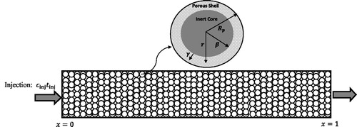
A GRM of liquid chromatography contains two mass balance equations, one is for the total amount of liquid phase in the column and the other one is for the total amount of liquid stored in the solid phase. An isothermal adsorption column packed with inert core particles is considered as shown in Figure 1. Each core-shell particle has three storage regions, i.e. the inert core (impermeable), the pores, and the inner surface. At time zero, a step change in the concentration of an adsorbate is introduced into a flowing stream. The adsorption column is subjected to axial dispersion, film mass transfer resistance and intraparticle diffusion resistance. It is assumed that cored beads have uniform particle size R_p and core size $R_{ \text{core}}$. The inert core cannot be penetrated and there is only diffusion (no convection) in the porous shell. As this study is concerned with the cored particles of arbitrary core radius fraction ${\rho }_{\text{core}}=\frac{R_{ \text{core}}}{R_p}$, it is necessary to allow the core radius to be changed. The column is considered to be isothermal and thermally insulated.

Figure 1. Schematic diagrams of a fixed-bed column packed with inert-core adsorbents.

The differential mass balance equations for a single-solute percolating through a column filled with spherical core beads is given as^[4](1) $${ϵ}_e\frac{\partial c}{\partial t}+(1-{ϵ}_e)(1-{\rho }_{\text{core}}^3)\frac{\partial q^{\text{av}}}{\partial t}+{ϵ}_{e}u\frac{\partial c}{\partial z}={ϵ}_e{D}_z\frac{{\partial }^{2}c}{\partial z^2}$$(1)

In the above equation, c is the concentrations of the solute in the bulk of the fluid, $q^{ \text{av}}$ is the average solute concentration in the particles including the pores, ${ϵ}_e$ is the external porosity, u is the interstitial velocity, D_z represents the axial dispersion coefficient, and t and z denote the time and axial coordinates of the column.

The differential mass balance equation for the solute in the stationary particles can be expressed as^[4](2) $${ϵ}_p\frac{\partial c_p}{\partial t}+(1-{ϵ}_p)\frac{\partial q_p}{\partial t}=\frac{{ϵ}_p{D}_p}{r^2}\frac{\partial }{\partial r}\left(r^2\frac{\partial c_p}{\partial r}\right)+\frac{(1-{ϵ}_p)D_s}{r^2}\frac{\partial }{\partial r}\left(r^2\frac{\partial q_p}{\partial r}\right)$$(2) where c_p denotes the concentration of the solute in the particles pores, q_p is the local concentration of the solute in the shell part of the particle, ${ϵ}_p$ is the internal porosity, $r\in [R_{\text{core}},R_p]$ denotes the radial coordinate (c.f. Figure 1), and D_p and D_s are the constant pore and surface diffusivities, respectively. For fully-porous particles $R_{ \text{core}}=0$, while for core-shell particles $R_{\text{core}}\ne 0$.

The following boundary conditions at r = 0 and r = R_p are assumed for Eq. (2)(2) $${ϵ}_p\frac{\partial c_p}{\partial t}+(1-{ϵ}_p)\frac{\partial q_p}{\partial t}=\frac{{ϵ}_p{D}_p}{r^2}\frac{\partial }{\partial r}\left(r^2\frac{\partial c_p}{\partial r}\right)+\frac{(1-{ϵ}_p)D_s}{r^2}\frac{\partial }{\partial r}\left(r^2\frac{\partial q_p}{\partial r}\right)$$(2) :(3) $${\frac{\partial c_p}{\partial r}|}_{r=R_{\text{core}}}=0,\hspace{1em}{\left[{ϵ}_p{D}_p\frac{\partial c_p}{\partial r}+(1-{ϵ}_p)D_s\frac{\partial q_p}{\partial r}\right]}_{r=R_p}=k_{\text{ext}}(c-{c_p|}_{r=R_p})$$(3)

Eq. (3)(3) $${\frac{\partial c_p}{\partial r}|}_{r=R_{\text{core}}}=0,\hspace{1em}{\left[{ϵ}_p{D}_p\frac{\partial c_p}{\partial r}+(1-{ϵ}_p)D_s\frac{\partial q_p}{\partial r}\right]}_{r=R_p}=k_{\text{ext}}(c-{c_p|}_{r=R_p})$$(3) includes also the additional resistance in the stagnant laminar boundary layer around the particle using the rate constant $k_{\text{ext}}$.

A change in averaged particle concentration in Eq. (1)(1) $${ϵ}_e\frac{\partial c}{\partial t}+(1-{ϵ}_e)(1-{\rho }_{\text{core}}^3)\frac{\partial q^{\text{av}}}{\partial t}+{ϵ}_{e}u\frac{\partial c}{\partial z}={ϵ}_e{D}_z\frac{{\partial }^{2}c}{\partial z^2}$$(1) can be calculated by integrating Eq. (2)(2) $${ϵ}_p\frac{\partial c_p}{\partial t}+(1-{ϵ}_p)\frac{\partial q_p}{\partial t}=\frac{{ϵ}_p{D}_p}{r^2}\frac{\partial }{\partial r}\left(r^2\frac{\partial c_p}{\partial r}\right)+\frac{(1-{ϵ}_p)D_s}{r^2}\frac{\partial }{\partial r}\left(r^2\frac{\partial q_p}{\partial r}\right)$$(2) over the volume, $V_s=\frac{4\pi }{3}(R_p^3-R_{\text{core}}^3)$, of the porous shell. Thus, we obtain^[4](4) $$\begin{array}{c}\frac{\partial q^{\text{av}}}{\partial t}=\frac{1}{V_s}\underset{R_{\text{core}}}{\overset{R_p}{\int }}\left[{ϵ}_p\frac{\partial c_p}{\partial t}+(1-{ϵ}_p)\frac{\partial q_p^{*}}{\partial t}\right]4\pi r^{2}dr\\ =\frac{1}{V_s}\underset{R_{\text{core}}}{\overset{R_p}{\int }}\left[\frac{{ϵ}_p{D}_p}{r^2}\frac{\partial }{\partial r}\left(r^2\frac{\partial c_p}{\partial r}\right)+\frac{(1-{ϵ}_p)D_s}{r^2}\frac{\partial }{\partial r}\left(r^2\frac{\partial q_p}{\partial r}\right)\right]4\pi r^{2}dr\end{array}$$(4)

After integrating the last term in Eq. (4)(4) $$\begin{array}{c}\frac{\partial q^{\text{av}}}{\partial t}=\frac{1}{V_s}\underset{R_{\text{core}}}{\overset{R_p}{\int }}\left[{ϵ}_p\frac{\partial c_p}{\partial t}+(1-{ϵ}_p)\frac{\partial q_p^{*}}{\partial t}\right]4\pi r^{2}dr\\ =\frac{1}{V_s}\underset{R_{\text{core}}}{\overset{R_p}{\int }}\left[\frac{{ϵ}_p{D}_p}{r^2}\frac{\partial }{\partial r}\left(r^2\frac{\partial c_p}{\partial r}\right)+\frac{(1-{ϵ}_p)D_s}{r^2}\frac{\partial }{\partial r}\left(r^2\frac{\partial q_p}{\partial r}\right)\right]4\pi r^{2}dr\end{array}$$(4) and incorporating the boundary condition in Eq. (3)(3) $${\frac{\partial c_p}{\partial r}|}_{r=R_{\text{core}}}=0,\hspace{1em}{\left[{ϵ}_p{D}_p\frac{\partial c_p}{\partial r}+(1-{ϵ}_p)D_s\frac{\partial q_p}{\partial r}\right]}_{r=R_p}=k_{\text{ext}}(c-{c_p|}_{r=R_p})$$(3) , we obtains(5) $$\frac{\partial q^{\text{av}}}{\partial t}=\frac{3}{R_p(1-{\rho }_{\text{core}}^3)}{k}_{ \text{ext}}(c-c_p{|}_{r=R_p})$$(5)

Assuming a permanently established equilibrium between the two phases and considering the linear adsorption isotherm, valid for smaller concentrations, we obtain(6) $$q_p=q_p^{*}=a{c}_p$$(6)

Then, the two transport contributions can be lumped together and can be quantified by a single effective diffusivity coefficient $D_{ \text{eff}}$ and an adjusted equilibrium constant $a^{*}$. After using Eq. (6)(6) $$q_p=q_p^{*}=a{c}_p$$(6) in Eq. (2)(2) $${ϵ}_p\frac{\partial c_p}{\partial t}+(1-{ϵ}_p)\frac{\partial q_p}{\partial t}=\frac{{ϵ}_p{D}_p}{r^2}\frac{\partial }{\partial r}\left(r^2\frac{\partial c_p}{\partial r}\right)+\frac{(1-{ϵ}_p)D_s}{r^2}\frac{\partial }{\partial r}\left(r^2\frac{\partial q_p}{\partial r}\right)$$(2) , we obtain(7) $$a^{*}\frac{\partial c_p}{\partial t}=\frac{D_{\text{eff}}}{r^2}\frac{\partial }{\partial r}\left(r^2\frac{\partial c_p}{\partial r}\right)$$(7) where(8) $$D_{\text{eff}}={ϵ}_p{D}_p+(1-{ϵ}_p)D_{s}a,\hspace{1em}{a}^{*}={ϵ}_p+(1-{ϵ}_p)a$$(8)

Eqs. (1)(1) $${ϵ}_e\frac{\partial c}{\partial t}+(1-{ϵ}_e)(1-{\rho }_{\text{core}}^3)\frac{\partial q^{\text{av}}}{\partial t}+{ϵ}_{e}u\frac{\partial c}{\partial z}={ϵ}_e{D}_z\frac{{\partial }^{2}c}{\partial z^2}$$(1) and (7)(7) $$a^{*}\frac{\partial c_p}{\partial t}=\frac{D_{\text{eff}}}{r^2}\frac{\partial }{\partial r}\left(r^2\frac{\partial c_p}{\partial r}\right)$$(7) are also subjected to the initial and boundary conditions. The initial conditions for an initially equilibrated column are given as(9) $$c(0,z)=c_{\text{init}},\hspace{1em}{c}_p(0,z,r)=c_{\text{init}}$$(9) where $c_{ \text{init}}$ is the spatially uniform initial concentration. For an initially fully regenerated column holds $c_{\text{init}}=0$ which is assumed below. Appropriate inlet and outlet boundary conditions (BCs) are required for Eq. (1)(1) $${ϵ}_e\frac{\partial c}{\partial t}+(1-{ϵ}_e)(1-{\rho }_{\text{core}}^3)\frac{\partial q^{\text{av}}}{\partial t}+{ϵ}_{e}u\frac{\partial c}{\partial z}={ϵ}_e{D}_z\frac{{\partial }^{2}c}{\partial z^2}$$(1) .^[2] In this study, we evaluate a rectangular injection profile and consider the Dirichlet boundary conditions at the column inlet:(10a) $$c{|}_{z=0}=\{\begin{array}{c}{c}_{\text{inj}},\hspace{1em}\text{if} 0<t\le t_{\text{inj}}\hfill \\ 0,\hspace{1em}\hspace{1em}\hspace{1em}\hspace{1em}t>t_{\text{inj}}\hfill \end{array}$$(10a) together with a Neumann boundary condition for a hypothetically infinite column length, $z=\infty$:(10b) $${\frac{\partial c(t,z)}{\partial z}|}_{z\hspace{0.17em}=\hspace{0.17em}\infty }=0$$(10b)

Here, $t_{\text{inj}}$ denotes the time of sample injection. For sufficiently small dispersion coefficients the Dirichlet inlet boundary conditions are well applicable.

Lumped Kinetic Model (LKM)

The LKM can be obtained with some simplifications from the GRM. The model describes the rate of variation of the averaged solute concentration in the stationary phase by assuming a linear driving force originating from the deviation from equilibrium concentration. Thus, it lumps together the two contributions of internal and external mass transport resistances within a mass transfer coefficient $k_{ \text{LKM}}$. In the case of LKM, the second term in Eq. (1)(1) $${ϵ}_e\frac{\partial c}{\partial t}+(1-{ϵ}_e)(1-{\rho }_{\text{core}}^3)\frac{\partial q^{\text{av}}}{\partial t}+{ϵ}_{e}u\frac{\partial c}{\partial z}={ϵ}_e{D}_z\frac{{\partial }^{2}c}{\partial z^2}$$(1) is defined as(11) $$\frac{\partial q^{\text{av}}}{\partial t}=\frac{k_{\text{LKM}}}{1-{ϵ}_e}(q^{\text{av}*}-q^{\text{av}})$$(11) where for a diluted linear system, the equilibrium concentration is $q^{\text{av}*}=\mathit{ac}$. In summary, the LKM contains only two equations as given by Eqs. (1)(1) $${ϵ}_e\frac{\partial c}{\partial t}+(1-{ϵ}_e)(1-{\rho }_{\text{core}}^3)\frac{\partial q^{\text{av}}}{\partial t}+{ϵ}_{e}u\frac{\partial c}{\partial z}={ϵ}_e{D}_z\frac{{\partial }^{2}c}{\partial z^2}$$(1) and (11)(11) $$\frac{\partial q^{\text{av}}}{\partial t}=\frac{k_{\text{LKM}}}{1-{ϵ}_e}(q^{\text{av}*}-q^{\text{av}})$$(11) containing two kinetic parameters D_z and $k_{\text{LKM}}$. The same initial and boundary conditions given by Eqs. (9)(9) $$c(0,z)=c_{\text{init}},\hspace{1em}{c}_p(0,z,r)=c_{\text{init}}$$(9) , (10a)(10a) $$c{|}_{z=0}=\{\begin{array}{c}{c}_{\text{inj}},\hspace{1em}\text{if} 0<t\le t_{\text{inj}}\hfill \\ 0,\hspace{1em}\hspace{1em}\hspace{1em}\hspace{1em}t>t_{\text{inj}}\hfill \end{array}$$(10a) and (10b)(10b) $${\frac{\partial c(t,z)}{\partial z}|}_{z\hspace{0.17em}=\hspace{0.17em}\infty }=0$$(10b) are applied.

Equilibrium Dispersive Model (EDM)

The EDM, which is the most simple one among the models considered, can be obtained from the LKM with one further simplification. It is assumed that there is a permanent equilibrium, i.e. $q^{\text{av}}=q^{\text{av}*}=\mathit{ac}$, which is equivalent to $k_{\text{LKM}}\to \infty$ in the LKM. To compensate this neglect, all mass transfer limitations are lumped into an apparent dispersion coefficient. Under this assumption, Eq. (11)(11) $$\frac{\partial q^{\text{av}}}{\partial t}=\frac{k_{\text{LKM}}}{1-{ϵ}_e}(q^{\text{av}*}-q^{\text{av}})$$(11) is not needed anymore and D_z in Eq. (1)(1) $${ϵ}_e\frac{\partial c}{\partial t}+(1-{ϵ}_e)(1-{\rho }_{\text{core}}^3)\frac{\partial q^{\text{av}}}{\partial t}+{ϵ}_{e}u\frac{\partial c}{\partial z}={ϵ}_e{D}_z\frac{{\partial }^{2}c}{\partial z^2}$$(1) is replaced by a new parameter $D_{\text{app}}$ with $D_{\text{app}}\ge D_z$. Thus, Eq. (1)(1) $${ϵ}_e\frac{\partial c}{\partial t}+(1-{ϵ}_e)(1-{\rho }_{\text{core}}^3)\frac{\partial q^{\text{av}}}{\partial t}+{ϵ}_{e}u\frac{\partial c}{\partial z}={ϵ}_e{D}_z\frac{{\partial }^{2}c}{\partial z^2}$$(1) simplifies to:(12) $$(1+\tilde{a}{F}_e)\frac{\partial c}{\partial t}+u\frac{\partial c}{\partial z}=D_{\text{app}}\frac{{\partial }^{2}c}{\partial z^2}$$(12) where(13) $$F_e=(1-{ϵ}_e)/{ϵ}_e,\hspace{1em}\tilde{a}=a(1-{\rho }_{\text{core}}^3)$$(13)

Again, the same initial and boundary conditions given by Eqs. (9)(9) $$c(0,z)=c_{\text{init}},\hspace{1em}{c}_p(0,z,r)=c_{\text{init}}$$(9) , (10a)(10a) $$c{|}_{z=0}=\{\begin{array}{c}{c}_{\text{inj}},\hspace{1em}\text{if} 0<t\le t_{\text{inj}}\hfill \\ 0,\hspace{1em}\hspace{1em}\hspace{1em}\hspace{1em}t>t_{\text{inj}}\hfill \end{array}$$(10a) and (10b)(10b) $${\frac{\partial c(t,z)}{\partial z}|}_{z\hspace{0.17em}=\hspace{0.17em}\infty }=0$$(10b) are applied.

A more realistic description would require considering further coupling. Indeed, strictly speaking D_z and $k_{\text{ext}}$, but also $k_{\text{LKM}}$ and $D_{\text{app}}$, are functions of the flow-rate of the fluid (i.e. the Reynolds number). There are functional dependencies available in the literature to capture this effect. To take them quantitatively into account would be possible. It would, however, render the analysis much more complicated. Most of the main trends reported in the paper would not change. Thus, for the sake of simplicity we kept these parameters constant.

Analytical Moments of GRM, LKM and EDM

The analytical solutions of linear GRM (Eqs. (1)(1) $${ϵ}_e\frac{\partial c}{\partial t}+(1-{ϵ}_e)(1-{\rho }_{\text{core}}^3)\frac{\partial q^{\text{av}}}{\partial t}+{ϵ}_{e}u\frac{\partial c}{\partial z}={ϵ}_e{D}_z\frac{{\partial }^{2}c}{\partial z^2}$$(1) , (7)(7) $$a^{*}\frac{\partial c_p}{\partial t}=\frac{D_{\text{eff}}}{r^2}\frac{\partial }{\partial r}\left(r^2\frac{\partial c_p}{\partial r}\right)$$(7) ), LKM (Eqs. (1)(1) $${ϵ}_e\frac{\partial c}{\partial t}+(1-{ϵ}_e)(1-{\rho }_{\text{core}}^3)\frac{\partial q^{\text{av}}}{\partial t}+{ϵ}_{e}u\frac{\partial c}{\partial z}={ϵ}_e{D}_z\frac{{\partial }^{2}c}{\partial z^2}$$(1) , (11)(11) $$\frac{\partial q^{\text{av}}}{\partial t}=\frac{k_{\text{LKM}}}{1-{ϵ}_e}(q^{\text{av}*}-q^{\text{av}})$$(11) ) and EDM (Eq. (12)(12) $$(1+\tilde{a}{F}_e)\frac{\partial c}{\partial t}+u\frac{\partial c}{\partial z}=D_{\text{app}}\frac{{\partial }^{2}c}{\partial z^2}$$(12) ) for core-shell particles along with given initial and boundary conditions (c.f. Eqs. (3)(3) $${\frac{\partial c_p}{\partial r}|}_{r=R_{\text{core}}}=0,\hspace{1em}{\left[{ϵ}_p{D}_p\frac{\partial c_p}{\partial r}+(1-{ϵ}_p)D_s\frac{\partial q_p}{\partial r}\right]}_{r=R_p}=k_{\text{ext}}(c-{c_p|}_{r=R_p})$$(3) , (9)(9) $$c(0,z)=c_{\text{init}},\hspace{1em}{c}_p(0,z,r)=c_{\text{init}}$$(9) , (10a)(10a) $$c{|}_{z=0}=\{\begin{array}{c}{c}_{\text{inj}},\hspace{1em}\text{if} 0<t\le t_{\text{inj}}\hfill \\ 0,\hspace{1em}\hspace{1em}\hspace{1em}\hspace{1em}t>t_{\text{inj}}\hfill \end{array}$$(10a) , (10b)(10b) $${\frac{\partial c(t,z)}{\partial z}|}_{z\hspace{0.17em}=\hspace{0.17em}\infty }=0$$(10b) ) are given in the Appendix A exploiting some dimensionless quantities for the kinetic parameters. In order to deduce analytical temporal moments from these solutions, the following moment generating property of the Laplace transform is exploited^[41](14) $${\mu }_n={(-1)}^n\frac{1}{{\mu }_0}\underset{s\to 0}{\lim }\frac{d^n\left(\overline{c}\right(s,x=1\left)\right)}{d{s}^n},\hspace{1em}{\mu }_0=\underset{s\to 0}{\lim }\left(\overline{c}\right(s,x=1\left)\right),\hspace{1em}n=1,2,3,\dots .$$(14)

The corresponding central moments up to order four can be easily obtained as^[42](15) $${\mu }_2^{\prime }={\mu }_2-{\left({\mu }_1\right)}^2,\hspace{1em}{\mu }_3^{\prime }={\mu }_3-3{\mu }_1{\mu }_2+2{\mu }_1{}^3,\hspace{1em}{\mu }_4^{\prime }={\mu }_4-4{\mu }_1{\mu }_3+6{\mu }_1{}^2{\mu }_2-3{\mu }^4$$(15)

It is assumed for the moments derivation that $c_{\text{init}}=0$. Furthermore, results are given only for the column outlet (x = 1).

On using Eqs. (14)(14) $${\mu }_n={(-1)}^n\frac{1}{{\mu }_0}\underset{s\to 0}{\lim }\frac{d^n\left(\overline{c}\right(s,x=1\left)\right)}{d{s}^n},\hspace{1em}{\mu }_0=\underset{s\to 0}{\lim }\left(\overline{c}\right(s,x=1\left)\right),\hspace{1em}n=1,2,3,\dots .$$(14) and (15)(15) $${\mu }_2^{\prime }={\mu }_2-{\left({\mu }_1\right)}^2,\hspace{1em}{\mu }_3^{\prime }={\mu }_3-3{\mu }_1{\mu }_2+2{\mu }_1{}^3,\hspace{1em}{\mu }_4^{\prime }={\mu }_4-4{\mu }_1{\mu }_3+6{\mu }_1{}^2{\mu }_2-3{\mu }^4$$(15) along with the solutions of GRM and LKM (or EDM for $k_{\text{LKM}}\to \infty$ and $D_z=D_{\text{app}}$) in Eq. (A-2)(A-2) $$\overline{c}(s,x)=\frac{(1-e^{-s{\tau }_{\text{inj}}})}{s}\text{exp}\hspace{0.17em}\left[\frac{\mathit{xPe}}{2}\left(1-\sqrt{1+\frac{4\varphi \left(s\right)}{\mathit{Pe}}}\right)\right]$$(A-2) and (A-8)(A-8) $$c(s,x)=\frac{1}{s}\left(c_{\text{inj}}(1-e^{-s{\tau }_{\text{inj}}})-c_{\text{init}}\right)e^{{\lambda }_{1}x}+\frac{c_{\text{init}}}{s}$$(A-8) of Appendix A, we have calculated the first four temporal moments of the considered models which are listed in the Table 1. The zeroth moment μ₀ represents the total mass injected and the first moment μ₁ corresponds to the mean retention time. Kinetic effects are not significant with respect to mean retention time or the first moment. The second central moment $\mu {\prime }_2$, i.e. variance of the elution profile, contains information about the rates of the mass transfer processes in the column. Also, the kinetically controlled third central moment ${\mu }_3^{\prime }$ and the fourth central moment ${\mu }_4^{\prime }$ are helpful to quantify asymmetry and kurtosis of the elution profile.

In chromatography literature the first and second moments are typically exploited to give a number of theoretical plates, $N_t={\mu }_1^2/\mu {\prime }_2$, which is a valuable indicator for the overall column efficiency.^[2]

Relations Between the Kinetic Parameters of Different Models

The analytical solutions and moments of the more comprehensive GRM and of the simpler LKM and EDM for core-shell particles are presented in the Appendix A and Table 1 of this manuscript. In this section, we present relationships between the kinetic parameters of these models by matching their corresponding moments. These relations are helpful to analyze and predict the corresponding concentration profiles.

The linear GRM has a three-level complexity because it contains three essential kinetic parameters D_z, $k_{\text{ext}}$ and $D_{\text{eff}}$. The simpler Linear LKM has a two-level complexity, as it involves only two kinetic parameters D_z and $k_{\text{LKM}}$. On the other hand, the most simpler EDM has a single-level complexity because it contains only one essential kinetic parameter $D_{\text{app}}$.

It is also important to mention again that for evaluating the same injections the zeroth moment, which describes the total mass (volume) of the sample injected to the column, has the same value for all models. Moreover, the first moment, which indicates the mean retention time, can be trivially matched for all models if the overall Henry’s constant $\tilde{a}$ in the LKM and EDM in accordance with the GRM is chosen through the following relation (c.f. Table 1 and Eq. (13)(13) $$F_e=(1-{ϵ}_e)/{ϵ}_e,\hspace{1em}\tilde{a}=a(1-{\rho }_{\text{core}}^3)$$(13) ):(16) $$\tilde{a}={\tilde{a}}^{*}=[{ϵ}_p+(1-{ϵ}_p\left)a\right](1-{\rho }_{\text{core}}^3)$$(16)

There are two general ways to match the elution profiles and second to fourth order central moments of the aforementioned models, as discussed below in Sections 4.1 and 4.2.

Matching the Moments of Low-level Models with Those of High-level Models

In this forward direction, we assume that concentration profiles and moments of the high-level models are known, i.e. they are considered to be “experimental results”, and we try to match them with moments of the simpler models by applying compatible kinetic coefficients. More specifically, there are two possibilities: (a) either try to match the results of simpler EDM and LKM with the provided results of the GRM or (b) match the results of EDM with known results of LKM.

Matching of the Second Moment

The second central moment describes the variance of the elution profile. On comparing the second central moments of the considered models for core shell particles (c.f. Table 1), we obtain the following relations assuming $\tilde{a}={\tilde{a}}^{*}$, i.e. for identical first moments.

Matching a Second Moment of LKM with that of GRM

With the following relation we can match the second central moment of the simpler LKM with that of the comprehensive GRM, while other moments of the GRM will differ from those of the LKM.(17) $$k_{\text{LKM}}={\left[\frac{{\tilde{a}}^{*}}{1-{ϵ}_e}\left(\frac{R_p}{3k_{\text{ext}}}+\frac{R_p^2}{15D_{\text{eff}}}{\rho }_{\text{mod}}\right)\right]}^{-1}$$(17) where ${\rho }_{\text{mod}}$, originally developed by Kaczmarski and Guiochon,^[4] is defined in Table 1. Thus, the above relation and $\tilde{a}={\tilde{a}}^{*}$ ensure that concentration profiles of the LKM and GRM have the same retention times and variances (spreadings) but they may have different asymmetries ($\mu {\prime }_3$) and kurtosis ($\mu {\prime }_4$).

Matching the Second Moment of EDM with that of GRM

Here, we have to use:(18) $$D_{\text{app}}=D_z+\frac{u^2{F}_e{\left({\tilde{a}}^{*}\right)}^2}{{(1+{\tilde{a}}^{*}{F}_e)}^2}\left(\frac{R_p}{3k_{ \text{ext}}}+\frac{R_p^2}{15D_{\text{eff}}}{\rho }_{\text{mod}}\right)$$(18)

Matching the Second Moment of EDM with that of LKM

To match the second central moments of EDM and LKM, one has to fulfill:(19) $$D_{\text{app}}=D_z+\frac{\tilde{a}{u}^2{F}_e^2ϵ}{k_{\text{LKM}}{(1+{\tilde{a}}^{*}{F}_e)}^2}$$(19)

Matching of Third Moment

The third moment, representing asymmetry of the elution profile, provides other matching conditions as given below.

Matching of Third Moment of LKM with that of GRM

On equating the third central moments of LKM and GRM given by Table 1 we obtain from using again $\tilde{a}={\tilde{a}}^{*}$:(20) $$k_{\text{LKM}}=\left[\frac{\alpha +\sqrt{{\alpha }^2+4\beta (\alpha \gamma +\delta )}}{2(\alpha \gamma +\delta )}\right]$$(20) where(21) $$\alpha =\frac{12L{D}_z{\tilde{a}}^{*}{ϵ}_e{F}_e^2(1+{\tilde{a}}^{*}{F}_e)}{u^3}\left[\frac{1}{\mathit{Pe}}(e^{-\mathit{Pe}}-1)+1\right],\hspace{1em}\beta =\frac{6L{\tilde{a}}^{*}{ϵ}_e^2{F}_e^3}{u}$$(21)

(22) $$\gamma =\frac{{\tilde{a}}^{*}}{{ϵ}_e{F}_e}\left(\frac{R_p}{3k_{ \text{ext}}}+\frac{R_p^2}{15D_{\text{eff}}}{\rho }_{\text{mod}}\right)$$(22) (23) $$\delta =\frac{L{\left({\tilde{a}}^{*}\right)}^3{F}_e}{u}\left(\frac{4R_p^4}{105D_{ \text{eff}}^2}{(1-{\rho }_{\text{core}})}^2(1+{\rho }_2)+\frac{4R_p^3}{15k_{\text{ext}}{D}_{\text{eff}}}{\rho }_{\text{mod}}+\frac{2R_p^2}{3k_{\text{ext}}^2}\right)$$(23)

Here, ρ₂ and ${\rho }_{\text{mod}}$ are defined in Table 1.

Matching of Third Moment of EDM with that of GRM

For $\tilde{a}={\tilde{a}}^{*}$ matching of the third moment of EDM with that of GRM requires:(24) $$D_{\text{app}}={\left(\frac{u^5\mu {\prime }_{3, \text{GRM}}(D_z,k_{\text{ext}},D_{\text{eff}},{\rho }_{\text{core}})}{12L{(1+{\tilde{a}}^{*}{F}_e)}^3}\right)}^{\frac{1}{2}}$$(24)

Matching of Third Moment of EDM with that of LKM

To match the third moment of EDM with that of LKM, we have to use:(25) $$\hspace{1em}{D}_{\text{app}}={\left(\frac{u^5\mu {\prime }_{3,\text{LKM}}(D_z,k_{\text{LKM}},{\rho }_{\text{core}})}{12L{(1+\tilde{a}{F}_e)}^3}\right)}^{\frac{1}{2}}$$(25)

In the above two equations $\mu {\prime }_{3,\text{GRM}}$ and $\mu {\prime }_{3,\text{LKM}}$ are the third central moments of GRM and LKM which are assumed to be available either theoretically or experimentally. Relations in Eq. (24)(24) $$D_{\text{app}}={\left(\frac{u^5\mu {\prime }_{3, \text{GRM}}(D_z,k_{\text{ext}},D_{\text{eff}},{\rho }_{\text{core}})}{12L{(1+{\tilde{a}}^{*}{F}_e)}^3}\right)}^{\frac{1}{2}}$$(24) and (25)(25) $$\hspace{1em}{D}_{\text{app}}={\left(\frac{u^5\mu {\prime }_{3,\text{LKM}}(D_z,k_{\text{LKM}},{\rho }_{\text{core}})}{12L{(1+\tilde{a}{F}_e)}^3}\right)}^{\frac{1}{2}}$$(25) guarantee the matching of first and third moments only. All other moments of these models, including the second moment, will differ from each other.

Simultaneously Matching LKM Moments with those of GRM up to Third Order

We might assume that the second and third central moments of GRM are available, may be theoretically or experimentally. Now, we can use the analytical moment expressions of LKM in Table 1 along with Eq. (16)(16) $$\tilde{a}={\tilde{a}}^{*}=[{ϵ}_p+(1-{ϵ}_p\left)a\right](1-{\rho }_{\text{core}}^3)$$(16) to match the first three moments of LKM and GRM. On solving the analytical expressions of second and third central moments of LKM simultaneously for the two unknown parameters D_z and $k_{\text{LKM}}$, we obtain(26) $$k_{\text{LKM}}=\frac{-{\beta }_1\pm \sqrt{{\beta }_1^2+4{\alpha }_1{\gamma }_1}}{2{\alpha }_1},\hspace{1em}{D}_z=\left[\mu {\prime }_{2,\text{GRM}}-\frac{t_{\text{inj}}^2}{12}-\frac{2L{\tilde{a}}^{*}{F}_e^2{ϵ}_e}{u{k}_{\text{LKM}}}\right]\frac{u^3}{2L{(1+{\tilde{a}}^{*}{F}_e)}^2}$$(26) where(27) $${\alpha }_1=\mu {\prime }_{3, \text{GRM}}-\frac{3u}{L(1+{\tilde{a}}^{*}{F}_e)}{\left(\mu {\prime }_{2,\text{GRM}}-\frac{t_{\text{inj}}^2}{12}\right)}^2,\hspace{1em}{\beta }_1=\frac{6{\tilde{a}}^{*}{ϵ}_e{F}_e^2}{1+{\tilde{a}}^{*}{F}_e}\left(\mu {\prime }_{2,\text{GRM}}-\frac{t_{\text{inj}}^2}{12}\right)$$(27)

(28) $${\gamma }_1=\frac{6L{\tilde{a}}^{*}{F}_e^3{ϵ}_e^2}{u}\left[\frac{1+3{\tilde{a}}^{*}{F}_e}{1+{\tilde{a}}^{*}{F}_e}\right]$$(28)

Here, $\mu {\prime }_{2,\text{GRM}}$ and $\mu {\prime }_{3,\text{GRM}}$ are the provided second and third central moments of GRM. With these relations the first three moments of LKM can be perfectly matched with those of GRM. However, the fourth and higher order moments of these models will differ from each other. Due to the involvement of just one single free parameter $D_{\text{app}}$, there is no possibility to match both the second and third moments of EDM with corresponding moments of other models.

Similar procedure can be used to match any other two moments of LKM with those of GRM. For example, one can match the second and fourth order moments or the third and fourth order moments of LKM with those of GRM. Moreover, it is also possible to match any one moment of the EDM with corresponding known moments of the LKM and GRM.

The above estimated parameters and procedure can be used to match the results of low-level models with theoretical results of the high-level models considered to represent the experimental situation. Thus, there is a clear pathway available for rational model complexity reduction.

Matching the Moments of High-level Models with Those of Low-level Models

In this reverse direction, we can assume that concentration profiles and moments of a low-level model are already known and we try to specify free parameters of a high-level model by matching selected moments. For example, we can match the results of LKM and GRM for known parameters of EDM or we can match the results of GRM for known parameters of LKM.

To match the results of LKM with the known results of EDM, we need to estimate two kinetic parameters of the LKM. For this purpose, we can use the analytical expressions of second and third central moments of the LKM and take their Left hand sides as known moments of the EDM. The Newton-Raphson routine can be used to find the roots of resulting two nonlinear equations for two unknowns Pe and ${\kappa }_{ \text{LKM}}$. Similarly, one can select any other combination of two moments of the LKM to find its two unknown parameters.

Moreover, a numerical Newton-Raphson routine can be used to estimate three kinetic parameters of the GRM by utilizing the analytical expressions of its second, third and fourth moments and by providing the corresponding moment expressions and parameters for the EDM or for the LKM.

Numerical Test Problems

In this section, some case studies are presented to analyze and compare concentration profiles and moments of the considered three chromatographic models. The correctness of the matching relations (c.f. Eqs. (17)–(28)) is evaluated based on concentration profiles. In all figures, liquid phase concentration profiles are plotted with respect to the actual time $t=L\tau /u$ at the column outlet (x = 1). Moreover, moments are plotted in the dimensional forms. The dimensionless moments in Table 1 are converted into dimensional forms by simply multiplying μ₀ and μ₁ by L/u and $\mu {\prime }_n$ by ${(L/u)}^n$ for n = 2, 3, 4. Standard parameters used in the test problems are given in Table 2. These model parameters are chosen in accordance with ranges typically encountered in liquid chromatography applications.

Table 2. Parameters assumed in simulations.

Parameters	values
Column length	$L=10\text{cm}$
External porosity	${ϵ}_e=0.4$
Internal porosity	${ϵ}_p=0.333$
Henry’s constant	$a=2.5$
Initial concentration	$c_{\text{init}}=0$
Injected bulk concentration	$c_{\text{inj}}=0.5\mathrm{g}/\mathrm{l}$
Injection time	$t_{\text{inj}}=10$
Core-radius fraction	${\rho }_{\text{core}}=0.5$
Axial dispersion coefficient(GRM, LKM)^a	$D_z=0.02{\text{cm}}^2/\text{min}$
Effective diffusivity coefficient (GRM)	$D_{\text{eff}}={10}^{-6}{\text{cm}}^2/\text{min}$
External mass transfer coefficient (GRM)^a	$k_{\text{ext}}=0.01\text{cm}/\text{min}$
Mass transfer coefficient of LKM^a	$k_{\text{LKM}}=1{\text{min}}^{-1}$
Apparent dispersion coefficient of EDM^a	$D_{\text{app}}=0.02{\text{cm}}^2/\text{min}$

^aAssumed to be the same for different flow rates.

Effect of Core-radius Fraction on the Solutions of Three Models (Non-matching Case)

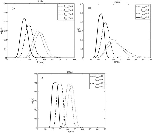
Figure 2 shows a comparison of concentration profiles, obtained from the analytical solutions of investigated models for standard parameters in Table 2, considering different core radius fractions including fully porous beads. Except taking $\tilde{a}={\tilde{a}}^{*}$, kinetic parameters of the models are not calculated through matching relations. Thus, profiles of all the four models have the same retention times but have different band widths and shapes. It can be seen that the effect of ${\rho }_{\text{core}}$ is similar in all cases. As ${\rho }_{\text{core}}$ increases from 0 (fully porous beads) to 0.9 (beads with a very thin shell), the elution profiles sharpens, i.e. column efficiency increases and mean residence time reduces, in other words capacity reduces. The sharpening and the increased symmetry of the peaks in Figure 2 are due to reduced intraparticle diffusional mass transfer resistance. The shorter residence times are due to the loss of binding sites with a larger ${\rho }_{\text{core}}$ value, allowing less interaction between the mobile and the stationary phases for adsorption and desorption. At ${\rho }_{\text{core}}=0.9$ the capacity is very low and profiles are sharper.

Figure 2. Illustration of three models utilizing the non-matched kinetic parameters of Table 2. The effect of ${\rho }_{ \text{core}}$ is shown on the concentration profiles for $u=1 \text{cm}/\text{min}$.

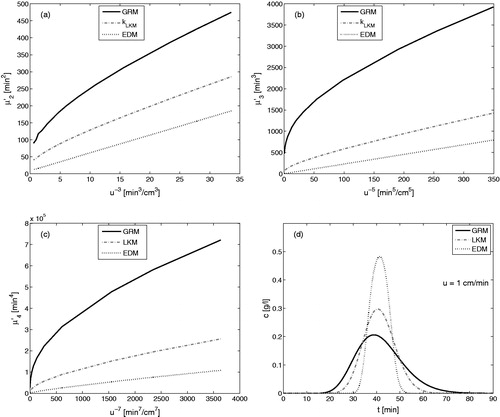
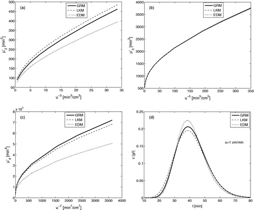
Figure 3 displays moments and concentration profiles of all the four models for a fixed ${\rho }_{\text{core}}=0.5$, for the same adsorption coefficient $\tilde{a}={\tilde{a}}^{*}$, and for the standard parameters listed in the Table 2. It can be observed that all models have different temporal moments and concentration profile. Thus, all the four models may give different results if the matching relations of Section 4 are not fulfilled. These results also endorse the behavior of profiles presents in Figure 2.

Figure 3. Moments and concentration profiles of the considered three models for ${\rho }_{\text{core}}=0.5$ utilizing the non-matched kinetic parameters of Table 2.

Matching the Moments of Low-level Models to Those of High-level Models

Here, we try to either match moments of the LKM and EDM with known moments of the GRM or to mach moments of the EDM with known moments of the LKM.

Matching the Second Central Moments of LKM and EDM with that of GRM

We analyzed the influence of matching relations on moments and concentration profiles of the simpler LKM and EDM, assuming that the results of GRM are already known as given in Figures 2 and 3.

Figure 4 shows the results of all models when relations in Eqs. (17)(17) $$k_{\text{LKM}}={\left[\frac{{\tilde{a}}^{*}}{1-{ϵ}_e}\left(\frac{R_p}{3k_{\text{ext}}}+\frac{R_p^2}{15D_{\text{eff}}}{\rho }_{\text{mod}}\right)\right]}^{-1}$$(17) and (18)(18) $$D_{\text{app}}=D_z+\frac{u^2{F}_e{\left({\tilde{a}}^{*}\right)}^2}{{(1+{\tilde{a}}^{*}{F}_e)}^2}\left(\frac{R_p}{3k_{ \text{ext}}}+\frac{R_p^2}{15D_{\text{eff}}}{\rho }_{\text{mod}}\right)$$(18) are used to match second moment of the simpler models with already known second moment of the GRM. It can be seen that for different flow rates, u, the second central moments of the models are overlapping each other, i.e. they provide the same peak widths. However, these matching relations are not enough to guarantee the matching of higher order moments of the simpler models with those of the GRM. As a result, differences can be seen in the predicted concentration profiles, as they have only the same retention times and variances but have different asymmetries and kurtosis. The concentration profile and higher order moments of the EDM are more deviated from those of the GRM due to more simplifying assumptions (less degrees of freedom) as compared to the LKM.

Figure 4. Matching of the second central moments of simpler models with GRM (c.f. Eqs. (17)–(19)) for ${\rho }_{\text{core}}=0.5$. The kinetic parameters of GRM are taken from Table 2.

Matching the Third Central Moments of LKM and EDM with that of GRM

Figure 5 shows the results of the GRM, LKM, and EDM when matching relations in Eqs. (20)–(25) are used to match the first and third moments. It can be seen that all models have now the same third central moments, i.e. they have the same asymmetries. However, these matching relations are not enough to guarantee the matching of second and fourth moments of the simpler models with those of the GRM. Also, clear differences can be seen in their concentration profiles, especially in their spreading and flatness. It can also be seen that now difference in the fourth moments and concentration profiles of models are much larger as compared to those presented in Figure 4.

Figure 5. Matching of the third central moments of simpler models with GRM (c.f. Eqs. (20)–(24)) for ${\rho }_{\text{core}}=0.5$. The kinetic parameters of GRM are taken from Table 2.

Simultaneously Matching the Moments of LKM with those of GRM up to Third Order

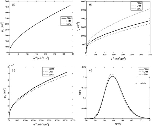
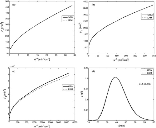
Figure 6 displays the results of GRM and LKM when matching relations in Eqs. (26)(26) $$k_{\text{LKM}}=\frac{-{\beta }_1\pm \sqrt{{\beta }_1^2+4{\alpha }_1{\gamma }_1}}{2{\alpha }_1},\hspace{1em}{D}_z=\left[\mu {\prime }_{2,\text{GRM}}-\frac{t_{\text{inj}}^2}{12}-\frac{2L{\tilde{a}}^{*}{F}_e^2{ϵ}_e}{u{k}_{\text{LKM}}}\right]\frac{u^3}{2L{(1+{\tilde{a}}^{*}{F}_e)}^2}$$(26) and (28)(28) $${\gamma }_1=\frac{6L{\tilde{a}}^{*}{F}_e^3{ϵ}_e^2}{u}\left[\frac{1+3{\tilde{a}}^{*}{F}_e}{1+{\tilde{a}}^{*}{F}_e}\right]$$(28) are used to match their first three moments. It can be seen that both models have the same second and third central moments, i.e. they have now the same variances and asymmetries. However, these matching relations are not enough to guarantee the matching of their fourth (and higher) order moments. It can be observed that both models give almost similar concentration profiles in this case. The EDM involves only one essential kinetic parameter $D_{\text{app}}$, thus, it is not possible to match simultaneously its second and third moments with the corresponding moments of the GRM.

Figure 6. Simultaneously matching the first three moments of simpler models with GRM (c.f. Eqs. (26)–(28)) for ${\rho }_{\text{core}}=0.5$. The kinetic parameters of GRM are taken from Table 2.

Matching the Moments of High-level Models with Those of Low-level Models

Figure 7 shows the results obtained after matching GRM moments to the already known LKM moments as an example. As all the four moments of GRM were used to estimate its kinetic parameters, we can observe a perfect matching of moments and concentration profiles in the Figure 7. In this procedure, we have replaced the left hand sides of GRM moments by known moments of LKM and then found the unknown three kinetic parameters of GRM by using a Newton-Raphson routine. Figure 7(e) displays the absolute errors after comparing the concentration profiles of both LKM and GRM. It can be seen that differences in both profiles are negligible (below $2.5\times {10}^{-5}g/l$) for both flow-rates considered. It can be seen that errors are larger for the higher flow-rate corresponding to the sharper profile.

Figure 7. Matching of GRM moments with the known moments of LKM (${\rho }_{\text{core}}=0$). The kinetic parameters of LKM are taken from Table 2.

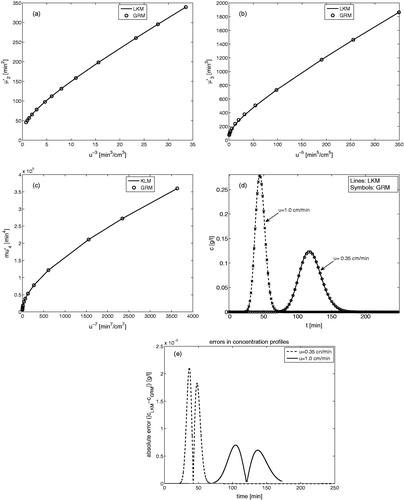
The same procedure was used to match the first four moments of GRM with the provided moments of EDM. Similar trends were found, which are not presented here.

Effect of Core-radius Fraction on Matching of Moments

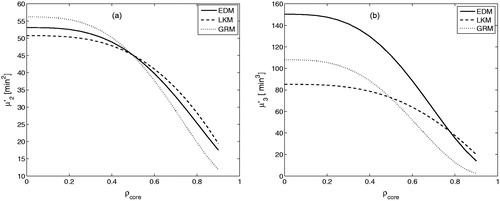
Figure 8 presents the plots of moments for different values of the core-radius fraction ${\rho }_{\text{core}}$. In this case, the LKM moments were assumed to be the provided for a reference value of core-radius fraction (i.e. for ${\rho }_{\text{core}}=0.5$). We then specify the free parameters of the other two models by matching the moments for that particular value of the core-radius fraction. As EDM has only one parameter $D_{\text{app}}$, we were able to match the second moments of both EDM and LKM but not their third moments. On the other hand, we were able to match both the second and third central moments of GRM with those of LKM. The plots of Figure 8 now show that matching at a specific core-radius fraction does not deliver agreement for other values of the core-radius fractions. Thus, care should be taken in matching the moments when the structure of core-beads is changed. Matching of moments obtained for a specific value of ${\rho }_{\text{core}}$ will only hold for that value of ${\rho }_{\text{core}}$ and will not hold when the core-radius fraction is altered.

Figure 8. Effect of ${\rho }_{\text{core}}$ on moments matching (illustrated for $u=1 \text{cm}/\text{min}$). Parameters are selected to match moments for ${\rho }_{\text{core}}=0.5$. The kinetic parameters of LKM are taken from Table 2.

Conclusion

In this article relationships were derived between the essential kinetic parameters of three models for fixed bed columns packed with core-shell particles. These relations were derived by matching the specific analytical expressions describing the temporal moments of the elution profiles for linear isotherms. The Laplace transformation was used as a basic tool to derive the analytical solutions and the first four temporal moments. An efficient and accurate numerical Laplace inversion was applied to get back solutions in the time domain. Several case studies were considered and the analytical solutions and moments of aforementioned models were compared with each other. The results showed that simpler models can be as good as the complex GRM after calculating their kinetic parameters through using matching relations involving essential kinetic parameters of the GRM. The results clearly demonstrate the importance of matching first lower order moments before considering a matching of higher order moments. This concept could be extended and applied also for further refined models of chromatographic columns going beyond the GRM. For practical applications, models capable to well capture the first three moments of a peak are seen as sufficiently accurate. The results presented in this manuscript further showed that an increase in the core radius fraction for cored beads results in shorter residence times and a sharper peaks. Thus, if a column is packed with such beads, the column separation efficiency will increase due to shorter diffusion path lengths, i.e. the peaks will become sharper and narrower. The newly derived moment expressions and the matching relations for the three models considered contain explicitly the core-radius fraction as an additional degree of freedom. Thus, the derived and carefully validated solutions are seen as a useful tool to produce further optimized core-shell particles, to apply them efficiently in chromatographic separation processes, to estimate model parameters from observed experimentally determined moments and to perform in a rational manner a model reduction.

Appendix: Analytical solutions of linear GRM and LKM

Here, we present the analytical solutions of linear GRM and LKM considering core-shell particles.Analytical solution of the linear GRM (already published in our previous article^[23])After introducing the following dimensionless quantities(A-1) $$\begin{array}{c}\tau =\frac{\mathit{ut}}{L},\hspace{1em}x=\frac{z}{L},\hspace{1em}\rho =r/R_p,\hspace{1em}{\rho }_{\text{core}}=R_{\text{core}}/R_p,\\ Pe=\frac{u/L}{D_z/L^2},\hspace{1em}\mathit{Bi}=\frac{k_{\text{ext}}{R}_p}{D_{\text{eff}}},\hspace{1em}\eta =\frac{D_{\text{eff}}L}{R_p^{2}u},\hspace{1em}\xi =3F_e\frac{k_{\text{ext}}}{R_p}\frac{L}{u}\end{array}$$(A-1) and considering Dirichlet boundary conditions (c.f. (10a) and (10b)), the Laplace domain solution is given as^[23](A-2) $$\overline{c}(s,x)=\frac{(1-e^{-s{\tau }_{\text{inj}}})}{s}\text{exp}\hspace{0.17em}\left[\frac{\mathit{xPe}}{2}\left(1-\sqrt{1+\frac{4\varphi \left(s\right)}{\mathit{Pe}}}\right)\right]$$(A-2) where for $\alpha (s)=\frac{a^{*}s}{\eta }$, we have(A-3) $$\varphi \left(s\right)=s+\xi (1-f(s\left)\right),$$(A-3) (A-4) $$f\left(s\right)=\frac{\mathit{Bi}\left[{\rho }_{\text{core}}\right(\sqrt{\alpha \left(s\right)}\left)\coth \right((1-{\rho }_{\text{core}})\sqrt{\alpha \left(s\right)})+1]}{\left(\right(1-{\rho }_{\text{core}})+\mathit{Bi}{\rho }_{\text{core}})\sqrt{\alpha \left(s\right)}[\frac{(\mathit{Bi}+({\rho }_{\text{core}}\alpha \left(s\right)-1\left)\right)}{\left(\right(1-{\rho }_{\text{core}})+\mathit{Bi}{\rho }_{\text{core}})\sqrt{\alpha \left(s\right)}}+\coth ((1-{\rho }_{\text{core}})\sqrt{\alpha \left(s\right)}\left)\right]}$$(A-4)

Moreover, $a^{*}$ and $D_{ \text{eff}}$ are given by Eq. (8)(8) $$D_{\text{eff}}={ϵ}_p{D}_p+(1-{ϵ}_p)D_{s}a,\hspace{1em}{a}^{*}={ϵ}_p+(1-{ϵ}_p)a$$(8) .

7.2 Analytical solution of the linear LKM

After using the dimensionless quantities in Eq. (A-1)(A-1) $$\begin{array}{c}\tau =\frac{\mathit{ut}}{L},\hspace{1em}x=\frac{z}{L},\hspace{1em}\rho =r/R_p,\hspace{1em}{\rho }_{\text{core}}=R_{\text{core}}/R_p,\\ Pe=\frac{u/L}{D_z/L^2},\hspace{1em}\mathit{Bi}=\frac{k_{\text{ext}}{R}_p}{D_{\text{eff}}},\hspace{1em}\eta =\frac{D_{\text{eff}}L}{R_p^{2}u},\hspace{1em}\xi =3F_e\frac{k_{\text{ext}}}{R_p}\frac{L}{u}\end{array}$$(A-1) and the definition(A-5) $${\kappa }_{\text{LKM}}=\frac{k_{\text{LKM}}}{u/L}$$(A-5) the normalized forms of LKM equations (c.f. Eqs. (1)(1) $${ϵ}_e\frac{\partial c}{\partial t}+(1-{ϵ}_e)(1-{\rho }_{\text{core}}^3)\frac{\partial q^{\text{av}}}{\partial t}+{ϵ}_{e}u\frac{\partial c}{\partial z}={ϵ}_e{D}_z\frac{{\partial }^{2}c}{\partial z^2}$$(1) and (11)(11) $$\frac{\partial q^{\text{av}}}{\partial t}=\frac{k_{\text{LKM}}}{1-{ϵ}_e}(q^{\text{av}*}-q^{\text{av}})$$(11) ) are given as(A-6) $$\frac{\partial c}{\partial \tau }+(1-{\rho }_{\text{core}}^3)F_e\frac{\partial q}{\partial \tau }+\frac{\partial c}{\partial x}=\frac{1}{\mathit{Pe}}\frac{{\partial }^{2}c}{\partial x^2}$$(A-6) (A-7) $$\frac{\partial q}{\partial \tau }=\frac{{\kappa }_{\text{LKM}}}{{ϵ}_e{F}_e}\left(\mathit{ac}-q\right)$$(A-7)

By applying the Laplace transformation on Eqs. (A-6)(A-6) $$\frac{\partial c}{\partial \tau }+(1-{\rho }_{\text{core}}^3)F_e\frac{\partial q}{\partial \tau }+\frac{\partial c}{\partial x}=\frac{1}{\mathit{Pe}}\frac{{\partial }^{2}c}{\partial x^2}$$(A-6) and (A-7)(A-7) $$\frac{\partial q}{\partial \tau }=\frac{{\kappa }_{\text{LKM}}}{{ϵ}_e{F}_e}\left(\mathit{ac}-q\right)$$(A-7) and using the initial conditions $c(0,x)=c_{\text{init}}$ and $q(0,x)=q_{\text{init}}^{*}=a{c}_{\text{init}}$, we obtain the following Laplace domain solution^[20,21](A-8) $$c(s,x)=\frac{1}{s}\left(c_{\text{inj}}(1-e^{-s{\tau }_{\text{inj}}})-c_{\text{init}}\right)e^{{\lambda }_{1}x}+\frac{c_{\text{init}}}{s}$$(A-8) where(A-9) $${\lambda }_{1,2}=\frac{\mathit{Pe}}{2}\mp \frac{1}{2}\sqrt{{\left(\mathit{Pe}\right)}^2+4s\mathit{Pe}\left(1+\frac{\tilde{a}{F}_e}{1+\frac{s{ϵ}_e{F}_e}{{\kappa }_{ \text{LKM}}}}\right)}$$(A-9)

Here, ${\tau }_{\text{inj}}=u{t}_{\text{inj}}/L$. An efficient and accurate numerical Laplace inversion algorithm is applied for back transformation of the solution in τ-domain.^[24]

References

- Guiochon, G.; Lin, B. Modeling for Preparative Chromatography; Academic Press: New York, USA, 2003.
- Guiochon, G.; Felinger, A.; Shirazi, D. G.; Katti, A. M. Fundamentals of Preparative and Nonlinear Chromatography; 2nd ed.; Elsevier Academic Press: New York, USA, 2006.
- Li, P.; Xiu, G.; Rodrigues, A. E. Modeling Separation of Proteins by Inert Core Adsorbent in a Batch Adsorber. Chem. Eng. Sci. 2003, 58, 3361–3371. DOI: 10.1016/S0009-2509(03)00217-3.
- Kaczmarski, K.; Guiochon, G. Modeling of the Mass-transfer Kinetics in Chromatographic Columns Packed with Shell and Pellicular Particles. Anal. Chem. 2007, 79, 4648–4656. DOI: 10.1021/ac070209w.
- Horvath, C. G.; Preiss, B. A.; Lipsky, S. R. Fast Liquid Chromatography: An Investigation of Operating Parameters and the Separation of Nucleotides on Pellicular Ion Exchangers. Anal. Chem. 1967, 39, 1422–1428. DOI: 10.1021/ac60256a003.
- Guiochon, G.; Gritti, F. Shell Particles, Trials, Tribulations and Triumphs. J. Chromatogr. A. 2011, 1218, 1915–1938. DOI: 10.1016/j.chroma.2011.01.080.
- Kaczmarsk, K. On the Optimization of the Solid Core Radius of Superficially Porous Particles for Finite Adsorption Rate. J. Chromatogr. A. 2011, 1218, 951–958. DOI: 10.1016/j.chroma.2010.12.093.
- Felinger, A.; Guiochon, G. Comparison of the Kinetic Models of Linear Chromatography. J. Chromatogr. Suppl. 2004, 60, S175–S180.
- Broeckhoven, K.; Cabooter, D.; Desmet, G. Kinetic Performance Comparison of Fully and Superficially Porous Particles with Sizes Ranging between 2.7 μm and 5 μm : Intrinsic Evaluation and Application to a Pharmaceutical Test Compound. J. Pharm. Anal. 2013, 3, 313–323. DOI: 10.1016/j.jpha.2012.12.006.
- Cavazzini, A.; Gritti, F.; Kaczmarski, K.; Marchetti, N.; Guiochon, G. Mass-transfer Kinetics in a Shell Packing Material for Chromatography. Anal. Chem. 2007, 79, 5972–5979. DOI: 10.1021/ac070571a.
- Gu, T.; Liu, M.; Cheng, K.-S. C.; Ramaswamy, S.; Wang, C. A General Rate Model Approach for the Optimization of the Core Radius Fraction for Multicomponent Isocratic Elution in Preparative Nonlinear Liquid Chromatography Using Cored Beads. Chem. Eng. Sci. 2011, 66, 3531–3539. DOI: 10.1016/j.ces.2011.04.021.
- Kahsay, G.; Broeckhoven, K.; Adams, E.; Desmet, G.; Cabooter, D. Kinetic Performance Comparison of Fully and Superficially Porous Particles with a Particle Size of 5 μm: Intrinsic Evaluation and Application to the Impurity Analysis of Griseofulvin. Talanta. 2014, 122, 122–129. DOI: 10.1016/j.talanta.2014.01.050.
- Lambert, N.; Kiss, I.; Felinger, A . Mass-transfer Properties of Insulin on Core-shell and Fully Porous Stationary Phases. J. Chromatogr. A. 2014, 1366, 84–91. DOI: 10.1016/j.chroma.2014.09.025.
- Li, P.; Xiu, G.; Rodrigues, A. E. Analytical Breakthrough Curves for Inert Core Adsorbent with Sorption Kinetics. AIChE J. 2003, 49, 2974–2979. DOI: 10.1002/aic.690491127.
- Li, P.; Xiu, G.; Rodrigues, A. E. Modeling Break Through and Elution Curves in Fixed Bed of Inert Core Adsorbents: Analytical and Approximate Solutions. Chem. Eng. Sci. 2004, 59, 3091–3103. DOI: 10.1016/j.ces.2004.04.034.
- Li, P.; Yu, J.; Xiu, G.; Rodrigues, A. E. A Strategy for Tailored Design of Efficient and Low-pressure Drop Packed Column Chromatography. AIChE J. 2010, 56, 3091–3098. DOI: 10.1002/aic.12218.
- Li, P.; Xiu, G.; Rodrigues, A. E. Modeling Diffusion and Reaction for Inert-Core Catalyst in Batch and Fixed Bed Reactors. Can. J. Chem. Eng. 2019, 97, 217-225. DOI: 10.1002/cjce.23189.
- Gengling, Y.; Zhide, H. Universal Theoretical Moment Expression for Elution and Formal Chromatography of Pellicular Ion Exchange Resins. React. Funct. Polym. 1996, 31, 25–29. DOI: 10.1016/1381-5148(96)00037-5.
- Zhou, X.; Sun, Y.; Liu, Z. Superporous Pellicular Agarose-glass Composite Particle for Protein Adsorption. Biochem. Eng. J. 2007, 34, 99–106. DOI: 10.1016/j.bej.2006.09.018.
- Javeed, S.; Qamar, S.; Ashraf, W.; Seidel-Morgenstern, A.; Warnecke, G. Analysis and Numerical Investigation of Two Dynamic Models for Liquid Chromatography. Chem. Eng. Sci. 2013, 90, 17–31. DOI: 10.1016/j.ces.2012.12.014.
- Qamar, S.; Abbasi, J. N.; Javeed, S.; Shah, M.; Khan, F. U.; Seidel-Morgenstern, A. Analytical Solutions and Moment Analysis of Chromatographic Models for Rectangular Pulse Injections. J. Chromatogr. A. 2013, 1315, 92–106. DOI: 10.1016/j.chroma.2013.09.031.
- Qamar, S.; Abbasi, J. N.; Javeed, S.; Seidel-Morgenstern, A. Analytical Solutions and Moment Analysis of General Rate Model for Linear Liquid Chromatography. Chem. Eng. Sci. 2014, 107, 192–205. DOI: 10.1016/j.ces.2013.12.019.
- Qamar, S.; Abbasi, J. N.; Mehwish, A.; Seidel-Morgenstern, A. Linear General Rate Model of Chromatography for Core-shell Particles: Analytical Solutions and Moment Analysis. Chem. Eng. Sci. 2015, 137, 352–363. DOI: 10.1016/j.ces.2015.06.053.
- Durbin, F. Numerical Inversion of Laplace Transforms: An Efficient Improvement to Dubner and Abate’s Method. Comput. J. 1974, 17, 371–376. DOI: 10.1093/comjnl/17.4.371.
- Rice, R. G.; Do, D. D. Applied Mathematics and Modeling for Chemical Engineers; Wiley-Interscience: New York, USA, 1995.
- Dorota, A.; Kaczmarski, K.; Wojciech, P.; Seidel-Morgenstern, A. Concentration Dependence of Lumped Mass Transfer Coefficients Linear versus Non-linear Chromatography and Isocratic versus Gradient Operation. J. Chromatogr. A. 2003, 1006, 61–76. DOI: 10.1016/S0021-9673(03)00948-8.
- Kubin, M. Beitrag Zur Theorie Der Chromatographie. Collect. Czech. Chem. Commun. 1965, 30, 1104–1118. DOI: 10.1135/cccc19651104.
- Kubin, M. Beitrag Zur Theorie Der Chromatographie II. Einfluss Der Diffusion Ausserhalb Und Der Adsorption Innerhalb Des Sorbens-Korns. Collect. Czech. Chem. Commun. 1965, 30, 2900–2907. DOI: 10.1135/cccc19652900.
- Kucera, E. Contribution to the Theory of Chromatography: Linear Non-equilibrium Elution Chromatography. J. Chromatogr. A. 1965, 19, 237–248. DOI: 10.1016/S0021-9673(01)99457-9.
- Li, P.; Yu, J.; Xiu, G.; Rodrigues, A. E. Perturbation Chromatography with Inert Core Adsorbent: Moment Solution for Two-component Nonlinear Isotherm Adsorption. Chem. Eng. Sci. 2011, 66, 4555–4560. DOI: 10.1016/j.ces.2011.06.016.
- Miyabe, K.; Guiochon, G. Influence of the Modification Conditions of Alkyl Bonded Ligands on the Characteristics of Reversed-phase Liquid Chromatography. J. Chromatogr. A. 2000, 903, 1–12. DOI: 10.1016/S0021-9673(00)00891-8.
- Miyabe, K.; Guiochon, G. Measurement of the Parameters of the Mass Transfer Kinetics in High Performance Liquid Chromatography. J. Sep. Sci. 2003, 26, 155–173. DOI: 10.1002/jssc.200390024.
- Miyabe, K. Surface Diffusion in Reversed-phase Liquid Chromatography Using Silica Gel Stationary Phases of Different C1 and C18 Ligand Densities. J. Chromatogr. A. 2007, 1167, 161–170. DOI: 10.1016/j.chroma.2007.08.045.
- Miyabe, K. Moment Analysis of Chromatographic Behavior in Reversed-phase Liquid Chromatography. J. Sep. Sci. 2009, 32, 757–770. DOI: 10.1002/jssc.200800607.
- Ruthven, D. M. Principles of Adsorption and Adsorption Processes; Wiley-Interscience: New York, USA, 1984.
- Schneider, P.; Smith, J. M. Adsorption Rate Constants from Chromatography. AIChE J. 1968, 14, 762–771. DOI: 10.1002/aic.690140516.
- Suzuki, M. Notes on Determining the Moments of the Impulse Response of the Basic Transformed Equations. J. Chem. Eng. Japan. 1974, 6, 540–543. DOI: 10.1252/jcej.6.540.
- Wolff, H.-J.; Radeke, K.-H.; Gelbin, D. Heat and Mass Transfer in Packed beds-IV Use of Weighted Moments to Determine Axial Dispersion Coefficient. Chem. Eng. Sci. 1979, 34, 101–107. DOI: 10.1016/0009-2509(79)85181-7.
- Wolff, H.-J.; Radeke, K.-H.; Gelbin, D. Weighted Moments and the Pore-diffusion Model. Chem. Eng. Sci. 1980, 35, 1481–1485. DOI: 10.1016/0009-2509(80)85152-9.
- Qamar, S.; Sattar, F. A.; Abbasi, J. N.; Seidel-Morgenstern, A. Numerical Simulation of Nonlinear Chromatography with Core-shell Particles Applying the General Rate Model. Chem. Eng. Sci. 2016, 147, 54–64. DOI: 10.1016/j.ces.2016.03.027.
- Van der Laan, T. Letter to the Editors on Notes on the Diffusion Type Model for the Longitudinal Mixing in Flow. Chem. Eng. Sci. 1958, 7, 187–191.
- Papoulis, A. Probability, Random Variables, and Stochastic Processes, 2nd ed.; McGraw-Hill: New York, USA, 1984; p. 146.