The Economic Impact of Extreme Cyber Risk Scenarios

Abstract

Numerous industry studies discuss the economic effects of potentially extreme cyber incidents, with considerable variation in the applied methodology and estimated costs. We implement a dynamic inoperability input–output model that allows a consistent analysis and comparison of the economic impacts resulting from six widely discussed cyber risk scenarios. Our model accounts for the frequently omitted qualitative context of the scenarios to be considered as part of the economic projection. Overall, our loss estimations remain in an insurable range from US$0.7 to 35 billion. To our knowledge, this is the first effort to develop a standardized evaluation framework that allows for a consistent assessment of cyber risk scenarios, thereby enabling comparability.

1. MOTIVATION AND AIM

The transition of society to a global knowledge-based economy, the increasing dependency on the information technology (IT) sector, and the integration of digital technologies into almost any sphere of life expose organizations to cyber risks. One example of the potential drastic consequences was when the 2017 WannaCry ransomware crippled health care institutions and many other organizations around the world, leading to economic losses estimated at US$8 billion (Weintraub and Borenstein 2017; Parenty and Domet 2019). In 2020 the overall economic costs of cybercrime are estimated to be in the area of US$1000 billion per year (Smith, Lostri, and Lewis 2021, 3), up from 600 billion US$per year in 2018 (Lewis 2018, 4). COVID-19 and the increasing use of digital technologies in the postpandemic world have further increased the economic relevance of cyber risks (see, e.g., Chigada and Madzinga 2021; Lallie et al. 2021; Li and Liu 2021). However, due to the limited availability of historical data, which is partially attributable to disincentives for cyber incident reporting and disclosing (see, e.g., Lagazio et al. 2014), cyber risk cost estimates (which encompass far more than cybercrime) are scarce and vary considerably across studies. Furthermore, the inherent variability and multidisciplinary context of study across cyber risks limits the use of historical data for cyber risk analysis; historical events are not necessarily a useful indicator for future events (see, e.g., Falco et al. 2019).

As an alternative and to raise the awareness among policymakers, media, the public, and executives, various scenarios have been proposed in the applied literature and in industry studies (see, e.g., Kelly et al. 2016; Risk Management Solutions, Inc. 2016; Ruffle et al. 2014). These worst-case scenarios include various incidents that lead to a disruption of critical infrastructure and thus to economic losses. One often-discussed aspect in this context is the monocultures in soft- and hardware markets that result in potential loss accumulation in the event of a cyber incident (see, e.g., Eling and Schnell 2020). The projected economic effects of the scenarios show some extreme variations, ranging from 0.2% to 2% of the gross domestic product (GDP) in the year of the event. However, as the studies lack common approaches, objectives, and thematic areas, the comparability of the scenarios and a comparative economic impact analysis are only possible to a limited extent (see e.g., Nikolakopoulos et al. 2016). All this leaves managers and policymakers with a vague idea on potential frequency and severity of extreme cyber risks, resulting in vague risk management strategies as well.

We develop a methodology that allows a consistent economic impact analysis resulting from different cyber risk scenarios. To achieve this, we review and evaluate six widely discussed cyber risk scenarios and filter the specific characteristics of each scenario. A standardized framework for the quantification of economic losses due to cyber risks is then proposed to assess the costs of historical and future incidents, which can be applied on a macroeconomic and microbusiness level. This allows organizations to determine the optimal amount spent on information security and to measure its effectiveness in a consistent and replicable way. To our knowledge, this is the first effort to consistently analyze the economic impact of various cyber risk scenarios proposed in the applied literature.¹ The consistent evaluation framework allows comparability and scalability for potential future scenarios. The findings are useful for practitioners, policymakers, and regulators in improving the understanding of this new type of risk.

Applying our methodology to six well-known scenarios yields economic loss estimations for the United States ranging from US$0.7 to 35 billion. The calculated losses fall within the realm of insurability. This is important because policymakers can use this information to assess for which cyber risk scenarios there may be a need for government backstops and other market-intervening tools that mitigate catastrophic losses. The two most extreme cases are a health sector and hospitals scenario and a cross-sector attack scenario with loss estimations of US$28 and 35 billion. These numbers are in the top 10 of the largest loss events in history, but significantly smaller than the largest catastrophic events, which are the Japanese tsunami in 2011 (US$210 billion) and Hurricane Katrina in 2005 (US$125 billion), losses that could be covered by insurance and reinsurance companies in the past.² We also note that even the largest loss estimates are only 0.17% of the U.S. GDP (US$35 billion versus $20.5 trillion; World Bank 2019), which provides some perspective for extreme loss estimates documented in some industry studies (up to 2% of GDP). Although the loss estimators derived in our study are large, the overall picture gives positive signals on the capacity of insurance and reinsurance companies to provide coverage also for extreme cyber loss scenarios.

In the following, we first introduce our methodology. Then we identify relevant cyber risk scenarios and measure their potential economic impact. Finally, we present our conclusions.

2. DEFINITIONS AND LITERATURE REVIEW

2.1. Cyber Risk

An unambiguous definition of cyber risk does not exist. Cyber risk includes identity theft, business interruption, reputational damage, theft of customer records, and data recovery costs as well as litigation costs (European Union Agency for Network and Information Security 2018; National Association of Insurance Commissioners 2019). Focusing on the operational side, cyber security risks can be defined as “operational risks to information and technology assets that have consequences affecting the confidentiality, availability or integrity of information or information systems” (Cebula et al. 2014). Such a broad definition is justified as various and evolving causes constitute the basis of cyber risk.

Cyber risks can be classified by activity (e.g., criminal and noncriminal), type of attack (e.g., distributed denial of service attack, malware), and source of attack, also called threat actor (e.g., terrorists, criminals, and governments).³ Unlike other risks typically covered by insurers, cyber risks are characterized by a high correlation and the general difficulty of verifying the loss to the insurance company (Öğüt et al. 2011). The high correlation is attributable on the one hand to global interconnectedness and on the other hand to economies of scale associated with the development of IT systems (see Baldwin et al. 2017).

As modern technology is being integrated into complex sociotechnological networks in critical infrastructure⁴ of sectors such as energy, telecommunication, and banking, cyber risk is becoming an increasing threat. Due to the growing interdependency within and between sectors, a failure in critical infrastructure caused by a cyberattack could cascade across national and sectoral boundaries, potentially resulting in catastrophic consequences (Pescaroli and Alexander 2016; Zio 2016).

2.2. Scenario Analysis

Scenarios are “plausible descriptions of how the future may develop based on a coherent and internally consistent set of assumptions” (Nakicenovic and Swart 2000). Scenarios in this sense are neither predictions nor forecasts but structured accounts of possible future states (Peterson et al. 2003). Scenario analysis is a method of strategic planning and decision making applied in politics, science, and business. A scenario analysis typically consists of five phases: scenario definition, scenario construction, scenario analysis, scenario assessment, and risk management (Mahmoud et al. 2009). A scenario must satisfy five conditions simultaneously: pertinence, coherence, likelihood, importance, and transparency (Durance and Godet 2010). As historical claims experience may not be a good predictor of future costs of cyber incidents, scenarios might provide a remedy.

Cyber events are often analyzed in scenarios (see, e.g., Lloyd’s 2015; Ruffle et al. 2014). We define cyber risk scenarios as alternative, dynamic stories that capture key ingredients of the uncertainty regarding devastating cyber incidents, typically leading to accumulation risks (i.e., widespread and correlated losses). Scenario analysis thereby facilitates the analysis of the likelihood and consequences of the respective scenarios. Cyber risk scenarios are often published in the form of fictional narratives with qualitative descriptions (see, e.g., Risk Management Solutions, Inc. 2016; World Economic Forum 2014). In most quantitative assessments of economic losses resulting from cyberattacks, the context of these scenarios is not considered. The method applied in this article, however, attempts to capture the context of economic loss scenarios using sensitivity analysis to account for the uncertain and fuzzy nature of the parameters used within the scenarios. This is accomplished by deriving parameters from qualitative scenario descriptions, a critical determinant in establishing comparability across scenarios.

Additionally, a consistent typology and classification of the scenarios proposed in the academic literature and practitioner case studies has not yet been established.⁵ Comparing and analyzing different cyber risk scenarios is difficult and is further complicated by the absence of a uniform framework for scenario development. This article describes a standardized and consistent typology and method for the classification of cyber risk scenarios.

2.3. Economic Impact Analysis

The analysis of the economic impacts of cyber risk scenarios has received only limited attention to date in the academic literature compared to the insurability of cyber exposures (see, e.g., Biener et al. 2015; Marotta et al. 2017; Romanosky 2016; Wang 2019). This is mainly attributable to the limited data available on historical cyber incidents and the absence of a standardized methodology for scenario development and impact analysis. The academic literature is outnumbered by a wide array of practitioner case studies (see, e.g., Institute and Faculty of Actuaries 2018; Lloyd’s 2015; Risk Management Solutions, Inc. 2016). They do, however, usually concentrate on one or a few scenarios and do not propose a consistent analytical framework for the assessment of the respective economic impacts. Additionally, the estimated direct and systemic costs⁶ of cyber incidents vary significantly from one study to another and the explanations on the derivation of the estimates are generally not fully transparent.

The RAND Corporation addresses the lack of transparency in methodologies, assumptions, and data in its attempt to develop a transparent methodology for estimating global costs of cyber risk (see Dreyer et al. 2018). In contrast to Dreyer et al. (2018), the focus of this article lies on the provision of a unified language for describing cyber risk scenarios, and comparing their impact using a standardized, replicable, and comparably simple framework. Additionally, our methodology allows the modeling of economic impacts of cyber events caused by untraditional means (e.g., a solar storm); Dreyer et al. (2018) emphasize that the resulting economic losses are highly sensitive to input parameters.⁷ To counteract this, our methodology is limited to only two input parameters. The paper closest to our analysis is Bounfour et al. (2018), which uses the dynamic input–output inoperability model to analyze the impact of cyberattacks on the telecommunications and finance sector. In distinction to Bounfour et al. (2018), this article examines the impact of six cyber risk scenarios that have already been discussed in the literature and values for inoperability and recovery time based on this literature (i.e. historical data and expert opinions), rather than assumptions that are not further justified or motivated. Additionally, the study at hand accounts for the qualitative context of specific cyber risk scenarios. To our knowledge, no extant study takes a holistic approach to combine and analyze the various scenarios proposed in the literature in terms of their economic impact.

Outside the cyber risk domain, several models for disaster impact analysis have been proposed (see, e.g., Rose et al. 2016; Wei et al. 2018). Economic losses resulting from disasters have been forecasted with three models: econometric models,⁸ input–output models,⁹ and computable general equilibrium models¹⁰ (Avelino and Hewings 2017; Menoni et al. 2017). The latter two are the most frequently applied and best documented approaches in disaster impact analysis (Koks and Thissen 2016).

The rationale for using one of the already-mentioned models is that cyber incidents induce complex economy-wide and international effects. Modeling helps to calculate the damage caused by historical attacks, to predict the impact of cyber risks that have not yet occurred, and to improve decision-making processes. In addition, these models enable a better understanding of cyber risks and the development of more effective cyber insurance to hedge the economic impact of the risk. In contrast to proprietary, company-specific cyber risk models, the mentioned variants enable the analysis of large-area cyber risks with potential cumulative effects. As affected companies tend to not report cyber incidents, only limited information on cyber risk is publicly available. With the help of the macroeconomic models, the effects of different cyber risk scenarios can be analyzed without having to resort to aggregated data from historical events. A further advantage is the flexibility of the models, which makes it possible to estimate the damage caused by new cyber risk scenarios. The well-documented application of the models also enables other researchers to analyze the effects of their own cyber risk scenarios.

Since econometric models require the availability of consistent time-series data over a reasonably long period of time, this methodology is not suitable for the analysis of ever-changing and novel cyber risks. A projection of the past is very likely not appropriate for estimating the potential economic losses resulting from cyberattacks. Furthermore, in contrast to input–output and computable general equilibrium models, econometric models encounter difficulties in distinguishing between direct and indirect effects (Rose 2004).

Computable general equilibrium models are capable of quantifying the far-reaching ramifications of disruptions to the economic system. Unfortunately, the nonlinearity of computable general equilibrium models requires complex solution algorithms (West 1995). A further barrier to the use of the computable general equilibrium model is that it requires a full optimization. The advantages and disadvantages as well as various papers in which the three aforementioned models were applied are summarized in Appendix A (Table 6).

We apply the input–output model, a transparent methodology allowing other researchers to replicate the results and to analyze their own cyber risk scenarios. As the analyzed scenarios are only vaguely defined, more sophisticated models (such as the computable general equilibrium model) may provide similar results without adding additional value, while simultaneously increasing complexity and reducing transparency and replicability. Furthermore, the input–output model allows one to explicitly reflect the economic interdependencies between different sectors, including higher order effects, which might be important considering the diverse implications of cyber risk events. In addition, the input–output model is more appropriate for analyzing the effects of short-term disturbances (which cyberattacks usually are), which is in contrast to computable general equilibrium models that analyze long-term effects by considering price adjustments. Additionally, the economic consequences of natural disasters and human-made hazards have recently been mainly analyzed using the input–output model or extensions thereof. The application of the input–output model thus allows a holistic estimation of economic losses resulting from cyberattacks and accounts for different recovery times.

3. METHODOLOGY

3.1. Leontief Input–Output Model

The Leontief input–output model describes the equilibrium behavior of regional and national economies.¹¹ The areas of application of input–output analysis today extend considerably further than the original use for quantifying the extent of economic shifts (e.g., changes in consumption). The input–output model helps to analyze the effects of disruptions on the economy, which consist of a multitude of interdependent sectors. Since each sector is dependent on input factors provided by other industries, interdependencies arise. The model also includes foreign trade (i.e., import and export) and consumption by households. The basic function of the original input–output model is as follows (Santos 2006; Lian and Haimes 2006): (1) $$\mathit{x}=\mathit{Ax}+\mathit{c}\stackrel{}{\iff }\left\{x_i=\sum _j{a}_{ij}{x}_j+c_i\right\}\forall i.$$(1) where $x_i$ represents the total production output of sector $i,$ $a_{ij}$ the Leontief technical coefficient that indicates the ratio of the input from sector $i$ to sector $j$ with respect to the overall production requirements of sector $j,$ and $c_i$ the final demand of the $i$ th sector, defined as the portion of sector $i$’s total output for final consumption by end-users.

3.2. Inoperability Input–Output Model

The demand-based input–output inoperability model is an extension of the traditional Leontief input–output model introduced by Haimes and Jiang (2001). Both the inoperability input–output model and the traditional Leontief input–output model are based on the same data set and are deterministic linear equilibrium models (Santos 2006). However, there are several theoretical and practical differences. Instead of the technical coefficient matrix, the inoperability input–output model makes use of an interdependency matrix (Jung et al. 2009).

The inoperability input–output model allows analyzing how the inoperability of a given economic sector (i.e., the inability to perfectly fulfil its function¹²) affects the overall economy and how the inoperability is amplified and spread through interdependencies (Panzieri and Setola 2008). Through its ability to model ripple effects, the inoperability input–output model has aroused the interest of both researchers and policymakers. In the inoperability input–output model the inoperability vector is formulated as (2) $$\mathit{q}={\mathit{A}}^{\mathrm{*}}\mathit{q}+{\mathit{c}}^{\mathrm{*}}={[\mathit{I}-{\mathit{A}}^{\mathrm{*}}]}^{-1}{\mathit{c}}^{\mathrm{*}}$$(2) where $\mathit{q}$ represents the demand-based inoperability vector, ${\mathit{A}}^{\mathit{*}}$ the demand-based interdependency matrix derived from the technical coefficient matrix $\mathit{A},$ $\mathit{I}$ the identity matrix, and ${\mathit{c}}^{\mathit{*}}$ the demand-based perturbation vector, whereby¹³ (3) $$\mathit{q}={\widehat{\overline{\mathit{x}}}}^{-1}\delta \mathit{x}$$(3) (4) $${\mathit{A}}^{\mathbf{*}}={\widehat{\overline{\mathit{x}}}}^{-1}\mathit{A}\widehat{\overline{\mathit{x}}}$$(4) (5) $${\mathit{c}}^{\mathbf{*}}={\widehat{\overline{\mathit{x}}}}^{-1}\delta \mathit{c}$$(5) (6) $$\partial \mathit{x}=\overline{\mathit{x}}-\tilde{\mathit{x}}$$(6) (7) $$\partial \mathit{c}=\overline{\mathit{c}}-\tilde{\mathit{c}},$$(7) where $\widehat{\overline{\mathit{x}}}$ is the diagonal matrix generated by the vector $\overline{\mathit{x}}$ (which is the baseline industry total production vector), $\tilde{\mathit{x}}$ is the degraded industry total production vector,¹⁴ $\overline{\mathit{c}}$ is the baseline final uses vector, and $\tilde{\mathit{c}}$ is the degraded final uses vector. The elements of matrix ${\mathit{A}}^{\mathit{*}}$ are defined as $a_{ij}^{*}=a_{ij}\frac{x_j}{x_i},$ where $x_i$ and $x_j$ are the outputs of sectors $i$ and $j,$ respectively, and $a_{ij}$ corresponds to the elements of the original technical coefficient matrix $A$ (Ali and Santos 2014).

The inoperability input–output model was extended to the dynamic inoperability input–output model by Haimes et al. (2005). This method incorporates time varying features of (in)operability and the discrete-time¹⁵ postshock resilience capacity of a sector and is defined as follows: (8) $$\mathit{q}(t+1)={\mathit{KA}}^{\mathbf{*}}\mathit{q}\left(t\right)+\mathit{K}{\mathit{c}}^{\mathbf{*}}\left(t\right)+\left(\mathit{I}-\mathit{K}\right)\mathit{q}\left(t\right)$$(8) where $\mathit{q}(t)$ represents the inoperability vector at time $t,$ $\mathit{K}$ the sectoral resilience matrix, ${\mathit{A}}^{\mathit{*}}$ the interdependency matrix derived from the input–output matrix, ${\mathit{c}}^{\mathit{*}}(t)$ the perturbation vector at time $t,$ and $\mathit{I}$ the identity matrix. The initial inoperability value of a particular sector can take any value between zero and one (i.e., $0<q_i(0)<1$). It can be determined using various methods. The values of the initial inoperability in the different cyber risk scenarios were either simply assumed or evaluated by subject-matter experts. The resilience factor $k_i$ of a particular sector $i$ depicts its recovery rate from the external shock and the resulting inoperability. It is defined as follows (Lian and Haimes 2006): (9) $$k_i=\frac{ln\left[\frac{q_i\left(0\right)}{q_i\left(T\right)}\right]}{T_i}\mathrm{*}\left(\frac{1}{1-a_{ii}^{\mathrm{*}}}\right)$$(9) where $T_i$ represents the recovery time of sector $i$¹⁶, and $a_{ii}^{*}$ the technical coefficient from the input–output matrix. Resilience is defined as the ability or capability of a system to absorb or cushion against damage or loss (Holling 1973). The recovery period $T$ is the time a sector requires to achieve an acceptable operability level in comparison to the precatastrophe condition. It can be determined using historical observations or expert judgment (Ali and Santos 2014). Since historical data on cyberattacks are very scarce, the cyber risk scenarios are based on expert opinions in this respect. Following the assumption taken by Ali and Santos (2015), we assume that the inoperability at $T$ corresponds to the state when all sectors have recovered to 1% of their initial inoperability values (i.e., $q_i\left(T\right)=0.01q_i(0)$). The ratio of the initial inoperability with respect to the inoperability at $T$ is as follows: (10) $$\frac{q_i\left(0\right)}{q_i\left(T\right)}=100$$(10)

The actual recovery rate $k_i$ of the $i$ th sector is therefore driven by its own recovery rate as well as its interdependence with the other sectors. The term $1-a_{ii}^{*}$ is defined as the interdependency index of sector $i,$ denoted as ${\theta }_i:$ (11) $${\theta }_i=1-a_{ii}^{\mathrm{*}}$$(11)

The degree of interdependency between two sectors is characterized by the interdependency ratio, denoted as ${\rho }_{ij},$ and is calculated as follows: (12) $${\rho }_{ij}=\frac{{\theta }_i}{{\theta }_j}=\frac{1-a_{ii}^{\mathrm{*}}}{1-a_{jj}^{\mathrm{*}}}$$(12)

For those sectors that are not directly affected by the cyberattack, it is assumed that their production will adapt quickly. Therefore, their industry resilience coefficient $k_i$ is set to 1.

The inoperability values are calculated from the initial inoperability vector $\mathit{q}(0).$ The shape of the inoperability curves is the result of multiple iterations of Equation (8)(8) $$\mathit{q}(t+1)={\mathit{KA}}^{\mathbf{*}}\mathit{q}\left(t\right)+\mathit{K}{\mathit{c}}^{\mathbf{*}}\left(t\right)+\left(\mathit{I}-\mathit{K}\right)\mathit{q}\left(t\right)$$(8) . Since the inoperability of one sector is influenced by that of the other sectors, the inoperability curves can take various shapes (see, e.g., Figure 2). Depending on the affected sectors, the interdependency matrix, and the resilience matrix, inoperability decreases more slowly or more quickly. The recovery curves (i.e., the inverse of the inoperability curve) can take either a linear, trigonometric, or exponential shape (Cimellaro et al. 2010). The exponential recovery function is most likely for the scenarios under consideration since the response to the cyberattack is driven by a high initial effort and inflow of resources to address the problem, while the rapidity of recovery decreases as the process draws to a close where only minor modifications are needed to address bugs. Conversely, this implies that the inoperability curves have a convex shape with a decreasing slope.

The expected value of the total economic loss for a particular cyber risk scenario is calculated as (Lian et al. 2007) (13) $${E[\mathit{Q}}_{\mathit{s}}]=\mathit{diag}(\mathit{x}\left){\left(\mathit{I}-{\mathit{A}}^{\mathbf{*}}\right)}^{-1}{E\left[\mathit{K}\right]}^{-1}\mathit{q}\right(0)$$(13) where ${E[\mathit{Q}}_{\mathit{s}}]$ represents the expected value of the total economic loss in cyber risk scenario $s$ and $\mathit{x}$ represents the nominal output vector of the sectors for a given time period.

For the analysis of the different cyber risk scenarios, different minimum and maximum values for the recovery time and the inoperability were estimated. This approach allows the sensitivity of the results to be presented and to account for the fuzzy nature of the input values. There are more complex methodological approaches, such as the fuzzy dynamic input–output inoperability model by Panzieri and Setola (2008), in which the inoperability of each sector and the dependency coefficients are expressed as fuzzy numbers. Although these are methodologically interesting, we decided to account for the fuzzy nature in a simple minimum/maximum setup that requires no further assumptions. Given the scarcity of data and the various assumptions already needed to estimate the simple input–output model presented here, the additional value of a more complex model seems rather limited.

3.3. Data Sources for the Analysis of Economic Disruptions

We build our model on the harmonized national input–output transaction tables provided by the Organization for Economic Cooperation and Development (OECD 2018). The OECD publishes a set of yearly input–output table combinations, which are based on official and publicly available data from statistical institutions, thus ensuring a high quality of the data and transparency. It presents matrices of interindustrial flows of goods and services (domestically produced and imported) for all members of the OECD and 28 nonmember states (including all G20 countries) covering the years 2005 to 2015. The included sectors are summarized in Appendix B.

Table 1 illustrates a schematic representation of a national input–output table. While the columns contain information on the production processes, the rows indicate the distribution of the outputs. Naturally, the total use of an industry is equal to the gross output of that industry.

TABLE 1 Schematic Representation of an Input–Output Transaction Table (Miller and Blair 2009)

		Producers as consumers								Final demand
		Agriculture	Mining	Construction	Manufacturing.	Trade	Transportation	Services	Other industry	Personal consumption expenditures	Gross private domestic investment	Govt. purchases of goods & services	Net exports of goods & services
Producers	Agriculture
	Mining
	Construction
	Manufacturing
	Trade
	Transportation
	Services
	Other industry
Value added	Employees	Employee compensation								Gross domestic product
	Business owners and capital	Profit-type income and capital consumption allowances
	Government	Indirect business taxes

Two fundamental problems complicate the economic impact analysis of different cyber risk scenarios: the scarcity of historical data on cyber incidents and the lack of a universal standardized framework for assessment. As a result, we resort to a minimum/maximum setup. The cyber risks scenarios are assessed by a literature review.

4. CYBER RISK SCENARIOS

The threats posed by cyberattacks to different industries can take various forms, origins, and degrees of sophistication. Even though natural hazards such as earthquakes and flooding can lead to (physical) IT disruptions, the most probable threats are caused by human-made actions (Ali and Santos 2014). Cyberattacks are executed by politically, economically, or religiously motivated state-sponsored attackers, criminals, hackers, or terrorists (Dejung 2017). The different types of cyberattacks include malware, insider attacks, spam, distributed-denial-of-service attacks, and physical destruction of IT systems (Eling and Schnell 2016). Cyber risk scenarios are used to present the worst possible cyberattacks in a linguistically appealing way. We have selected six cyber risk scenarios that cover the most significant cyberattack threats:

1. An extortion of supervisory control and data acquisition networks.^17,18

2. A cloud service provider failure.¹⁹

3. A cyberattack on the health sector and hospitals.²⁰

4. A compromise of municipal services.²¹

5. An impairment of Internet telecommunications.²²

6. A strategic cross-sector IT failure.²³

These scenarios all exhibit a high potential for cumulative damage, which can extend across different sectors within a country as well as across countries. Furthermore, the scenarios cover a broad spectrum of potential cyberattacks.²⁴ Table 2 contains the classification of the scenarios according to the Computer and Network Incident Taxonomy presented by Howard (1997; 2015; see Appendix C).

TABLE 2 Analyzed Cyberattack Scenarios Classified According to the Computer and Network Incident Taxonomy

Scenario	Attackers	Tool	Vulnerability	Action	Target	Unauthorized result	Objectives
1)	Hackers, terrorists	User commands	Design vulnerability	Delete	Network	Denial of service	Political gain, damage
2)	Professional criminals	Toolkit	Implementation vulnerability	Authenticate	Internetwork	Denial of service	Financial gain
3)	Hackers, terrorists, professional criminals	Script or program	Design vulnerability	Delete	Network	Denial of service	Financial gain, political gain, damage
4)	Hackers, terrorists	Autonomous agent	Configuration vulnerability	Authenticate	Data, network	Denial of service	Financial gain, political gain
5)	Professional criminals	Autonomous agent	Design vulnerability	Modify	Component	Denial of service	Financial gain, political gain, damage
6)	Professional criminals	Autonomous agent	Design vulnerability	Delete	Network	Denial of service	Financial gain

Table 3 contains the selected scenarios and the parameters used for the input–output analysis. A comprehensive summary of the scenarios according to the cyberattack anatomy proposed by Falco et al. (2018), including the estimated frequency and examples of comparable cyberattacks, is included in Table 9 (columns 5 to 8) in Appendix D. The affected sectors in Table 3 are the directly affected sectors; indirect effects on other sectors are modeled in the input–output analysis. We note that all parameters used for the input–output analysis are taken from the respective studies with two exceptions mentioned below the table. We see the combination of the qualitative categorization of cyber risk scenarios using a standardized taxonomy and the quantitative estimation of economic losses (presented in the following section) as major value add. When decision makers are confronted with new scenarios, they can use our results to qualitatively assess how the new scenarios fit into our scenario framework and quantitatively arrive at a rough estimate of its economic impact.

TABLE 3 Summary of the Scenarios and the Respective Input Parameters for the Input–Output Analysis

Scenario	Risk factor	Affected sectors	Initial inoperability	Recovery time
1)	Supervisory control and data acquisition network/industrial control system extortion	D01T03, D10T12, D31T33, D35T39, D41T43, D49T53, D86T88	0.05–0.15*	21 days
2)	Cloud service failure	D62T63*	0.27	1–7 days
3)	Health sector and hospitals	D86T88	0.10–1.00	14–21 days
4)	Municipal services	D84	1.00	5 days
5)	Telecommunication	D61	0.18	7 days
6)	Cross-sector attack	D20T21, D26, D29, D35T39, D64T66	0.32–0.52**	10–12 days**

Note: All entries are taken from the cited studies, except for *not specified in the cited studies and self-estimated based on the scenario description and **average values of the other five scenarios.

5. EMPIRICAL RESULTS

5.1. Inoperability and Economic Loss Rankings for One Selected Scenario

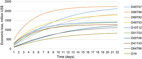
Demand-side inoperability and the resulting economic losses are the two metrics that were obtained from the inoperability input–output model. While the former describes the percentage difference between the ordinary business activity of a sector and its current level of production, the latter quantifies the total damage in monetary values, accounting for ripple effects. Both ratios have to be considered when carrying out a sector risk assessment as they may yield to different sector rankings. This is attributable, among other reasons, to the different production volumes of the sectors (Santos 2006). It is therefore advantageous for the interpretation if the damage is put into the relative ratio of the total production of the sector. This fact should also be addressed when defining and designing precautionary measures against cyber risks (i.e., whether the actions minimize the inoperability or the economic loss). Moreover, the individual inoperability level allows evaluating the preparedness of the respective economic sector to recover from disruptive cyberattacks (Ali and Santos 2014).

The 10 sectors with the highest cumulative economic losses (in US$million) and their respective average inoperability values of scenario 1 are summarized in Table 4. The total cumulative economic loss amounted to US$23.2 billion.

TABLE 4 Top 10 Affected Sectors Based on Average Inoperability

		Economic loss		Average inoperability
Sector	Name	Rank	Value (mUS$)	Rank	Value (%)^26
D45T47	Wholesale and retail trade; repair of motor vehicles	1	2,283	19	0.36%
D86T88	Human health and social work	2	2,255	14	0.46%
D69T82	Human health and social work	3	1,997	20	0.32%
D49T53	Transportation and storage	4	1,846	3	0.83%
D10T12	Food products, beverages and tobacco	5	1,440	8	0.64%
D01T03	Agriculture, forestry, and fishing	6	1,424	1	1.29%
D05T06	Mining and extraction of energy producing products	7	1,344	2	0.98%
D41T43	Construction	8	1,306	13	0.51%
D64T66	Financial and insurance activities	9	1,202	25	0.19%
D19	Coke and refined petroleum products	10	0,878	16	0.42%

Figures 1 and 2 show the development of the inoperability and the cumulative economic loss of the top 10 affected sectors, respectively.

FIGURE 1. Inoperability Development of the Top 10 Inoperable Sectors.

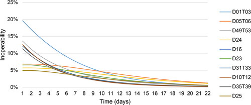
FIGURE 2. Cumulative Economic Losses for the Top 10 Affected Sectors.

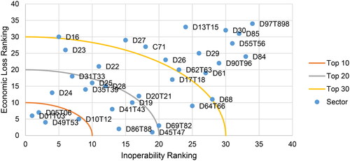
The sectors with the highest inoperability may not be those with the highest economic losses, and vice versa. To visualize this, Resurreccion and Santos (2012) present dynamic cross-prioritization plots, where each point represents the relative position of a sector in terms of its ordinal ranks with respect to inoperability and economic loss (see Figure 3). The use of a quarter ellipse represents a threshold for capturing critical sectors. It is possible to vary the preferences (i.e., whether a higher threshold should be assigned to one or the other criteria). In the following graphs, the three quarter circles indicate the top 10, top 20, and top 30 zones, respectively. In order for a sector to be classified in the respective category, both the inoperability rank and the economic loss rank must be below the threshold (i.e., the top 10 zone does not necessarily contain 10 sectors). The figures depicting the inoperability curves, cumulated economic losses and dynamic cross-prioritization plots for the other scenarios are presented in Appendix E. Appendix F illustrates all necessary steps of the calculations in detail and also provides a link to an excel tool.

FIGURE 3. Dynamic Cross-Prioritization Plot.

5.2. Aggregate Results Across all Scenarios

Table 5 presents the total economic losses of the six scenarios. It must be borne in mind that these scenarios differ in terms of affected sectors, inoperability, and recovery time. In the industry studies cited, the scenarios differ in terms of the affected countries. To improve comparability we simulate all scenarios for the United States. Other countries can, however, easily be added with the input–output transaction tables provided by the OECD (2018).

TABLE 5 Summary of Total Economic Losses by Scenario

Scenario	Risk factor	Total economic damage (mUS$)
		Mean	Variation inoperability only					Variation inoperability & recovery time
			Min	Max	Range	Range/mean	Min		Max	Range	Range/mean
1)	Supervisory control and data acquisition network/industrial control system extortion	23,220	11,610	34,830	23,220	1.00	11,610		34,830	23,220	1.00
2)	Cloud service failure	722	—	—	—	—	542		1,264	722	1.00
3)	Health sector and hospitals	28,481	5,178	51,784	46,606	1.64	6,214		62,141	55,927	1.96
4)	Municipal services	23,261	—	—	—	—	—		—	—	—
5)	Telecommunication	1,521	—	—	—	—	—		—	—	—
6)	Cross-sector attack	34,881	26,756	43,186	16,430	0.47	24,160		47,112	22,952	0.66

Regarding the means presented in column three of Table 5, the loss estimations for five of the six scenarios are in a range from US$0.7 to 28.5 billion. The most extreme scenario is the cross-sector attack scenario with a damage estimation of US$34.9 billion. This value would be among the top 10 in terms of largest loss events, but it is significantly smaller than the biggest catastrophic losses documented in history, which are the Japan earthquake and tsunami in 2011 with an estimated economic loss of US$210 billion and Hurricane Katrina in 2005 with an estimated economic loss of US$125 billion (see Munich Re 2016). Overall, it thus seems that the scenarios are inside the range of insurability and in principal can be covered by the traditional insurance and reinsurance market (or at least comparable numbers have been covered by the traditional insurance and reinsurance market; for example, the insured loss for Hurricane Katrina was US$40 billion; see Munich Re 2016).

Regarding the variation of the loss estimators, we present minimum and maximum values by (a) varying the inoperability values only or (b) by varying both inoperability and recovery time. For scenario 2 the inoperability value is predefined as one fixed number, while for scenarios 4 and 5 both inoperability and recovery time were fixed. For all others, inoperability and recovery time were given in a corridor.²⁵ Applying these corridors, the most extreme variation can be observed for the health sector scenario with loss estimators from US$5 to 62 billion. The minimum and maximum values are at least 23% lower/24% higher (scenario 7: variation of inoperability only) and vary up to values that are 78% lower/118% higher (scenario 3: variation inoperability and recovery time). All these variations illustrate the large uncertainty underlying the loss estimations, but are useful to provide some indication for the potential economic magnitude of the scenarios.

The results presented here provide an indication of the potential loss severity given a cyber event, but they do not provide estimations for the likelihood of the same. Of course, it is difficult to estimate the probability of these loss events. But at least it is possible to say that some of the scenarios have already happened in the past (such as scenario 5, for example), while other events such as a cross-sector attack are more hypothetical. This might be an indication that an extreme loss scenario like a cross-sector attack is similarly unlikely to other loss events.

6. CONCLUSIONS

This article assesses the impact of six widely discussed cyberattack scenarios in terms of inoperability and economic damage. We apply the dynamic input–output model tool to consistently estimate the economic losses of various cyber risk scenarios, including ripple effects. The utilization of fuzzy values allows determining the sensitivity of the inoperability rankings to different input parameters. The combination of the qualitative categorization of cyber risk scenarios using a standardized taxonomy with the quantitative estimation of economic losses enables a holistic view and allows comparability and scalability for future studies. The economic losses of six well-known cyber risk scenarios range from $0.7 to $35 billion; the potential economic losses fall within the realm of insurability in all our scenarios. Importantly, the specific dollar values are not the main finding of the article. Rather, the qualitative context plays a sizeable role in the economic impact analysis, which is generally not captured in models that attempt to assess economic impact (in the cyber world at least). Policymakers and other decision makers can use our results to qualitatively ascertain how new scenarios they are confronted with fit into our scenario framework and thus arrive at a rough order of magnitude estimate of its economic impact; they also might assess the need for government backstops and other market-intervening tools. Additionally, organizations might determine the optimal amount to spend on information security using this method. As organizations identify which extreme scenarios are most relevant to their operating context, they can more appropriately plan and budget for the relevant extreme scenario accordingly. For example, this may include allocating additional funds to cyber insurance premiums to improve coverage.

Actuaries and other insurance professionals are increasingly facing cyber risks, both in the underwriting as well as in the operational risks of the insurance companies. For this reason, we see at least two aspects both groups of professionals can gain from this article: First, the article provides standardized information and comparisons on a set of the most relevant cyber risk scenarios that so far do not exist (due to the lack of comparability in the industry studies where they are presented); this might provide useful input in discussions on developing cyber insurance products and in the risk management of insurance companies. Second, our article provides at least indicative information on the economic magnitude of these events, information that also did not exist in a standardized and consistent form so far. Although we certainly do not claim that our dollar values are point estimates, insurance managers and other professionals can use our results to evaluate the relevance (i.e., potential duration and severity) of different scenarios.

We also emphasize that the results are of interest not only for the actuarial and insurance business domain, but also for a broader risk management and insurance economist audience. Risk managers in companies outside the insurance field need to get a better understanding of the economic magnitude of different cyber risk scenarios, and to be able to build proper risk management strategies. Insurance economists need to analyze the potential welfare implications of selected cyber scenarios, for example, to assess impact on critical infrastructure or to evaluate the need for government interventions in case of adverse events. All this is not possible at this stage, because of the limited comparability of the scenarios discussed in industry studies.

Our article opens several avenues for future research in the area of business, economics, and actuarial science. For example, one limitation of the article is that it depends on various assumptions, many of which are derived based on subjective expert opinions. Nevertheless, given the transparent and standardized approach the article uses, it provides a first step toward a more objective and comparable analysis of the scenarios that are widely discussed among academics and practitioners. But also, these scenarios are based on some historical considerations—that is, they describe events that happened in the past or events that were realistic in the past. Given the dynamic nature of cyber risk, one might argue that these historical considerations are not necessarily a good indication of future events. There are other elements not modeled in the article, such as potential correlation across scenarios or multiple events in a year, which might further inflate the potential loss estimates. With these limitations in mind, the scenarios and their order-of-magnitude quantitative loss estimates are still informative for both policy and organizational analysis and insight. The increasing use of digital technologies in the postpandemic world has further increased the importance of the analyses we present in the article, but again also emphasizes the dynamic nature of cyber risk events.

Even though various features of the fuzzy dynamic input–output methodology were displayed, other factors and methods need to be considered. For example, the input–output model does not include reputational damage and physical losses that could result from cyberattacks. The input–output model is based on pure demand reductions. However, cyberattacks do not lead only to demand reductions; for example, a cyberattack may lead to additional demand for computer software. Moreover, this method does not address how well risk management (e.g., cyber insurance) is structured with regard to specific cyberattacks; we also do not include any regulatory considerations (see, e.g., Kashyap and Wetherilt 2019). Finally, the input–output model and the input–output tables provided by the OECD allowed only a static analysis. Also, potential responses, for example, by the government, might vary depending on the scenario and are not modeled in the article. Further, it has to be borne in mind that the traditional input–output model provides an upper bound estimate of economic losses (Rose and Liao 2005). In the future, a close look at emerging trends and potential cyberattack scenarios is necessary. Ways to incorporate economic losses resulting from other than demand-side perturbations (e.g., reputational damage) must be developed. Insights from the operational risk literature (e.g., Eckert and Gatzert 2017) might be used to incorporate reputational effects also in the cyber risk analysis (see, e.g. Egan et al. 2019). In general, our analysis provides a rather narrow perspective on the economic impact of extreme cyber risk scenarios, also because a broader perspective is not really achievable in the space constraints imposed by journals. For a broader perspective we refer to Coburn et al. (2019).

Given the manifold assumptions and the risk of change, the sensitivity analysis presented in the article is important. The variation of the loss estimates is large in many cases, emphasizing the high uncertainty in the loss estimators. The mean loss estimators presented in the article should thus not be interpreted as point estimates under certainty, but rather as distributions that are uncertain. This situation might be compared with the beginning of the economic impact modeling for natural disasters, when data were also scarce and estimates were correspondingly difficult. Given the increase in recorded losses from cyberattacks in recent years and the expected increase in frequency and severity of cyber risks as a result of globalization and digitization, it is imperative for policymakers to have reliable information about the potential impact of cyber risks. Our study offers an approach to identify the potential economic magnitude of cyber risk for vulnerable critical infrastructure sectors, while capturing the qualitative context of the scenarios in the economic projection.

Discussions on this article can be submitted until April 1, 2024. The authors reserve the right to reply to any discussion. Please see the Instructions for Authors found online at http://www.tandfonline.com/uaaj for submission instructions.

Notes

1 The actuarial literature so far mainly focuses on modeling of cyber risk (e.g., Fahrenwaldt et al. 2018; Xu and Hua 2019; Sun et al. 2020; Jevtić and Lanchier 2020; Farkas et al. 2020) and empirical analysis of the cyber insurance market (e.g., Cole and Fier 2020; Kamiya et al. 2021). The methodological foundation of our article is the dynamic input output inoperability model, which is based on the Leontief (1974) input–output model and has been developed and used in other contexts (Haimes and Jiang 2001). The two papers closest to our analyses are one by the RAND Corporation (Dreyer et al. 2018), which develops a methodology for estimating the global costs of cyber risk, and a paper by Bounfour et al. (2018), who use the dynamic input–output inoperability model to analyze the impact of cyberattacks on the telecommunications and finance sector. The idea of our analysis is to expand these two papers by examining the impact of six widely discussed cyber risk scenarios and filter out values for inoperability and recovery time based on this literature (i.e., historical data and expert opinions, rather than assumptions that are not further justified or motivated).

2 The insured losses for the Japanese tsunami in 2011 were US$40 billion, and for Hurricane Katrina in 2005 they were US$60 billion, illustrating the capacity and realm of insurability (see Munich Re 2016).

3 See Eling and Schnell (2016). The focus of this article is on cyberattacks, but we acknowledge that certain cyber risks are also not attacks, such as, for example, the unintended disclosure of information.

4 An infrastructure is termed critical if its disruption or destruction has a significant impact on health, safety, security, or economic or social well-being of people (Council Directive 2008/114/EC).

5 See, e.g., Börjeson et al. (2006) and van Notten et al. (2003) for a general description of the typology and classification of scenarios.

6 Direct costs include the costs borne directly by the sector(s) targeted by the cyberattack (e.g., business interruptions, litigation costs, and fines), while systemic costs comprise the macroeconomic impact on productivity experienced by the nonaffected sectors due to the direct damage in the sector(s) affected by the cyberattack (Dreyer et al. 2018).

7 They found that cybercrime results in total costs of US$799 billion to 22.5 trillion (1.1 to 32.4 percent of global GDP). In additional material available upon request we also include a solar storm, but we excluded it from the analysis presented in the main body of this article because it is caused by a natural geophysical phenomenon.

8 See Jin et al. (2018) for an application of an econometric model to evaluate the loss due to surge disasters in China.

9 See Feenstra and Sasahara (2018) for a quantification of the impact on U.S. employment from imports and exports between 1995 and 2011, applying input–output analysis.

10 See Kajitani and Tatano (2018) for a recent discussion about the applicability of the computable general equilibrium model to assess short-term economic impacts of natural disasters. Computable general equilibrium models are also referred to as applied general equilibrium models (Ballard and Johnson 2017).

11 See Leontief (1951; 1966; 1974). A comprehensive introduction to the model and its applications is provided by Miller and Blair (2009).

12 Inoperability is defined as the deviation of the actual activity level from the planned operation level (Niknejad and Petrovic 2016).

13 Jung et al. (2009).

14 The baseline final production refers to the volume of production in the absence of economic disturbance. Degraded is the reduced production volume with economic disturbance.

15 Lian and Haimes (2006) extended the original dynamic inoperability input–output model to a continuous version.

16 It is generally assumed that a sector has recovered from an external disruption if the activity level reaches 99% of the preshock activity level. This is justified by the fact that the restoration of the last percentage requires a considerable amount of time, whereas the economic performance is almost intact again.

17 Supervisory control and data acquisition networks are one of the most common types of industrial control systems. They monitor and control assets distributed over large geographical areas and use specific control equipment (Cherdantseva et al. 2016).

18 See Dejung (2017).

19 See Dejung (2017), Risk Management Solutions, Inc. (2016), and World Economic Forum (2014).

20 See Dejung (2017).

21 See Trautman and Ormerod (2018).

22 See Dejung (2017).

23 See Risk Management Solutions, Inc. (2016) and Ruffle et al. (2014).

24 Due to the methodology chosen, the economic losses of some scenarios cannot be estimated. This applies, for example, to data breaches, as these do not affect the operability of the economy. See, for example, the cyber data exfiltration scenario proposed by Risk Management Solutions, Inc. (2016).

25 We also present the range over the mean as relative variation measure, following the idea of the coefficient of variation, where the standard deviation is divided by the mean. Note that the reason why we do not vary the inoperability value for scenario 2 and both inoperability and recovery time for scenarios 4 and 5 was that these values were fixed in the studies we cite to develop Table 3, while all other parameters for all other scenarios were given as corridors. It is possible to also vary the values fixed in Table 3 (and Table 5 consequently), but this requires another subjective set of assumptions.

26 The average inoperability value is defined as the business interruption recorded in the respective sector for the assumed recovery time. The time frame for the calculation of the average inoperability values therefore varies from one scenario to another.

REFERENCES

- Ali, J., and J. R. Santos. 2014. Modeling the ripple effects of IT-based incidents on interdependent economic systems. Systems Engineering 18(2): 146–61. doi:10.1002/sys.21293
- Bounfour, A., R. Dieye, N. Kammoun, and A. Ozaygen. 2018. Macro estimates of intangibles cyber-risks. https://www.hermeneut.eu/wp-content/uploads/2018/08/HERMENEUT-D3.2-Macro-estimates-of-intangibles-cyber-risks.pdf (accessed April 20, 2021).
- Cherdantseva, Y., P. Burnap, A. Blyth, P. Eden, K. Jones, H. Soulsby, and K. Stoddart. 2016. A review of cyber security risk assessment methods for SCADA systems. Computers & Security 56: 1–27. doi:10.1016/j.cose.2015.09.009
- Chigada, J., and R. Madzinga. 2021. Cyberattacks and threats during COVID-19: A systematic literature review. South African Journal of Information Management 23(1): 1–11.
- Cimellaro, G. P., A. M. Reinhorn, and M. Bruneau. 2010. Framework for analytical quantification of disaster resilience. Engineering Structures 32(11): 3639–49. doi:10.1016/j.engstruct.2010.08.008
- Coburn, A., E. Leverett, and G. Woo. 2019. Solving cyber risk. Hoboken, NJ: Wiley.
- Cole, C. R., and S. G. Fier. 2020. An empirical analysis of insurer participation in the U.S. cyber insurance market. North American Actuarial Journal. doi:10.1080/10920277.2020.1733615
- Dejung, S. 2017. Economic impact of cyber accumulation scenarios. Swiss Insurance Association Cyber Working Group.
- Dreyer, P., T. Jones, K. Klima, J. Oberholtzer, A. Strong, J. Welburn, and Z. Winkelman. 2018. Estimating the global cost of cyber risk: methodology and examples. doi:10.7249/rr2299https://www.rand.org/pubs/research_reports/RR2299.html (accessed April 20, 2021).
- Eckert, C., and N. Gatzert. 2017. Modeling operational risk incorporating reputation risk: An integrated analysis for financial firms. Insurance: Mathematics and Economics 72: 122–37. doi:10.1016/j.insmatheco.2016.11.005
- Egan, R., S. Cartagena, R. Mohamed, V. Gosrani, J. Grewal, M. Acharyya, et al. 2019. Cyber operational risk scenarios for insurance companies. British Actuarial Journal 24(6): 1–34. doi:10.1017/S1357321718000284
- Eling, M., and W. Schnell. 2020. Capital requirements for cyber risk and cyber risk insurance. North American Actuarial Journal 24(3): 370–92. doi:10.1080/10920277.2019.1641416
- Fahrenwaldt, M. A., S. Weber, and K. Weske. 2018. Pricing of cyber insurance contracts in a network model. ASTIN Bulletin 48(3): 1175–218. doi:10.1017/asb.2018.23
- Falco, G., M. Eling, D. Jablanski, M. Weber, V. Miller, L. A. Gordon, S. S. Wang, J. Schmit, R. Thomas, M. Elvedi, T. Maillart, E. Donavan, S. Dejung, E. Durand, F. Nutter, U. Scheffer, G. Arazi, G. Ohana, and H. Lin. 2019. Cyber risk research impeded by disciplinary barriers. Science 366(6469): 1066–69. doi:10.1126/science.aaz4795
- Falco, G., A. Viswanathan, C. Caldera, and H. Shrobe. 2018. A master attack methodology for an AI-based automated attack planner for smart cities. IEEE Access 6: 48360–73. doi:10.1109/ACCESS.2018.2867556
- Farkas, S., O. Lopez, and M. Thomas. 2021. Cyber claim analysis using Generalized Pareto regression trees with applications to insurance. Insurance: Mathematics and Economics 98: 92–105. doi:10.1016/j.insmatheco.2021.02.009
- Haimes, Y. Y., and P. Jiang. 2001. Leontief-based model of risk in complex interconnected infrastructures. Journal of Infrastructure Systems 7(1): 1–12. doi:10.1061/(ASCE)1076-0342(2001)7:1(1)
- Haimes, Y. Y., B. M. Horowitz, J. H. Lambert, J. R. Santos, C. Lian, and K. G. Crowther. 2005. Inoperability input-output model for interdependent infrastructure sectors. Journal of Infrastructure Systems 11(2): 67–79. doi:10.1061/(ASCE)1076-0342(2005)11:2(67)
- Holling, C. S. 1973. Resilience and stability of ecological systems. Annual Review of Ecology and Systematics 4(1): 1–23. doi:10.1146/annurev.es.04.110173.000245
- Howard, J. D. 1997. An analysis of security incidents on the Internet. PhD thesis, Carnegie Mellon University. https://resources.sei.cmu.edu/library/asset-view.cfm?assetid=52454 (accessed April 20, 2021).
- Howard, J. D. 2015. Using a common language for computer security incident information. In Computer Security Handbook, ed. S. Bosworth, M. E. Kabay, and E. Whyne, 8.1–8.21. Hoboken, NJ: John Wiley & Sons. doi:10.1002/9781118851678.ch8
- Jevtić, P., and N. Lanchier. 2020. Dynamic structural percolation model of loss distribution for cyber risk of small and medium-sized enterprises for tree-based LAN topology. Insurance: Mathematics and Economics, 91: 209–23. doi:10.1016/j.insmatheco.2020.02.005
- Jung, J., J. R. Santos, and Y. Y. Haimes. 2009. International trade inoperability input-output model (IT-IIM): theory and application. Risk Analysis 29(1): 137–54. doi:10.1111/j.1539-6924.2008.01126.x
- Kamiya, S., J. K. Kang, J. Kim, A. Milidonis, and R. M. Stulz. 2021. Risk management, firm reputation, and the impact of successful cyberattacks on target firms. Journal of Financial Economics 139(3): 719–49. doi:10.1016/j.jfineco.2019.05.019
- Kashyap, A. K., and A. Wetherilt. 2019. Some principles for regulating cyber risk. AEA Papers and Proceedings 109: 482–87. doi:10.1257/pandp.20191058
- Kelly, S., E. Leverett, E. J. Oughton, J. Copic, S. Thacker, R. Pant, L. Pryor, G. Kassara, T. Evan, S. J. Ruffle, M. Tuveson, A. W. Coburn, D. Ralph, and J. W. Halls. 2016. Integrated infrastructure: Cyber resiliency in society: Mapping the consequences of an interconnected digital economy. https://www.jbs.cam.ac.uk/fileadmin/user_upload/research/centres/risk/downloads/crs-integrated-infrastructure-cyber-resiliency-in-society.pdf (accessed April 20, 2021).
- Lagazio, M., N. Sherif, and M. Cushman. 2014. A multi-level approach to understanding the impact of cyber crime on the financial sector. Computers & Security 45: 58–74. doi:10.1016/j.cose.2014.05.006
- Lallie, H. S., L. A. Shepherd, J. R. Nurse, A. Erola, G. Epiphaniou, C. Maple, and X. Bellekens. 2021. Cyber security in the age of Covid-19: A timeline and analysis of cyber-crime and cyber-attacks during the pandemic. Computers & Security 105: 102248. doi:10.1016/j.cose.2021.102248
- Leontief, W. W. 1951. The structure of the American economy, 1919–1939: An empirical application of equilibrium analysis. New York, NY: Oxford University Press.
- Leontief, W. W. 1966. Input-output economics. Oxford: Oxford University Press.
- Leontief, W. W. 1974. Structure of the world economy: Outline of a simple input-output formulation. American Economic Review 64(6): 823–34.
- Lewis, J. A. 2018. Economic impact of cybercrime—No slowing down. Santa Clara, CA: McAfee. https://csis-website-prod.s3.amazonaws.com/s3fs-public/publication/economic-impact-cybercrime.pdf (accessed April 20, 2021).
- Li, Y., and Q. Liu. 2021. A comprehensive review study of cyber-attacks and cyber security; Emerging trends and recent developments. Energy Reports 7: 8176–86. doi:10.1016/j.egyr.2021.08.126
- Lian, C., and Y. Y. Haimes. 2006. Managing the risk of terrorism to interdependent infrastructure systems through the dynamic inoperability input-output model. Systems Engineering 9(3): 241–58. doi:10.1002/sys.20051
- Lian, C., J. R. Santos, and Y. Y. Haimes. 2007. Extreme risk analysis of interdependent economic and infrastructure sectors. Risk Analysis 27(4): 1053–64. doi:10.1111/j.1539-6924.2007.00943.x
- Miller, R. E., and P. D. Blair. 2009. Input-output analysis: Foundations and extensions. Cambridge University Press.
- Munich Re. 2016. Loss events worldwide 1980–2015. https://reliefweb.int/sites/reliefweb.int/files/resources/Loss_events_worldwide_1980-2015.pdf (accessed April 20, 2021).
- Niknejad, A., and D. Petrovic. 2016. A fuzzy dynamic inoperability input-output model for strategic risk management in global production networks. International Journal of Production Economics 179: 44–58. doi:10.1016/j.ijpe.2016.05.017
- Nikolakopoulos, T., E. Darra, and D. Tofan. 2016. The cost of incidents affecting CIIs: Systematic review of studies concerning the economic impact of cyber-security incidents on critical information infrastructures (CII). Heraklion: ENISA.
- Organization for Ecoomic Cooperation and Development. 2018. Input-output tables 2018 edition. https://stats.oecd.org/Index.aspx?DataSetCode=IOTSI4_2018 (accessed April 20, 2021).
- Panzieri, S., and R. Setola. 2008. Failures propagation in critical interdependent infrastructures. International Journal of Modelling, Identification and Control 3(1): 69–78. doi:10.1504/IJMIC.2008.018186
- Parenty, T. J., and J. J. Domet. 2019. Sizing up your cyberrisks. Harvard Business Review 97(6): 102–10.
- Resurreccion, J., and J. R. Santos. 2012. Multiobjective prioritization methodology and decision support system for evaluating inventory enhancement strategies for disrupted interdependent sectors. Risk Analysis 32(10): 1673–92. doi:10.1111/j.1539-6924.2011.01779.x
- Risk Management Solutions, Inc. 2016. Managing cyber insurance accumulation risk. https://www.jbs.cam.ac.uk/fileadmin/user_upload/research/centres/risk/downloads/crs-rms-managing-cyber-insurance-accumulation-risk.pdf (accessed April 20, 2021).
- Rose, A., and S.-Y. Liao. 2005. Modeling regional economic resilience to disasters: A computable general equilibrium analysis of water service disruptions. Journal of Regional Science 45(1): 75–112. doi:10.1111/j.0022-4146.2005.00365.x
- Ruffle, S. J., G. Bowman, F. Caccioli, A. W. Coburn, S. Kelly, B. Leslie, and D. Ralph. 2014. Stress test scenario: Sybil logic bomb cyber catastrophe. Cambridge Risk Framework Series. Centre for Risk Studies, University of Cambridge.
- Santos, J. R. 2006. Inoperability input-output modeling of disruptions to interdependent economic systems. Systems Engineering 9(1): 20–34. doi:10.1002/sys.20040
- Smith, Z. M., E. Lostri, and J. A. Lewis. 2021. The hidden costs of cybercrime. https://www.csis.org/analysis/hidden-costs-cybercrime.
- Sun, H., M. Xu, and P. Zhao. 2020. Modeling malicious hacking data breach risks. North American Actuarial Journal. doi:10.1080/10920277.2020.1752255
- Trautman, L. J., and P. Ormerod. 2018. Wannacry, ransomware, and the emerging threat to corporations. Tennessee Law Review 86: 503–56.
- Weintraub, R., and J. Borenstein. 2017. 11 Things the health care sector must do to improve cybersecurity. Harvard Business Review Online. https://hbr.org/2017/06/11-things-the-health-care-sector-must-do-to-improve-cybersecurity (accessed April 20, 2021)
- World Bank. 2019. GDP (current US$). https://data.worldbank.org/indicator/ny.gdp.mktp.cd (accessed April 20, 2021).
- World Economic Forum. 2014. Global risks 2014 ninth edition. http://reports.weforum.org/global-risks-2014/?doing_wp_cron=1548774994.0724980831146240234375 (accessed April 20, 2021).
- Xu, M., and L. Hua. 2019. Cybersecurity insurance: Modeling and pricing. North American Actuarial Journal 23(2): 220–49. doi:10.1080/10920277.2019.1566076