
Abstract
This study was aimed to evaluate the freshness and quality of cultured shrimp (litopenaeus vannamei) during 9 days of storage on ice (i.e., at a temperature of 0°C) using image processing technique. A lighting chamber was used to provide uniform conditions for illumination. The shrimp freshness was evaluated using computer vision technique through color changes of head, legs and tail of the harvested shrimps. Thirty-six color parameters of the images such as mean and variance of red (r), green (g), blue (b), lightness hue (h), saturation (s), value (v), luma information (i and y), the luma component (y), chroma component (cr), lightness (L*), redness (a*), yellowness (b*), chroma (c), and hue (h) were analyzed. Some parameters, such as b*, from side pictures and r mean, b variance, v mean, y mean, b* mean and (L*) mean from top pictures changed with a rather similar trend during the storage period. Different computational expert approaches such as linear discriminant analysis, quadratic discriminant analysis, K nearest neighbors, and discriminant partial least squares regression were examined for shrimp freshness classification. For this, all the variables and the subsets of variables were selected by means of stepwise linear discriminant analysis, stepwise orthogonalization, classification and regression trees. The shrimp freshness was characterized with a high classification accuracy of 90%. Freshness evaluation using image processing is proposed as a potential technique to the food industry.
INTRODUCTION
Shrimp is one of the most delicious seafood, with a high nutritional value and many health benefits.[Citation1] From different types of shrimp, pacific white shrimp (litopenaeus vannamei) makes up about 90% of the shrimp aquaculture in the western hemisphere and its global harvest is on the increase.[Citation2] Increasing production and consumption of shrimp can cause to double the importance of its freshness and quality in shrimp industry. Determination of the quality indicators is one of the interesting topics in food engineering and the respective industry. For instance, freshness as a qualitative index, is one of the main parameters for evaluating the food products and their preferences by consumers.[Citation3–Citation5]
Shrimp color change depends on several factors of which the microbiological and chemical processes such as changes in protein, lipid fractions, and system of natural enzymes are of particular importance. Existing enzymes in the air may also cause chemical changes on the surface of the shrimp leading to the formation of brown spots near the shrimp surfaces and shell.[Citation3]
Color change of shrimp usually emerges with spots or melanoses being nutritionally harmless but with unpleasant color appearing mainly along the head, swimmerets, tail, and close to shell areas.[Citation6] Some studies have shown that the quality and freshness of sea foods during storage are strongly related to their color.[Citation2,Citation7] Similarly, color can be an important feature in freshness evaluation of shrimp. Freshness and food quality grading system by image processing is based on visual characteristics such as color, texture, and morphology as pointed out by Nagalakshmi et al.[Citation8] This system offers a low-cost, fast-response, and highly accurate technique for food quality grading.
The shrimp freshness and quality can be determined using a range of destructive and non-destructive methods including the sensory methods (e.g., quality index method [qim], torry scheme, etc.), physical methods (e.g., texture analysis, torrymeter, electronic nose, and near-infrared reflectance spectroscopy), chemical and biochemical methods (e.g., total volatile basic nitrogen, trimethylamine, pH, atp, etc.), and microbiological methods (i.e., the total plate count of bacterial load).[Citation9,Citation10] Sun et al.[Citation11] studied the effect of grape seed extracts (GSE) on the melanosis and quality of pacific white shrimp during storage on ice. Their results suggested that GSE could be used as an efficient natural agent to hinder postmortem melanosis to improve the quality of shrimp during storage.
The quality or freshness evaluation of the aquatic foods has been previously reported.[Citation12,Citation13] However, only a few studies can be found that apply computer vision systems for quality evaluation of shrimp. For instance, Luzuriaga et al.,[Citation14] developed an automated device in red-green-blue (RGB) color space for diagnosing melanosis and detection of foreign objects. Their machine vision system measured the percent area of melanosis on white shrimp (penaeus setiferus) stored on ice for up to 17 days. Melanosis was measured and predicted with grading of a trained sensory panel. This approach could objectively characterize the visual quality indices of white shrimp. The aim of this study was to assess the potential of image analysis (color and texture properties) as a reliable method for shrimp freshness evaluation. For this purpose, several computational expert approaches were used.
MATERIALS AND METHODS
Pacific white shrimps, weighing between 10 to 25 g, were purchased from a shrimp farm in Booshehr, Iran. Immediately after harvesting, the shrimps were dipped into sodium sulfites, then transported to the laboratory in polystyrene boxes filled with ice. All shrimps were stored on ice at a temperature of 0–4°C for 9 days. For avoiding the contact between shrimps and the accumulated water, every 10 shrimps were packed into a plastic pocket. Imaging was performed immediately after harvest and every 72 h, i.e., on the 3rd, 6th, and 9th days of storage.
The image processing system consisted of a dark chamber and lighting system, a digital camera, computer hardware, and software. For a proper illumination of the shrimp samples, some light-emitting diode (LED) lamps with white and yellow colors were installed on the upper part of the dark chamber. To prevent the direct incidence of light to the sample and its reflection, polyvinyl chloride (PVC) sheets were used in front of the lamps. The lighting box was made with aluminum. To minimize the background light and light reflectance, the interior walls of the lighting chamber were covered with black sheet. To adjust the distance between the samples and camera, the chamber was equipped with a knob adjusted by rotary moving. The best quality of image was found at a distance of 11 cm over the sample. A charge-coupled device (CCD) power shot color camera (Sony dsc-w530 digital color camera, Japan,) with remote capturing capability was employed to take images from the shrimp samples. The camera was connected to a laptop (ASUS, k43sa, China) through universal serial bus (USB) port. The shrimp sample was located on the center of the background (). Images were captured with a five megapixel resolution. For stable lighting, the camera and LED lamps were turned on 10 min before capturing the images. For calibrating the camera, the white balance adjustment was manually applied. All images were taken with the same camera specifications (exposure mode: manual, no zoom, no flash, image type: jpeg). After setting the best illumination, skin images of 80 shrimps on four days (0, 3, 6, and 9 days of storage) were taken by means of the digital camera and the resulting images were transferred to the computer. The required programs for processing the images and extracting the desired features were written using the image processing functions in MATLAB software.[Citation15] Freshness of the shrimp was then characterized based on the four categories of freshness (i.e., four storage days). Characterization was based on texture and color parameters of skin including average color of the head, legs, and the tail.
FIGURE 1 A: Lighting chamber for image capturing; B: shrimp side pictures; and C: shrimp top pictures.
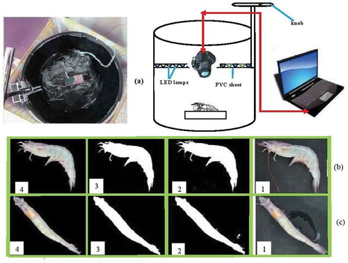
The image preprocessing steps are presented in and . Image pre-processing generally includes suppressing the low-frequency background noise, normalizing the intensity of each image particle to correct the geometric distortions, grey level, blurring, and omitting the reflections and image portion masking. After image acquisition and storage, all images were in a “jpeg” format with a resolution of 757 × 1050 with RGB color mode. A black background was used for each sample for imaging ( and ). All images were converted to binary image and Otsu thresholding method was used for separating the particles from the background.[Citation16,Citation17] Then, the resulting image was subtracted from the original image (Figs. 1b2 and 1c2). Moreover, voids in the resulting image were filled with their neighboring intensities (Figs. 1b3 and 1c3). The features were then extracted from the basic color image combined with the binary image (Figs. 1b4 and 1c4). The data matrix has 80 rows (objects, i.e., 20 shrimp samples for each storage time) and 66 columns (i.e., variables). The variables are defined in .
TABLE 1 The variables extracted from the images captured
TABLE 2 Statistics of the variables
TABLE 3a General fisher weights
TABLE 3b Fisher weights for categories 1 and 2
TABLE 3c Fisher weights for categories 1 and 3
TABLE 3d Fisher weights for categories 1 and 4
TABLE 3e Fisher weights for categories 2 and 3
TABLE 3f Fisher weights for categories 2 and 4
TABLE 3g Fisher weights for categories 3 and 4
Data analysis was performed in MATLAB by means of explorative analysis (principal components analysis) and the following classification techniques:[Citation18] (1) linear discriminant analysis (LDA), (2) quadratic discriminant analysis (QDA), (3) K nearest neighbors (KNN), and (4) discriminant partial least squares regression (D-PLS). The items, both from the variables and the subsets of variables, were selected by means of stepwise-LDA (STEP-LDA), Stepwise orthogonalization (SELECT), and classification and regression trees (CART).[Citation5]
RESULT AND DISCUSSION
shows the changes in color of different parts of shrimp body during storage on ice for 9 days. It is clear that the color of shrimp head, tail, and legs changed sequentially to orange color (3rd day), brown (6th day), and dark (9th day) during the period of storage. This could be attributed to the activity of microorganisms leading to organoleptic changes in color and appearance of shrimp after death.[Citation19] Okpala et al.[Citation20] found that color changes of pacific white shrimp freshly harvested is associated with the development of rancid odors during frozen storage. Also, the metric chroma (c) and total color difference (TCD) could be used to determine freshness and shelf life of pacific white shrimp freshly harvested and stored on ice. Their results were not in agreement with the color data of deep water pink shrimp (parapenaeus longirostris) processed on board with ice as found by Huidobro et al.[Citation21]
FIGURE 2 Cultured shrimp color changes during storage on ice.
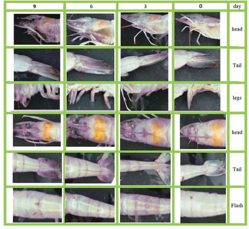
As illustrated in , on the day 0 (i.e., immediately after harvest) no melanosis, flesh, and spot could be found on shrimp skin. On the third day, a small part of the shrimp head, legs, and tail became slightly dark. Black dots may not be harmful but can be an indication of poor cooling, transportation, and storage of shrimp after harvest. shows that the means of r, g, and b of side pictures decreased during shrimp storage. This observation could be related to increase in melanosis during storage time. The h and s increased until the 6th day and slightly decreased between 6th to 9th days while v continuously decreased over the 9 days as shown in . The change trends of L*, a*, and b* during storage are depicted in . It can be seen that L* decreased over the storage time while a* and b* did not show any significant change.
FIGURE 3 The color change of four groups of pacific white shrimps (litopenaeus vannamei) during 9 days of storage on ice.
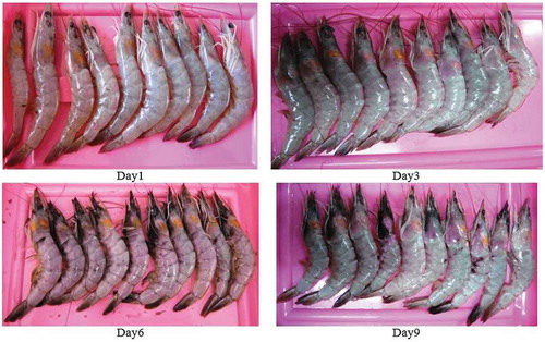
FIGURE 4 Variation of shrimp color parameters from side pictures during storage on ice; A: r, g, and b; B: h, s, and v; C: L*, a*, and b*; and D: c and h.Day: 1 = first day, 2 = third day, 3 = sixth day, 4 = ninth day; h = hue, c = chroma.
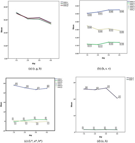
shows the change in chroma (c) and hue (h). The hue rapidly increased until the 6th day followed by a sharp decrease between the 6th to 9th day. However, the chroma remained almost constant. Similar variations were found for the color parameters of top pictures (not shown). A completely randomized block design was used for statistical analysis and Duncans’ test was performed for mean comparisons.
General statistics
shows some statistical parameters of the variables obtained from the images. For standardization of the variables, autoscaling, i.e., centering and dividing by the standard deviation was applied on the data. The correlation analysis () showed that the last 20 variables are highly correlated (i.e., with correlation coefficients > 0.98). The Fisher Weights (FW)[Citation22] for the variable v and the categories 1 and 2 were calculated by:
Or
where I1 and I2 are the numbers of objects (i.e., samples) in the two categories, Xiv1 is the value of the variable v for object I in category 1 and Xv1 is the mean of variable 1 in category 1. In Eq. (1), the numerator is the between-centroids variance of the samples. Note that the diminution of the degrees of freedom is not considered. The denominator is the mean of the two within-category variances. In a case where the categories are more than 2, the FW are the mean of the weights for all pairs of the categories. FW > 10 indicates an excellent separation of the categories and FW > 1 indicates a significant separation. FW in – show that some variables have a good discriminant power, especially for some pairs of categories. presents the FW of some variables and sums of the standardized (not centered) variables. For each class, the most discriminant variables and sums were selected. Then, the four selections were joined with the elimination of the duplicated variables.
TABLE 4 Fisher weights of a single category (mean of three FW between pairs of categories), for some variables and the most discriminant sums of standardized variables
Principal component analysis (PCA)
PCA applies an orthogonal rotation in the space of the variables. The result is a new set of variables, the principal components, and the linear combinations of the original variables by means of the cosines of the rotation angles. The principal components are not correlated; therefore, each component shows independent information. Moreover, they are ordered according to their variances and generally only few components retain significant information. In the case of PCA (, ) with all the variables, the variance of the first component was found to be 34% of the total variance and that of the second component was 18.1% as compared with 1.5% found for the original variables.
TABLE 5 Characteristics of the principal components. Pretreatment: column autoscaling
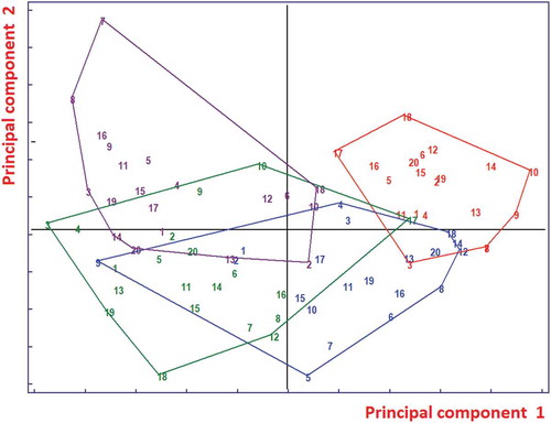
PCA shows a large overlap of the four categories. However, the first component is correlated with the order of the categories, from right for category 1 to left for category 4. The second component shows the presence of two “outliers” (objects 67 and 68 from class 4). PCA was also applied to the 14 variables autoscaled. The separation among the four classes was found to be better, especially for the first class (). It can be stated that object 57 (17 of class 3, green) is responsible for the overlap of class 3 with class 1 (red).
FIGURE 5 Correlation tree among the variables, shown as dendrogram of the similarities (correlation coefficients) obtained by means of the single linkage method. The arrow indicates the group of much correlated variables.
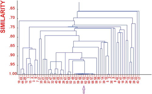
FIGURE.6 Score plot on the two first principal components of all 66 variables (autoscaled). Red: Class1, Blue: Class 2, Green: Class 3, Magenta: Class 4. The convex hulls indicate the dispersion of the classes.
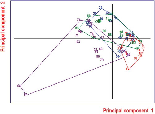
FIGURE 7 Score plot on the two first principal components of the 14 variables/features (autoscaled). Red: class 1, Blue: class 2, Green: class 3, Magenta: class 4.
Classification Analysis
The computational approaches for the classification of the freshness categories are given and discussed as follows.
LDA
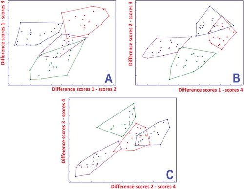
LDA was applied to the first 20 principal components of the autoscaled data that retain more than 98% of the variance. For each cancellation group, the LDA models were computed. The “canceled” objects (one-fifth) were used for prediction and others (the training set) were considered to compute the models for classification so that each object was predicted one time and classified four times. The final model was obtained with all the objects in the training set. Results indicated an excellent classification and a relatively good prediction rate. shows the results of the final model. In part A of , the difference between the scores of the objects for class 1 and those for class 3 versus the difference between class 1 and 2 separates perfectly the four classes. We also computed a prediction loss where the errors are weighed according to the distance between the real and the predicted categories, i.e., a measure of the difference between reference and predicted freshness. For instance, when a sample of class 3 is predicted in class 4, the error has weight 1; when it is predicted in class 1 the error has weight 2. Prediction loss for LDA was found
FIGURE 8 Plots of the differences between scores of LDA. Red: class 1, Blue: class 2, Green: class 3, Magenta: class 4.
KNN
KNN classifies each object according to the class of its KNN. The method was used with K = 1, 3, 5. The best results were obtained with K = 1 (1NN). In each of the five cancellation groups of cross validation, the non-canceled objects (here 64 objects) are predicted using the distances from all the other non-canceled objects (here 63 objects). In the final run, without canceled objects, each object is classified using the distance from all the remaining objects (here 79 objects). Then, each object is classified one time and predicted four times. The classification ability () of 1NN was found to be poorer than that of LDA, but the prediction ability is better (although not significantly different). Prediction loss for KNN was found to be 14.2 (KNN predicts five times, so that from the prediction matrix, the loss is computed as 71.5).
TABLE 6 Classification and prediction rates of KNN (K = 1), applied to all the autoscaled variables
QDA
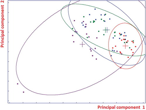
QDA needs a larger ratio of the number of objects to variables compared with LDA. Hence, it was applied to the first 15 principal components of the autoscaled data which retain about 96% of the variance. The classification ability was found to be 97.5%. This result can be explained by the fact that the space of class 1 is relatively small in comparison with the other classes. shows the QDA class spaces. The ellipses correspond to the same Mahalanobis distance from the class centroids so that almost all the objects are accepted from the model of class 4 and many objects are closest (Mahalanobis distance) to the centroid of class 4 than to the centroid of their true class in spite of a larger Euclidean distance.
FIGURE 9 95% confidence ellipses computed with T2 statistics in the space of the two first components.
Discriminant partial least squares (D-PLS)
The best results were achieved by D-PLS analysis with eight to nine latent variables (). The smallest prediction loss (i.e., 12) was found by D-PLS analysis.
TABLE 7 Classification and prediction rates of D-PLS (eight latent variables), applied to all the autoscaled variables
Results with the selections of variables
Several subsets of variables and linear transforms were checked. The best results were obtained with a combination of classification trees and LDA. Classification trees are hierarchical sequence of splitting the data set by means of binary decisions based on the values of quantitative or ordinal variables. Each decision splits the data set in two subsets. The classification trees are based on a series of splitting of the object, based on the “best” variable.[Citation23,Citation24] The linear combinations used here are LDA discriminant variables. For each combination of two categories and two variables, the LDA canonical variable was computed. For each pair of categories, the canonical variables (their number is selected by the operator) with the largest FW were selected. The result of this procedure was a set of one variable and three transforms:
The performance of the LDA model with these four features is shown in . Prediction loss for LDA decreased to 10. Hence, this is a better result both for the overall prediction ability (90%, eight errors) and for the prediction loss.
TABLE 8 Classification and prediction rates of LDA applied to the four features selected by means of multivariate classification trees
As a recommendation, the results of the current study can be coupled with innovative instruments such as electronic noses to monitor the odor of the shrimps during storage.[Citation25,Citation26] During storage, the organoleptic properties of the shrimp samples change. Therefore, odor of the stored shrimp can be gathered and injected into the sensor chamber of an electronic nose to recognize the changes accurately.
CONCLUSIONS
In this study, the potential of classification and prediction of shrimp freshness by image processing and a range of computational expert approaches was evaluated. The images captured from different parts of shrimp body were analyzed immediately after harvest and after 3, 6, and 9 days storage on ice (at a temperature of 0–4°C). The results showed high classification accuracies to recognize the freshness classes from the image parameters. In data analysis, many subsets of variables and linear transforms were checked. The best result was achieved with a combination of classification trees and LDA. Results indicated an excellent classification accuracy around 90% and a relatively good prediction rate. The computer vision system can be used for automated and online evaluation of shrimp quality and freshness. Future research could be aimed for development of a practical instrument for online monitoring and controlling shrimp storage by the use of smart phone cameras.
Acknowledgments
The authors would like to thank the support of Shahrekord University in this research.
Related Research Data
References
- Mohebbi, M.; Akbarzadeh, T.M.-R.; Shahidi, F.; Moussavi, M.; Ghoddusi, H.-B. Computer Vision Systems (CVS) for Moisture Content Estimation in Dehydrated Shrimp. Computers and Electronics in Agriculture 2009, 69(2), 128–134.
- Nollet, L.M.; Toldrá, F. Handbook of Seafood and Seafood Products Analysis; CRC Press: Boca Raton, New York, 2010.
- Rehbein, H.; Oehlenschlager, J. Fishery Products: Quality, Safety, and Authenticity; John Wiley & Sons: London, UK, 2009.
- Ghasemi-Varnamkhasti, M.; Mohtasebi, M.M.; Rodriguez-Mendez, M.L.; Gomes A. A.; Araújo, M.C.U.; Galvão, R. K.H. Screening Analysis of Beer Ageing Using Near Infrared Spectroscopy and the Successive Projections Algorithm for Variable Selection. Talanta 2012, 89, 286–291.
- Ghasemi-Varnamkhasti, M.; Forina, M.; NIR Spectroscopy Coupled with Multivariate Computational Tools for Qualitative Characterization of the Aging Of Beer. Computers and Electronics in Agriculture 2014, 100, 34–40.
- Luzuriaga, D.; Balaban, M. Evaluation of the Odor of Decomposition in Raw and Cooked Shrimp: Correlation of Electronic Nose Readings, Odor Sensory Evaluation, and Ammonia Levels. In Electronic Noses and Sensor Array Based Systems Design and Applications; Technomic: Lancaster, PA, USA, 1999.
- Dowlati, M.; de la Guardia, M.; Dowlati, M.; Mohtasebi, S.S. Application of Machine-Vision Techniques to Fish-Quality Assessment. TrAC Trends in Analytical Chemistry 2012, 40, 168–179.
- Nagalakshmi, S.A.; Mitra, P.; Meda, V.; Color, Mechanical, and Microstructural Properties of Vacuum Assisted Microwave Dried Saskatoon Berries. International Journal of Food Properties 2014, 17(10), 2142–2156.
- Nirmal, N.P.; Benjakul, S. Effect of Catechin and Ferulic Acid on Melanosis and Quality of Pacific White Shrimp Subjected to Prior Freeze–Thawing During Refrigerated Storage. Food Control 2010, 21(9), 1263–1271.
- Shafiee, S.; Minaei, S.; Moghaddam-Charkari, N.; Barzegar, M. Honey Characterization Using Computer Vision System and Artificial Neural Networks. Food Chemistry 2014, 159, 143–150.
- Sun, H.; Lv, H.; Yuan, G.; Fang, X. Effect of Grape Seed Extracts on the Melanosis and Quality of Pacific White Shrimp (Litopenaeus vannamei) During Iced Storage. Food Science and Technology Research 2014, 20(3), 671–677.
- Zhang, D.; Lillywhite, K.D.; Lee, D.-J.; Tippetts, B.J. Automatic Shrimp Shape Grading Using Evolution Constructed Features. Computers and Electronics in Agriculture 2014, 100, 116–122.
- Poonnoy, P.; Yodkeaw, P.; Sriwai, A.; Umongkol, P.; Intamoon, S. Classification of Boiled Shrimp’s Shape Using Image Analysis and Artificial Neural Network Model. Journal of Food Process Engineering 2014, 37, 257–263.
- Luzuriaga, D.A.; Balaban, M.O.; Yeralan, S. Analysis of Visual Quality Attributes of White Shrimp by Machine Vision. Journal of Food Science 1997, 62(1), 113–118.
- Du, C.; Sun, D. Comparison of Three Methods for Classification of Pizza Topping Using Different Colour Space Transformations. Journal of Food Engineering 2005, 68, 277–287.
- Brosnan, T.; Sun, D.W. Improving Quality Inspection of Food Products by Computer Vision—A Review. Journal of Food Engineering 2004, 61(1), 3–16.
- Gonzalez, R.C.; Woods, R.E.; Eddins, S. Morphological Image Processing. Digital Image Processing 2008, 3, 627–688.
- Tauler, R.; Walczak, B.; Brown, S. Comprehensive Chemometrics; Elsevier: Amsterdam, the Netherlands, 2009.
- Masniyom, P.; Benjama, O.; Maneesri, J. Extending the Shelf-Life of Refrigerated Green Mussel (Perna Viridis) Under Modified Atmosphere Packaging. Sonklanakarin Journal of Science and Technology 2011, 33(2), 171–178.
- Okpala, C.O.; Choo, W.S.; Dykes, G.A. Quality and Shelf Life Assessment of Pacific White Shrimp (Litopenaeus Vannamei) Freshly Harvested and Stored on Ice. LWT 2014, 55, 110–116.
- Huidobro, A.; López-Caballero, M.; Mendes, R. Onboard Processing of Deepwater Pink Shrimp (Parapenaeus Longirostris) with Liquid Ice: Effect on Quality. European Food Research and Technology 2002, 214(6), 469–475.
- Harper, A.M.; Duewer, D.L.; Kowalski, B.R.; Fashing, J.L. ARTHUR and Experimental Data Analysis. In Chemometrics: Theory and Applications, ACS Symposium Series 52; Kowalski, B.R.; Ed.; American Chemical Society Publisher: New York, NY, USA, 1977.
- Quinlan, R. Discovering Rules From Large Collections of Examples: A Case Study. In Expert Systems in the Micro-electronic Age; Michie, D.; Ed.; Edinburgh University Press: Edinburgh, Scotland, 1979; 168–201.
- Breiman, L.; Friedman, J.H.; Olshen, R.A. Stone, C.J. Classification and Regression Trees; Wadsworth: Belmont, CA, 1983.
- Heidarbeigi, K.; Mohtasebi, S.; Foroughirad, A.; Ghasemi-Varnamkhasti, M.; Rafiee, S.; Rezaei, K. Detection of Adulteration in Saffron Samples Using Electronic Nos. International Journal of Food Properties 2015, 18, 1391–1401.
- Dowlati, M.; Mohtasebi, S.S.; Omid, M.; Razavi, S.H.; Jamzad, M.; de la Guardia, M. Freshness Assessment of Gilthead Sea Bream (Sparus Aurata) by Machine Vision Based on Gill and Eye Color Changes. Journal of Food Engineering 2013, 119(2), 277–287.