Osmotic dehydration kinetics of banana slices considering variable diffusivities and shrinkage

ABSTRACT

This article studied the use of diffusion models to describe variation of water quantity and sucrose quantity during osmotic dehydration of bananas cut into cylindrical slices. Bananas with radius of 1.7 cm and 18 °Brix (on average) were cut into 1.0 cm of thickness. A solution was proposed for the diffusion equation in cylindrical coordinates using the finite volume method, with fully implicit formulation. The diffusion equation was discretized assuming diffusivities and dimensions with variable values for the banana slices. Boundary conditions of the third kind have also been considered. The osmotic dehydration experiments were conducted in binary solutions (water and sucrose) under conditions of 40 and 60 °Brix and temperatures of 40 and 70°C. Mathematical modeling was proposed to describe the processes presented good results for water quantity and sucrose quantity, with good statistical indicators for all fits.

KEYWORDS:

• Optimization
• Water and sucrose distribution
• Finite cylinder
• Convective mass transfer coefficient
• Effective diffusivity

Introduction

Bananas are one of the most consumed agricultural products in the world. They are rich in potassium, magnesium, and vitamin C. However, the high moisture content of the fruit contributes toward a fast deterioration of the product. Water is responsible for metabolism of bacteria and fungi which promote the decomposition of organic matter. Therefore, when the intention is to store the product or produce new products from this, such as banana passes, drying becomes an important step of the processing. In view of the importance of the drying process, various techniques have been developed.^[1,2] However, in most cases, these techniques have a high energy cost, which increases product processing cost. According to Fernandes et al.,^[3] the energy used in the drying process represents a considerable amount of all energy used by the food industry. Moreover, low thermal efficiency ranges from 25 to 50%.

Osmotic dehydration is a viable alternative to remove part of the moisture in the product and thus, reduces energy consumption. In addition to reducing the cost of the drying process, this technique brings about further gains, such as superior final products (after conventional drying). The main features of the product are highlighted by Garcia et al.^[4] These features refer to the osmotic dehydration and convective drying of pumpkins, in which osmotic dehydration causes reduction of darkening due to oxidation and acidity. They are also responsible for a decrease in the structural collapse during convective drying. As a result, the osmotic dehydration has been recommended by several authors.^[3,5–11]

Several works are found in the literature, all related to osmotic dehydration of fruits. Only a few, however, include shrinkage in the descriptions of the process.^[3,5,12,13] Notwithstanding the fact that these studies have taken into account shrinkage, none of them considers the variation of water and solids diffusivities. Nevertheless, few authors have given descriptions of osmotic dehydration considering only the variable effective diffusivity, disregarding shrinkage. Porciuncula et al.^[11] used a diffusion model, bearing in mind the geometry of a finite cylinder to determine the effective diffusion coefficient of water in banana (Prata variety) during osmotic dehydration. For modeling, only the variation of effective water diffusivity on cylindrical slices during the process was taken into account. Shrinkage was not considered. However, according to Silva et al.,^[14] to assume the variation of effective diffusivity without considering shrinkage may incur in a greater error than that of considering effective diffusivity constant. This is due to the fact that shrinkage modifies the internal structure of the product, thus affecting effective diffusivity.

Another important aspect of mass transfer in osmotic dehydration pertains to surface resistance of product mass flow. As a result, boundary condition becomes an important factor in model building, given that it can point to the surface resistance of the product so as to gain or lose mass. Monnerat et al.^[15] have observed that the plasma membrane in the plant cell wall is indeed a semi-permeable membrane that allows the passage of solvent; nevertheless, this membrane is more restrictive with respect to the passage of solutes. The main task of the convective mass transfer coefficient is to define the level of permission. Few studies, however, have considered boundary condition of the third kind to describe the mass transfer processes during osmotic dehydration.^[16,17] The aim of this article is to make a description of the osmotic dehydration process of banana slices considering some unusual cases found in the literature. In the modeling developed, the shrinkage of banana cylinders during the process, the variation of water and sucrose diffusivities, and the boundary condition of the third kind have been considered.

Material and methods

Mathematical modeling

In the present study, diffusion models are used to describe mass transfer in the banana osmotic dehydration process. Moreover, the following factors have been taken into account: the product bears the geometry of a finite cylinder, it shrinks and the mass diffusivities vary along the whole process. In order to consider the product’s resistance to mass flow on its surface, a boundary condition of the third kind has been assumed.

Diffusion equation

Each banana sample was regarded as a finite cylinder with radius R and length L. In this case, the diffusion equation is given by:^[18]

(1)

where represents water or sucrose quantity (%), as rules the case, represents effective mass diffusivity (water or sucrose), represents a transport coefficient (in this study ), r and y are the position coordinates (Fig. 1b) and t is the time. In order to numerically solve the diffusion equation, Eq. (1), the following assumptions have been accepted:

• The finite cylinder has radius R and length L.

• The cylinder is homogeneous and isotropic.

• The spatial distribution of quantities of interest within the cylinder has radial and axial symmetries.

• Diffusion is the only mass transport mechanism within the cylinder.

• The cylinder radius and the length vary during diffusion.

• Effective mass diffusivities vary during osmotic dehydration, and the convective mass transfer coefficients remain constant.

Figure 1. A: Symmetrical slice to the cylindrical geometry; B: Two-dimensional grid with the boundaries east (E), west (W), north (N), and south (S), with a grid element highlighted; C: Internal control volume and neighbors to the north (N), south (S), west (W) and east (E); and D: Northeast volume control and neighbors to the west and south.

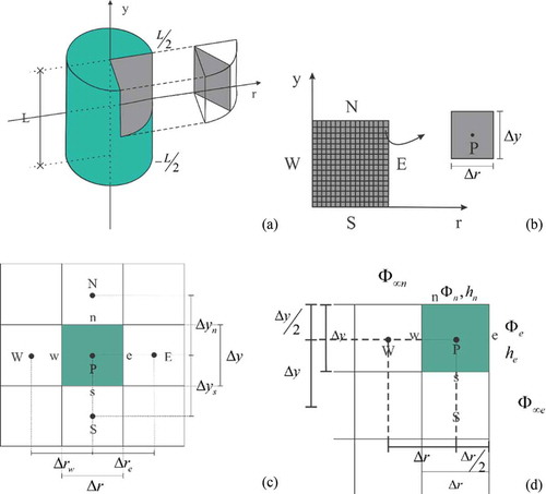
Considering the hypothesis of symmetry, a two-dimensional domain is obtained as shown in Fig. 1a and 1b. Consequently, only half of the cylinder is analyzed, saving considerable processing time and computer memory.

Discretization of the diffusion equation

Equation (1) was discretized by applying the finite volume method^[19] using a fully implicit formulation. By integrating Eq. (1) in space and in time , we obtain the following semi-discretized equation (Eq. [2]):

(2)

where the superscript “0” of the quantity of interest shows that this quantity may be assessed at the beginning of the time interval, the subscript “e,” “w,” “n,” and “s” are, respectively, the east, west, north, and south interfaces; while P is the nodal point of the volume control.

Discretization for internal control volumes

Internal control volumes have no contact with external medium. They have four neighboring control volumes: one north, one south, one west, and one east, as shown in Fig. 1c. Considering the derivatives approaches with respect to interfaces north, south, east, and west for a uniform grid ( and ), we obtain the following discretized equation:

(3)

where

(4)

(5)

(6)

(7)

(8)

(9)

It is worth observing that Eq. (3) is an algebraic equation obtained by discretization of the partial differential equation given through Eq. (1). The dependent variable for the control volume P is and for its neighbors to east, west, north, and south are , , , and , respectively. On the other hand, , , , , and , as well as B, are coefficients of the algebraic equation.

Discretization for the northeast control volume

The northeast control volume is in contact with the external medium to the north and east, and has neighboring control volumes to the west and south, as shown in Fig. 1d. In Fig. 1d, and are the values of the quantity of interest on the eastern and northern boundaries, respectively; and and represent the equilibrium quantity of interest in the external medium to the east and to the north, respectively. Considering the equality of convective and diffusive fluxes on the boundaries to the north and east, and the approaches of derivatives on the western and southern boundaries, we obtain:

(10)

where

(11)

(12)

with and given by Eqs. (6) and (8). The parameters and are the convective mass transfer coefficients referent to the boundaries north and east, respectively.

The discretization of the other seven types of control volumes is obtained analogously to those which have been presented so far. In this discretization, one should consider the zero fluxes to west and south. As the present study considers the variation of the product dimensions at every instant of time, the values of and are updated depending on the water or sucrose quantities (depending on each case).

Validation and numerical solution convergence

In the case of finite cylinder, the whole implicit formulation provides, at every time interval, a system of linear equations. To solve these linear system, we used the method TDMA-Gauss (Tridiagonal Matrix Algorithm-Gauss) Seidel combination.^[19] This method was used to reduce the computational cost of the Gauss-Seidel method. The Gauss-Seidel method was used with a convergence tolerance of. In order to validate the numerical solution, such solution was compared to an analytical solution. The validation process revealed that the results provided by the numerical solution were equivalent to those provided by the analytical solution.

Average value of the quantity of interest

At each time instant, the numerical solution gives the value of the quantity of interest at each nodal point. As the contributions to each volume control for the average value are not the same, the average value of quantity of interest, at every time instant, is obtained by calculating the weighted average:

(13)

where .

Parameter assessment

Considering the hypotheses to obtain the numerical solution, the diffusion equation was discretized assuming that the parameter may vary in relation to the local value of the quantity of interest, for example:

(14)

where a and b are coefficients of a function that fit the numerical solution to the experimental data, and are determined by optimization. Considering the discretization presented, one needs to know the parameter at the interfaces of all control volumes. In the case of value at the nodal points, this is calculated by means of Eq. (14), at every step of the optimization process. To calculate at the interface between the control volume P and E, for instance, the following expression is used:^[19]

(15)

Optimization

In order to obtain the process parameters (a, b, h) using experimental datasets, an optimizer was coupled to the numerical solution. This optimizer was also used by Silva et al.,^[14] where initial values are assigned to the parameters, and then these are corrected in order to minimize the objective function (here, the chi-square function). The values of convective mass transfer coefficients and (Fig. 1d) were considered equal (), since both surfaces are of the same kind and have been submitted to the same experimental conditions.

Experimental data on osmotic dehydration of bananas

The banana used in the osmotic dehydration experiments was the Manzano bananas. The fruit belongs to the AAB genomic group, acquired in the local market (Campina Grande PB, Brazil) at fourth stage of maturity: yellower than greener—according to the using Von Loesecke scale.^[20] On being acquired, the bananas were kept at room temperature until they reached the last stage of maturation: yellow with brown areas.

Before starting the osmotic dehydration experiments, the fruits were washed in tap water, sanitized with chlorinated water for a period of 15 min. They were finally washed again with water and peeled manually. The fruits were then sliced in cylindrical pieces of approximately 1.0 cm in length and 1.7 cm in radius. The average moisture content of the samples was 3.090 (db). After being sliced, the samples were separated, weighed, and put in baskets, which were grouped in triplicate and, finally, labeled.

The solution used in the osmotic dehydration process was that of the binary type, distilled water and commercial sucrose, prepared at the ratio of 1:15 (g/g; of fruit for solution) at concentrations of 40 and 60 °Brix. The ratio used aimed to keep unchanged concentrations during the experiments. Osmotic dehydration experiments were performed using a combination of concentrations of 40 and 60 °Brix with temperatures of 40 and 70°C. These experimental conditions were selected because of existing studies, where the temperatures range from 25–70°C and concentrations range from 30–70 °Brix.^[3,7,11,12]

The monitoring of the kinetics of water quantity and sucrose quantity was conducted according to the methodology described by Silva et al.^[21] Samples in triplicate were labeled (representing the time when the samples were withdrawn from the solution). In addition to these samples, one sample was used in triplicate to verify the shrinkage each time, measuring the diameter and length of each repetition. In order to obtain expressions to describe shrinkage under all experimental conditions, data were turned into dimensionless values by using the following equations:

(16)

where and are the dimensionless values of the radius and length, respectively, at time ; and are the values (in meters) of the radius and length, respectively, at time ; and are the values (in meters) of the radius and length, respectively, at time . Table 1 shows the calculated values for the equilibrium water quantity, equilibrium sucrose quantity, initial radius and the initial length for each experimental condition. To calculate in percentage the water quantity in the product at each time t, the following formula was used:

(17)

Table 1. Osmotic dehydration temperature (T), concentration of the solution, equilibrium water quantity (), equilibrium sucrose quantity (), initial radius of the cylinder (, and initial height of the finite cylinder ().

T (°C)	Concentration (° Brix)			(m)	(m)
40	40	53.70	25.33
40	60	30.01	28.49
70	40	23.16	50.69
70	60	17.90	58.13

where is the percentage water quantity in the product at time t, is the mass of the sample n₁₁ at time t, is the mass of the sample n₁₁ at time zero, is the dry mass of the sample n₁₁ at time t and is the dry mass of the sample n₁₁ at time zero. To calculate the sucrose quantity incorporated (in percentage) at time t over the initial dry mass, the following formula was used:

(18)

where is the percentage sucrose quantity in the product at time t.

Results and discussion

The optimization process and simulation were carried out by considering grid with 30 × 20 control volume and 2000 time steps. These numbers were obtained after a study considering different configurations of grid and time steps. Radius and length variations have been described in relation to the quantities water and sucrose. For such, all dimensionless shrinkage data were analyzed by LABFit Software,^[22] which provided the following fits:

(19)

where represents the average water quantity at time t. Analogous fits were made considering the shrinkage data based on the quantity of sucrose. The following expressions were obtained:

(20)

where is the average sucrose quantity incorporated at time t. Several expressions were tested for the effective water diffusivity depending on the local water quantity. Of all the expressions tested the one with the best statistical indicators was as follows:

(21)

Using Eq. (21) for the effective water diffusivity and the expression of Eq. (19) for shrinkage, the optimizations carried out produced the results shown in Table 2. The results shown in Table 2 demonstrate that the modeling developed in the present work was suitable for describing variation of water quantity during osmotic dehydration. In all optimizations implemented, the value of the convective mass transfer coefficient (h) was very high, demonstrating that the most suitable boundary condition is that of the first kind. The works that consider the variable effective diffusivity in osmotic dehydration are but a few. Porciuncula et al.^[11] used an exponential expression and a linear expression to represent the variation of effective water diffusivity in osmotic dehydration of banana. The exponential expression was found to be far more suitable. Both expressions were tested during the present work optimization processes, but they did not have the best statistical indicators. In the present study, 30 expressions were carefully tested. Furthermore, Porciuncula et al.^[11] did not consider the possibility of shrinkage, but according to Silva et al.,^[14] to assume the variation of effective diffusivity without considering shrinkage can cause a far greater error than that incurred when considering the effective diffusivity constant.

Table 2. Results for the optimizations of water quantity and water sucrose.

		Obtained values
Experimental conditions	Parameters/statistical indicators	Water quantity	Water sucrose
40 °Brix and 40°C	a
	b
	h
	R^2	0.9900	0.9982
	χ^2	20.0681	1.1282
60 °Brix and 70°C	a
	b
	h
	R^2	0.9973	0.9955
	χ^2	19.0368	16.5495
40 °Brix and 70°C	a
	b
	h
	R^2	0.9984	0.9973
	χ^2	9.3403	7.0136
60 °Brix and 40°C	a
	b
	h
	R^2	0.9945	0.9933
	χ^2	25.7295	5.5077

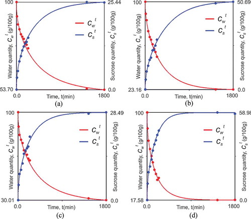
Figure 2 shows the fits for water quantity under four experimental conditions. As the statistical indicators in Table 2 had already exhibited, the fit shown in Fig. 2 suggest that the modeling developed to describe variation of water quantity during the osmotic dehydration process was acceptable. As shown in Fig. 2d, one can see that in middle of the process time, equilibrium value is already reached. This shows that under the experimental conditions of 60 °Brix and 70°C, the processing time for water loss can be minimized, getting closer to 900 min. Figure 2 still shows that the temperature and the concentration of the solution have influenced the equilibrium water quantity. However, temperature has influenced more significantly than concentration. Such impacts have been further considered in other works on osmotic dehydration.

Figure 2. Kinetics of water quantity and sucrose quantity obtained for the experimental conditions: A: 40 °Brix and 40°C; B: 40 °Brix and 70°C; C: 60 °Brix and 40°C; and D: 60°Brix and 70°C.

Atares et al.,^[12] when investigating the impact of solution concentration and temperature on the final quality of the banana, concluded that both concentration and temperature had no significant effect on the equilibrium value of mass loss. However, the equilibrium values were obtained by these authors with Peleg equation, since the experiments extended for only 4 h. Mercali et al.^[23] identified the influence of temperature, sucrose concentration and NaCl concentration on the equilibrium moisture content during osmotic dehydration of bananas. However, as evidenced by Atares et al.,^[12] the equilibrium moisture content was obtained with Peleg equation. Moreover, the experiments were conducted for only 10 h. As the equilibrium values shown in Fig. 2 were obtained experimentally, these results may be considered more appropriate.

Figure 3a depicts the strong influence of temperature and concentration on the whole process. This was also observed in the following works: Fernandes and Rodrigues,^[5] Singh et al.,^[24] and Abraão et al.^[25] Singh et al.^[24] observed the important influence exerted by temperature and immersion time on the water loss; however, according to the authors, the effect of osmotic solution concentration was not significant in relation to water loss.

Figure 3. A: Water quantity simulations for the four experimental conditions; B: Sucrose quantity simulations for the four experimental conditions; and C: Effective water diffusivity as a function of the local water quantity for the four experimental conditions.

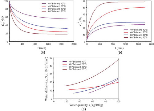
Similar to the present work, Fernandes and Rodrigues^[5] have observed the influence of both temperature and concentration on the water loss in osmotic dehydration experiments in ternary solutions. However, the NaCl concentration was far more influential than temperature. Finally, also in Fig. 3a, one notices that after about 1000 min, the equilibrium is nearly reached in all experimental conditions. This information is useful to decide when is the best time to remove the product from within the binary solution.

As can be seen in Fig. 3c, the effective water diffusivity goes up as the local water quantity increases. Moreover, conversely, it is observed that as the product loses water during the process, the effective diffusivity decreases. This is due to the fact that the water present in the product is more concentrated in the lower layer; as a result, the resistance to such water is conveyed to the upper layers becomes larger. It should also be noted that in an osmotic dehydration process there occurs the incorporation of solids, which may contribute to the increased resistance to water loss. This fact has also been observed by Singh et al.^[24]

Still, Fig. 3c is observed at a concentration of 60 °Brix and the increase in temperature caused led to the increase effective diffusivity and at temperatures of 40 to 70°C the increase in the concentration also led to the increased effective diffusivity. One can also see that effective diffusivity increases with an increase in temperature (at a concentration of 60 °Brix) and in concentration (at temperatures of 40 and 70°C). Using the same grid and the same number of time steps used in water quantity optimizations and the expressions of Eq. (20), optimizations were performed to improve sucrose quantity. The best expression found for the effective sucrose diffusivity was as follows:

(31)

where is the effective sucrose diffusivity, and represents the local sucrose quantity at time . The optimization results are shown in Table 2. Silva et al.^[21] performed osmotic dehydration experiments on guava immersed in binary solutions (water and sucrose), and the mathematical modeling developed included a variation of diffusivities. Among several tested expressions, the one with the best statistical indicators for the effective sucrose diffusivity was a variation of the expression found in this study. It can also be said that in both studies effective sucrose diffusivity presented similar behavior. Further studies should be conducted to determine which would be the best expression to describe the effective sucrose diffusivity; whether the expression should be related to the product or to the experiment. As in the case of water quantity, the statistical indicators presented indicate a good description of the process gain sucrose.

Figure 2 shows the fits for the sucrose quantity under all four experimental conditions. As it occurred regarding the variation of water quantity as shown in Fig. 3b, one can see that at about half of processing time, equilibrium is reached. Therefore, under the experimental conditions of 60 °Brix and 70°C, the processing time for sucrose gain can be shorter, close to 900 min. In order to analyze the influence of temperature and concentration on sucrose quantity, in Fig. 2b the kinetics for the four experimental conditions have been arranged. As it happened to water quantity, both the temperature and the concentration had an impact on the sucrose quantity. However, temperature has had an influence slightly higher than the concentration in all cases studied. These results were also obtained by other authors: Singh et al.,^[26] Mundada et al.,^[27] Uribe et al.,^[28] Arballo et al.,^[29] and Abraão et al.^[25] Finally, still on Fig. 2b, one has observed that after about 800–1000 min the equilibrium is reached for practically all experimental conditions.

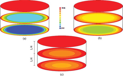
In order to verify the behavior of the water and the sucrose quantity on the product, Figs. 4 and 5 illustrate the distributions of the water and sucrose quantities on circular surfaces (from the center of the cylinder to the top). This analysis was made in view of the experimental conditions of 40 °Brix and 70°C. These distributions refer to the circular surfaces of the cylinder center, of the top and in the surface located to 1/4 of the center in time t = 180 min, t = 450 min, and t = 900 min.

Figure 4. Water quantity distribution in the circular surfaces of the cylinder center, of the top and in the surface located to 1/4 of the center (40 °Brix and 70°C): A: t = 180 min; B: t = 450 min; and C: t = 900 min, where the number 100 of the scale represents the initial water quantity and 23.2 represents the equilibrium water quantity.

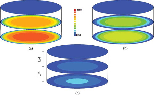
Figure 5. Sucrose quantity distribution in the circular surfaces of the cylinder center, of the top and in the surface located to 1/4 of the center (40 °Brix and 70°C): A: t = 180 min; B: t = 450 min; and C: t = 900 min, where the number 0 of the scale represents the initial sucrose quantity and 50.6 represents the equilibrium sucrose quantity.

As expected (and indicated in Fig. 4), the water loss occurs from the middle to the top of the cylinder; consequently, the central surface of the cylinder holds greater water quantity along the three times studied. This is due to the fact that the surface in contact with the external environment loses water at a much faster rate. As the values obtained for h had already revealed, the top of the cylinder is already in equilibrium with the environment after 180 min from the beginning of the process. However, after 900 min the cylinder center has not yet reached its equilibrium.

Conversely to what occurred in the water loss, the sucrose gain developed from the surface to the center (Fig. 5); as result the central surface has the least sucrose quantity along the three times being studied. Due to boundary condition, the top of the cylinder is already in equilibrium with the environment after 180 min from the beginning of the process. However, after 900 min the center of the cylinder has not yet reached equilibrium.

Conclusion

The model developed in the present study proved to be most appropriated to describe the variation of water quantity and sucrose quantity in the banana osmotic dehydration process. The temperature and solution concentration had an impact on the water quantity and on the sucrose quantity. However, temperature has had an influence slightly higher on water quantity and sucrose quantity than the concentration. In all experimental conditions, h leans toward infinity. This clearly indicates a boundary condition of the first kind. However, such a far more general modeling can be applied to studies on osmotic dehydration of other products, which can present surface resistance to mass transfer. During the water loss, it has been observed that after about 1000 min the equilibrium was reached in all experimental conditions. Since the gain of sucrose, it was observed that after about 800–1000 min equilibrium is reached for practically all experimental conditions.

Nomenclature

	=	Coefficients of the discretized diffusion equation
a, b	=	Fitting parameters
	=	Local water quantity at the instant t (g/100 g)
	=	Local sucrose quantity at the instant t (g/100 g)
	=	Equilibrium water quantity (g/100 g)
	=	Equilibrium sucrose quantity (g/100 g)
h	=	Convective mass transfer coefficient ()
L	=	Height of the finite cylinder ()
	=	Initial height of the finite cylinder ()
	=	Dimensionless height
	=	Radius of the cylinder ()
	=	Initial radius of the cylinder ()
	=	Dimensionless radius
	=	Coefficient of determination (dimensionless)
	=	Thickness of a control volume ()
	=	Transport coefficient ()
	=	Dependent variable of the diffusion equation (g/L00g)
	=	Chi-square or objective function (dimensionless)

Funding

Wilton Pereira da Silva would like to thank the Conselho Nacional de Desenvolvimento Científico e Tecnológico (CNPq) for the support given to this research and for his research grant (Processes Number 302480/2015-3 and 444053/2014-0).

Additional information

Funding

Wilton Pereira da Silva would like to thank the Conselho Nacional de Desenvolvimento Científico e Tecnológico (CNPq) for the support given to this research and for his research grant (Processes Number 302480/2015-3 and 444053/2014-0).

References

- Demiray, E.; Tulek, Y. Degradation Kinetics of β-Carotene in Carrot Slices during Convective Drying. International Journal of Food Properties 2016. DOI:10.1080/10942912.2016.1147460
- López-Vidaña, E.C.; Figueroa, I.P.; Cortés, F.B.; Rojano, B.A.; Ocaña, A.N. Effect of Temperature on Antioxidant Capacity During Drying Process of Mortiño (Vaccinium Meridionale Swartz). International Journal of Food Properties 2016. DOI:10.1080/10942912.2016.1155601
- Fernandes, F.A.N.; Rodrigues, S.; Gaspareto, O.C.P.; Oliveira, E.L. Optimization of Osmotic Dehydration of Bananas Followed by Air-Drying. Journal of Food Engineering 2006, 77, 188–193.
- Garcia, C.C.; Mauro, M.A.; Kimura, M. Kinetics of Osmotic Dehydration and Air-Drying of Pumpkins (Cucurbita Moschata). Journal of Food Engineering 2007, 82, 284–291.
- Fernandes, F.A.N.; Rodrigues, S. Ultrasound as Pre-Treatment for Drying of Fruits: Dehydration of Banana. Journal of Food Engineering 2007, 82, 261–267.
- Lewicki, P.P.; Kamińska, A. Diffusion of Sucrose in Osmo-Dehydrofrozen Apple. International Journal of Food Properties 2015, 18, 2110–2123.
- Mercali, G.D.; Marczak, L.D.F.; Tessaro, I.C.; Noreña, C.P.Z. Evaluation of Water, Sucrose and NaCl Effective Diffusivities During Osmotic Dehydration of Banana (Musa Sapientum, Shum.). LWT–Food Science and Technology 2011, 44, 82–91.
- Mohebbi, M.; Shahidi, F.; Fathi, M.; Ehtiati, A.; Noshad, M. Prediction of Moisture Content in Pre-Osmosed and Ultrasounded Dried Banana Using Genetic Algorithm and Neural Network. Food and Bioproducts Processing 2011, 89, 362–366.
- Oliveira, I.M.; Fernandes, F.A.N.; Rodrigues, S.; Sousa, P.H.M.; Maia, G.A.; Figueiredo, R.W. Modeling and Optimization of Osmotic Dehydration of Banana Followed by Air Drying. Journal of Food Process Engineering 2006, 29, 400–413.
- Pereira, N.R.; Marsaioli Jr., A.; Ahrné, L.M. Effect of Microwave Power, Air Velocity and Temperature on the Final Drying of Osmotically Dehydrated Bananas. Journal of Food Engineering 2007, 81, 79–87.
- Porciuncula, B.D.A.; Zotarelli, M.F.; Carciofi, B.A.M.; Laurindo, J.B. Determining the Effective Diffusion Coefficient of Water in Banana (Prata Variety) During Osmotic Dehydration and Its Use in Predictive Models. Journal of Food Engineering 2013, 119, 490–496.
- Atares, L.; Gallagher, M.J.S.; Oliveira, F.A.R. Process Conditions Effect on the Quality of Banana Osmotically Dehydrated. Journal of Food Engineering 2011, 103, 401–408.
- Dehghannya, J.; Gorbani, R.; Ghanbarzadeh, B. Shrinkage of Mirabelle Plum during Hot Air Drying as Influenced by Ultrasound-Assisted Osmotic Dehydration. International Journal of Food Properties 2016, 19, 1093–1103.
- Silva, W.P.; Silva e Silva, C.M.D.P.; Farias, V.S.O.; Gomes, J.P. Diffusion Models to Describe the Drying Process of Peeled Bananas: Optimization and Simulation. Drying Technology 2012, 30, 164–174.
- Monnerat, S.M.; Pizzi, T.R.M.; Mauro, M.A.; Menegalli, F.C. Osmotic Dehydration of Apples in Sugar/Salt Solutions: Concentration Profiles and Effective Diffusion Coefficients. Journal of Food Engineering 2010, 100, 604–612.
- Silva, W.P.; Silva, C.M.D.P.S.; Lins, M.A.A.; Gomes, J.P. Osmotic Dehydration of Pineapple (Ananas Comosus) Pieces in Cubical Shape Described by Diffusion Models. LWT–Food Science and Technology 2014, 55, 1–8.
- Silva, W.P.; Silva, C.M.D.P.S.; Junior, A.F.S. A Numerical Approach to Determine Some Properties of Cylindrical Pieces of Bananas During Drying. International Journal of Food Engineering 2015, 11, 335–347.
- Luikov, A.V. Analytical Heat Diffusion Theory. Academic Press, Inc. Ltd.: London, 1968; 685 pp.
- Patankar, S.V. Numerical Heat Tranfer and Fluid Flow. Hemisphere Publishing Cooperation: New York, NY, 1980; 197 pp.
- Pbmh and Pif—Programa Brasileiro para a Modernização da Horticultura & Produção Integrada de Frutas [Brazilian Program for the Modernization of Horticulture & Integrated Fruit Production]. Normas de Classificação de Banana. São Paulo: CEAGESP, 2006.
- Silva, W.P.; Aires, J.E.F.; Castro, D.S.; Silva, C.M.D.P.S.; Gomes, J.P. Numerical Description of Guava Osmotic Dehydration Including Shrinkage and Variable Effective Mass Diffusivity. LWT–Food Science and Technology 2014, 59, 859–866.
- Silva, W.P.; Silva, C.M.D.P.S. LAB Fit Curve Fitting Software, V.7.2.46, 2009. www.labfit.net (accessed 24 April, 2015).
- Mercali, G.D.; Tessaro, I.C.; Noreña, C.P.Z.; Marczak, L.D.F. Mass Transfer Kinetics During Osmotic Dehydration of Bananas (Musa Sapientum, Shum.). International Journal of Food Science and Technology 2010, 45, 2281–2289.
- Singh, B.; Panesar, P.S.; Nanda, V. Osmotic Dehydration Kinetics of Carrot Cubes in Sodium Chloride Solution. International Journal of Food Science and Technology 2008, 43, 1361–1370.
- Abraão, A.S.; Lemos, A.M.; Vilela, A.; Sousa, J.M.; Nunes, F.M. Influence of Osmotic Dehydration Process Parameters on the Quality of Candied Pumpkins. Food and Bioproducts Processing 2013, 91, 481–494.
- Singh, B.; Panesar, P.S.; Nanda, V.; Kennedy, J.F. Optimisation of Osmotic Dehydration Process of Carrot Cubes in Mixtures of Sucrose and Sodium Chloride Solutions. Food Chemistry 2010, 123, 590–600.
- Mundada, M.; Hathan, B. S.; Maske, S. Mass Transfer Kinetics During Osmotic Dehydration of Pomegranate Arils. Journal of Food Science 2011, 76, 31–39.
- Uribe, E.; Miranda, M.; Vega-Gálvez, A.; Quispe, I.; Clavería, R.; Di Scala, K. Mass Transfer Modelling During Osmotic Dehydration of Jumbo Squid (Dosidicus Gigas): Influence of Temperature on Diffusion Coefficients and Kinetic Parameters. Food Bioprocess Technology 2011, 4, 320–326.
- Arballo, J.R.; Bambicha, R.R.; Campañone, L.A.; Agnelli, M.E.; Mascheroni, R.H. Mass Transfer Kinetics and Regressional-Desirability Optimisation During Osmotic Dehydration of Pumpkin, Kiwi and Pear. International Journal of Food Science and Technology 2012, 47, 306–314.