A new method for accurate, high-throughput volume estimation from three 2D projective images

ABSTRACT

In this article, a new method for estimating the volume of selected fruits and vegetables, using information obtained from three orthogonal images of the object is proposed. The method was based on a novel lower bound on this volume, combined with an application of a well-known upper bound. The lower bound was obtained by calculating the volume of an artificial object created from the intersection of the three object silhouettes. The method was applied to a significant range of food products and simple geometric objects, and it was found that the method estimated volume with approximately 11.9% error, generally, and 2%, for rounded objects, specifically.

KEYWORDS:

• High throughput
• Biomass
• Phenotyping
• Upper and lower bounds
• Volume estimation

Introduction

One of the most immediate and revealing properties of any olericultural, viticultural, and pomological product is volume. The volume of food products gives an indication of produce quality, growth behaviour, economic value, and physiological defects.^[1] When combined with weight, one can estimate average density, which provides important information on water content, biomass,^[2,3] consistency, and flavour.^[4] The density of fruit can be used to detect the presence of hidden effects such as frost damage.^[5,6] On the other hand, if the density of the product is assumed to be approximately constant, then an estimation of product volume also enables to determine product weight, which is also a valuable phenotypic trait.^[7,8]

In a commercial context, where high-throughput food production and, hence, quality control are paramount to ensure a streamlined distribution pipeline, a rapid, accurate, and non-destructive means of determining food product volume is important.^[9] High-resolution imaging is becoming an important scientific tool in plant biology generally as it can be used to quantify plant phenotype,^[10–12] and plant response to environmental stresses^[13] in terms of changes in development, growth rate, and crop yield. The natural question to ask is whether, in the horticultural context, one can also obtain accurate estimates of volume with images. This is the focus of this article. The approach proposed in this article can be also used in medical imaging, where detecting and tracking the volumetric growth of tumours in an organ over time is critical for the identification of abnormalities and, consequently, for accurate diagnoses.^[14,15]

The volume of an object can be accurately estimated given its 3D shape, reconstructed using multiple images from different viewpoints. From a computer vision perspective, several techniques have been proposed for reconstructing 3D shapes of objects from multiple images. Examples include multiview stereo,^[16] shape from shading, structured light, and shape from silhouettes, also known as the visual hull.^[17] Accurate 3D reconstruction using these methods, however, requires many images, typically more than 10 taken from different perspectives, and efficient and accurate camera calibration. This reduces the flexibility of these methods and their usability by non-experts. It also makes them impractical for high-throughput volume and biomass estimation. In fact, existing high-throughput phenotyping facilities generally only acquire two or three orthogonal views of each object, which makes accurate 3D reconstruction challenging.

Many techniques estimate 3D volume by incorporating prior knowledge about the object to utilize some relationship between the volume and the 2D properties measured.^{[1,4,6,15,18–22]} While these methods provide quick and easy ways of obtaining volume estimates, they are limited in the range of objects that can be analysed and do not facilitate automated analysis of different types of objects. A completely different approach was proposed in^[23,24], where the statistics of different geometric properties of the 2D projections is used to classify each object. While this technique is appealing since all information is obtained from the 2D projections, it requires a large number of images. The closest method to the one proposed in this article was introduced by Wulfsohn et al.^[25] Their method creates a support function using sampled points from a 2D projection of an axially convex object. Using a number of projections from different angles and the Cavalieri principle,^[26] the authors obtain accurate estimates for the true volumes of potatoes, parsnips, and bananas. Similar to^[27], the accuracy depends on the number of views used in the estimation.

In this article, a new method for volume estimation is proposed. The technique estimates the volume directly from only three orthogonal images without explicit 3D reconstruction of the object’s shape. The proposed approach makes no assumption about the shape of the object, except that it is convex, axially symmetric, and axially aligned. From these images, estimates of both upper and lower bounds of the true volume are obtained. The results presented here show that the average of the estimated upper and lower bounds provides a very accurate estimate of the true volume. The method is compared with other methods, such as the visual hull^[17] as an upper bound, the lower bound estimates provided by the convex hull,^[27,28] and the volume estimation of Wulfsohn et al.^[25]

Materials and methods

Materials

The approach proposed here was applied to eight different fruits and vegetables (carrot, potato, tomato, orange, capsicum, lime, apple, and pear), and to eight artificial objects with known volume (sphere, cube, ellipsoid, bipyramid, cylinder, bicone, rectangular prism, and triangular prism), in order to further validate the approache’s accuracy. Images of the fruits and vegetables were captured using a three-image acquisition system. Each object was carefully positioned so as to adhere to the assumption of axial alignment. The cameras used were PointGrey and Flea2 RGB colour cameras with 8 mm lenses. They were placed at approximately equal distances from the scene centre and orthogonal to each other. A uniform background was set behind the object in order to facilitate the foreground–background subtraction process.

Methods

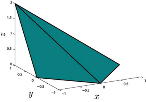
The main assumptions are required that the objects under consideration are convex, that the principal axes of these convex objects are aligned with the projection axes during acquisition, and that the objects are approximately symmetric about the -axis. Wulfsohn et al.^[25] noted that many sorting machines capable of aligning objects axially are nowadays commercially available. Furthermore, many common fruits and vegetables are approximately axially symmetric. Figure 1 shows an example of an object (a square pyramid) that would not be suitable for volume estimation using the proposed approach. Here, the square pyramid’s apex is tilted away from the objects centre. Hence, the object is not symmetric about the -axis and would produce a misleading 2D projection in the plane, resulting in a construction that overestimates the object’s true volume.

Figure 1. Example of an object that is not axially symmetric and hence not applicable for use with the proposed approach. The object here is a pyramid whose base forms a square centred at (0,0,0) in the x-y plane and the apex has been tilted to the position (-1,1,2).

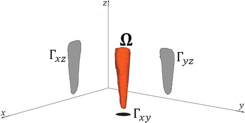
Let be a three-dimensional convex body. Denote its projections onto the three orthogonal coordinate planes, and , by and , respectively, as shown in Fig. 2. Let and , respectively, denote the boundaries of these regions. To estimate the volume, , of the object, from the shape and size of its projections, the areas, , and , of the projections are used. The aim is to establish an upper bound, , and a lower bound, , on the true volume of the object ,using only three 2D projections of , such that:

(1)

Figure 2. A representation of a typical configuration of a convex body, Ω, (in this case an actual carrot), with its three projections, Γ_xy, Γ_xz and Γ_yz, in the three orthogonal coordinate planes.

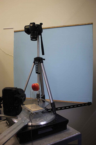
and is as close as possible to the true volume of V. The complete process for determining the volume estimate, is displayed in Fig. 3. All image processing steps and volume calculations were undertaken in Matlab 2012a. First, the objects are imaged so as to capture the three orthogonal coordinate projections, the imaging setup is shown in Fig. 4. Next, the images are segmented using colour thresholding, so that all object pixels are classified as foreground and all other pixels are classified as background. The boundaries of the foreground objects are then obtained using the Moore-Neighbor tracing algorithm. Finally, the segmented objects and their boundary points were used to calculate the upper and lower bounds on the object’s true volume.

Figure 3. Pipeline of the complete volume estimation process. After the images are acquired they are segmented and the object’s boundary is extracted. The segmented object and its boundary are subsequently used to determine the upper and lower bound on the true volume.

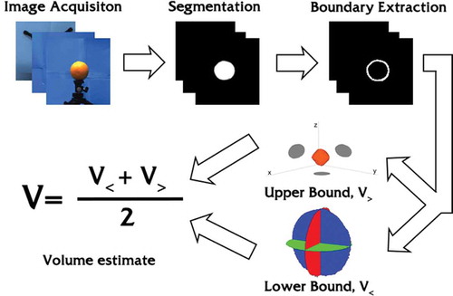
Figure 4. The imaging setup used to obtain the three orthogonal views of the object, in this case an apple. The camera is rotated around the turntable to capture the x-z and y-z projections. The tripod is placed on the turntable to capture the x-y projection, and then removed for horizontal image capture.

An upper bound on volume

Loomis and Whitney^[29] considered upper bound estimates of the volume of a convex body using only the areas of its orthogonal projections. Their analysis was very general, and they considered an abstract -dimensional object, , with distinct (−1)-dimensional projections, for . Here, their result, valid specifically for the 3D case, is utilized, which is

(2)

where are the areas of the three projections. This method assumes nothing about the object in question except for convexity and only requires computation of the areas of the 2D orthogonal projections, hence making it simple to use and also suitable for the high-throughput scenario. The challenge now lies in finding an easily computable lower bound on the volume that effectively negates the error of this upper bound when the two are averaged together, resulting in an accurate estimation of the object’s true volume.

A lower bound on volume

The novel approach proposed in this article is based on finding the volume of a new object, , created from the three orthogonal projections of an object, , but whose volume is less than that of . This object is found by aligning the projections so that the centre of mass of the projection is at the origin of the 3D coordinate frame and the widest sections of the and projections are centred vertically at and horizontally at and , respectively. This alignment is demonstrated in Fig. 5, for the cases of an orange and a carrot. Note that in some cases, for instance, that of a regular pyramid, the object will reside only on or above the plane. Finally, the boundaries of these translated projections are connected with a surface distribution of straight lines.

Figure 5. (a) Orange. (b) Carrot. Aligned projections of a fruit and a vegetable. The dark projection is from the x-y plane while the two lighter projections are from the x-z and y-z planes.

Connecting the boundaries of these translated projections with a surface distribution of straight lines, analogous to stretching a thin film over a wire frame, produces a closed 3D, but not necessarily convex body, whose volume will be less than that of . Figure 6 shows how the straight lines are connected and how the quantitative construction is used to estimate the volume of the new object would proceed.

Figure 6. Schematic showing one octant of the minimum convex body Ω’ and two typical wedges for determining volume, one wedge is shown on either side of the break point (x_b,y_b,0).Variables that contribute to the calculation of volume, Eq. (4), are indicated.

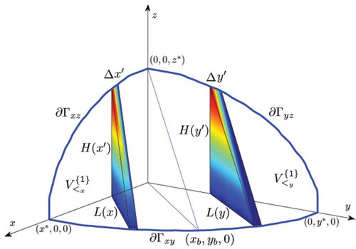
A point on one boundary, say , is connected by straight lines to two unique points on one orthogonal boundary ( or ). As points on trace that boundary from the coordinate plane, say, , the point’s unique connecting points on the closest orthogonal boundary, here , trace the latter boundary until the apex of at is reached, identifying a unique “break” point on , From then on, points on possess two straight line connections that trace the boundary from the apex to the extreme point on the x-axis, . When deciding upon an appropriate break point, one faces the task on choosing a trade-off between accuracy and efficiency. Optimization algorithms can be used to find the optimal break point but greatly decrease the speed of the algorithm. On the other hand, simply choosing the centre point of as the break point is much faster and results in no great loss of accuracy. This construction suggests that diamond-shaped objects such as bicones and bipyramids are very well represented by the new object, and thus, their volumes will be accurately estimated (please note later that the diamond symbols in Figs. 9 and 10 were purposely chosen to reflect this feature).

Figure 7. (a) Sample images prior to background-foreground separation of approximately convex fruit and vegetables. Left - orange, center - capsicum, right - carrot. (b) The purpose-built pycnometer used to determine volumes of irregularly shaped objects. An apple is visible in the device.

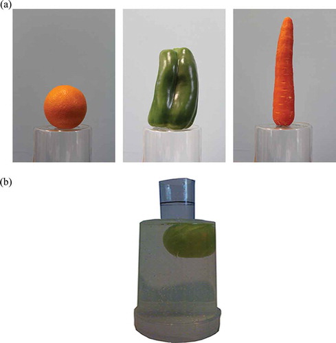
Figure 8. A comparison of true and upper and lower estimated volumes for the objects listed in Table 1, ordered according to increasing true volume. Curves lying under the 45° line are lower bound estimates with the curve marked with triangles representing our approach and the curve marked with addition symbols the convex hull; curves lying above this line are upper bound estimates with the curve marked with circles representing the Loomis Whitney upper bound and the curve marked with squares representing the visual hull.

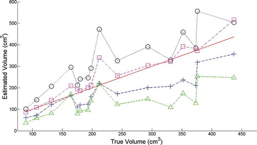
Figure 9. A comparison between true and estimated volumes for the objects listed in Table 1. Open circles represent the V_UL estimates; filled diamonds are V_<; filled squares are V_>.

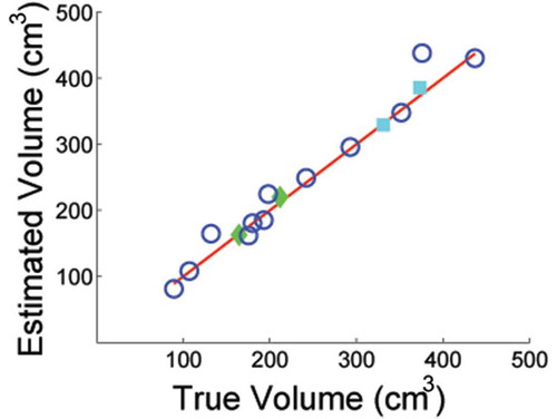
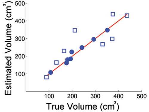
Figure 10. A comparison of true and estimated volumes as a function of object shape. Solid circles refer to high curvature objects; open squares refer to low curvature objects. All symbols are V_UL results.

For illustrative purposes, the description of volume calculations is limited to that section of that lies in the positive octant, that is, for points , and . The volume calculations for the other seven octants follow immediately, and the volume of is then the sum of all eight octant contributions. First, the part of that lies between the break point and the plane is discretized into segments. Similarly, the interval on the -axis from 0 to is discretized with a -mesh and a series of wedges of base length , height , and perpendicular width are constructed. The base of a given wedge extends from a given discrete point on to its corresponding point on the -axis . The height is the -component of the point on directly above . The wedge width, , depends on the discretization of the -axis through the relation . The remainder of is similarly discretized, this time for points that connect to unique points and on the -axis and , respectively. Thus, a series of wedges of width are formed. Figure 6 shows two wedges, one on either side of the break point and the relationship between the quantities.

The volumes of each wedge of the two discrete sets are calculated and summed to give the total volume of this octant’s contribution to . Summing over all wedges on one side of the break point provides an approximation to the volume of that section of the octant, using the formula for the volume of parallel-sided triangular prisms. Namely,

(3)

A corresponding result, , is obtained for the remaining part of the octant. Summing the quantities and gives the total volume of the octant . This expression estimates volume while requiring only information from the object’s projections. Note also that this construction uses volumetric slices of the 3D body and hence is analogous to an integral over the entire body. It may be possible that using this formulation, a simple closed form expression for the volume, relying only on area (much like the Loomis–Whitney bound), can be found. This gratuity is something not found in many methods used for volume estimation such as the visual and convex hulls.

Volume estimation

The two previous sections focused on expressions for lower and upper bounds of an object’s true volume, each based only on the object’s orthogonal projections. Although one hopes that either one (or both) would give a sufficiently accurate estimate of the volume, they are, by definition, less reliable in terms of providing exact measures of volume. On the other hand, an average of the upper and lower bounds can give an even better approximation to an object’s true volume than could either bound itself. Consequently, one of the principal findings of this work was to utilize the average of the lower and upper bound:

(4)

for just this purpose. This method was validated using numerical examples and applied to real fruit and vegetables in the Results and Discussion section.

Other approaches

In this section, some alternate approaches for estimating upper and lower bounds of volumes are reviewed. In the Results and Discussion section, they will be compared to the approach proposed in this article as well as to the upper bound from Loomis and Whitney.

A lower bound from Makeev^[28]

Makeev proposed an approach where a lower bound on the total volume can be estimated from each of the three projections individually, with the maximum estimate over the three projections being chosen as the most accurate lower bound. In this approach, the largest line parallel to the -axis contained in the projection of the convex body is used to construct a cone with apex and base at either end of the line. The authors show that the volume of this cone is less than or equal to the volume of the convex body.

The visual hull^[17]

Three-dimensional shape from silhouettes is a popular technique for 3D reconstruction. The method relies on the availability of multiple images acquired from different viewpoints. From each captured image, the object of interest, hereafter referred to as the foreground, is segmented from the background, thus creating a silhouette. Each silhouette is prescribed a virtual 3D cone whose apex is at the camera centre and whose sides pass through the silhouette point boundary. The visual hull of the object is defined to be the intersection of all such 3D cones based on the silhouettes obtained from the different camera viewpoints. Geometrically, the visual hull is the closest shape to the real object that can be reconstructed from the silhouettes.

The convex hull

Given a set of points in three-dimensional space, the convex hull of the set is defined as the smallest convex polyhedron that contains all points. If the object in question is assumed to be convex, then the convex hull takes the form of the smallest object possible given the point set. While the visual hull gives the closest possible upper bound on the volume of the object, the convex hull gives the closest possible lower bound on the volume of a convex object.

An estimate from Wulfsohn et al.^[24]

Here, the authors use planar cuts of a number of 2D projections of the object, and the Cavalieri principle,^[26] in order to gain an estimate on the volume of axially convex objects. Like the visual hull, this approach becomes more accurate with a larger number of sample images. The approach does not guarantee a lower or upper bound on the object but rather an estimate of its exact volume.

Validation

For the fruit and vegetable items shown in Fig. 7a, a pycnometer^[3] was used to measure volume after imaging. The device, shown in Fig. 7b, has a removable, sealable base and a long, narrow top. An object is weighed (O) and then placed inside the device via the base and sealed. The device is then filled with water from the top. The long, narrow top prevents the object from floating above the water line.

The volume is given by:

(5)

where is the density of water; , and are, respectively, the weight of the pycnometer containing Water only, the weight of the Object, and the weight of the pycnometer containing Both the object and water. The combination gives the mass of displaced water. All objects were weighed on a digital scale accurate to ±1 gm. An estimate of the error associated with a pycnometer volume measurement was obtained for the case of a simple geometric object, a sphere. The pycnometer volume was compared to the sphere’s geometric volume, . The sphere’s diameter, , was measured using a set of digital vernier calipers, accurate to ±0.01 mm. The geometric volume was found to be 514.22 . Using the pycnometer, the volume was found to be 514 , providing us with a percentage error of approximately 0.04%.

For the case of geometric objects, the true volume values were calculated from geometric formulae using random values (in mm) for the essential parameters such as sphere radius and pyramid height. The advantages of these cases were that they were readily applicable to the upper and lower bound estimates.

Results and discussion

In this section, the volume formulae given in Eqs. (2)–(4) are compared with exact results for one of each type of fruit, vegetable, and simple geometric object. These will represent target items for application of the proposed method. To evaluate the performance of the proposed method, the results are compared with the previously described approaches: the visual hull, the Makeev lower bound, the convex hull, and the method of Wulfsohn et al. (2004).

To convert silhouette information from image coordinates in pixels to real-world coordinates in units of length (mm’s), one of the three cameras was chosen as reference, (e.g., the camera providing the projection). The camera’s distance to the scene center is then measured to an acceptable accuracy. As all cameras image the same object, the and , images are re-scaled to correspond to the image. This simulates the configuration where all cameras are placed at equal distances from the object centre without relying on accurate calibration. Finally, using the focal length and camera centre of the first camera ( plane), all three silhouettes are converted from pixels to units of length.

Table 1 summarizes the true and estimated volume data for all objects. Of this dataset, the individual upper and lower estimates are represented graphically in Fig. 8, plotted against true volume. Perfect correspondence is represented by the 45 line. This figure and the ideal 45 line highlight two features. First, the concepts of upper and lower bounds are appropriately represented, being above and below the 45 line, respectively. Second, the figure highlights the relative performance of the two sets of upper and lower bounds. The lower bound, , being closer to the ideal line, performs generally better than Makeev’s approach, Eq. (7). The few instances where both perform well reflect the nature of the shape being modelled. This was fully anticipated given the relationship between the shapes and the way that the bounds were derived. The upper bounds also performed surprisingly well, with the Loomis–Whitney model performing worse than the visual hull, which is known to give good upper estimates of volume, but also recognized to be labour intensive and time-consuming.

Table 1. True volumes obtained by manual measurement and results of volume estimations.

	Object	True Vol.	Lower Bound (this work)	Upper bound (Loomis and Whitney)	Mean	Visual Hull	Makeev	Convex Hull	Wulfsohn
Fruit and vegetables	Carrot	132	107.39	206.89	157.14	142.27	82.26	136.52	140.23
	Potato	242	162.4	326.37	244.39	257.00	122.62	209.42	257.19
	Tomato	180	119.02	240.59	179.81	186.58	93.35	151.4	179.66
	Orange	293	197.75	390.93	294.34	304.02	147.93	238.49	289.35
	Capsicum	437	321.5	649.95	485.73	516.39	247.69	476.75	483.75
	Lime	107	69.34	144.26	106.8	108.91	59.27	91.02	120.61
	Apple	193	138.43	246.55	192.49	201.13	96.35	154.16	192.05
	Pear	198	166.06	290.7	228.38	212.65	141.18	194.75	186.76
Geometric Shapes	Sphere	351.97	230.74	459.48	345.11	392.48	173.5	272.62	345.47
	Cube	373.25	190.95	385.9	288.43	382.36	128.7	317.15	329.88
	Ellipsoid	175.41	107.05	213.46	160.26	194.58	80.22	127.47	156.84
	Bipyramid	278.88	277.23	472.77	375.00	340.61	219.09	227.31	344.80
	Cylinder	89.17	45.74	101.88	73.81	86.15	37.51	75.75	91.863
	Bicone	173.62	168.66	295.9	232.28	208.77	169.87	173.04	187.90
	Rectangular Prism	331.20	165.55	329.63	247.59	322.24	109.96	274.06	284.78
	Triangular Prism	375.89	179.18	556.7	367.94	372.31	253.23	351.3	513.289

The results, shown in Fig. 9, represent the principal findings of this article. The average, , provides an accurate estimate of volume over a wide range of sizes and shapes. This fact is demonstrated by the circle symbols, which lie along the ideal 45 line. In those few instances where performed less well, either the upper bound, , or the lower bound, , individually, gave an accurate estimate of the true volume. The filled symbols represent those estimates (diamonds for the lower bound and squares for the upper bound). In these instances, the values of are not shown.

Clearly, there are cases where the average performs very well, while both lower or upper bound estimates individually perform poorly. There are also cases where one or other of the upper or lower bounds individually performs very well, and performs poorly. To elicit a rationale for these trends, which might guide the creation of an automatic way of choosing which mode to apply for the best possible result, the different cases can be distinguished from one another. Close inspection of the objects tested for which performs well reveals that most are round objects, such as apples and oranges. On the other hand, there are clear cases where performs well, such as the cube, cylinder, and rectangular prism. Then, there are cases where performs best, such as the carrot, bi-pyramid, the bi-cone, and triangular prism. The second point to note is that these cases are mutually exclusive: There is no instance when any two bounds perform well. Clearly, the object’s overall geometry is an important factor. Consequently, we have categorized objects according to their mean solid angle curvature. Let and be the local principal curvatures, then the mean solid angle curvatures, and , of an object are defined to be:

(6)

In Eq.(6), the summation is over disjoint volumetric regions , partitioned by surface contours along which the local curvatures are undefined. The differential of the solid angle is , where and are the polar and azimuthal spherical polar angles, respectively. Using Eq (6), three classes of objects can be defined; those of high mean solid angle curvature, when neither nor is zero; those of low mean solid angle curvature, when one of or is zero; and those that are piece-wise flat, when . For convenience, this latter case is included in the low mean solid angle curvature category. Thus, only two classes need be considered. Examples of objects with high mean solid angle curvature are spherical and ellipsoidal objects, and this includes many common fruits and vegetables such as apples, oranges, and potatoes. Objects with low mean solid angle curvature include cubes and rectangular prisms. While the mean solid angle curvature measure proposed here is not a unique identifier of objects, (e.g., consider the mean solid angle curvatures of a cone with a spherical cap) it is useful for quantitatively discerning between spherical and ellipsoidal objects, and all other objects.

Figure 10 presents the same results as shown in Fig. 9 but separated into the classes of high and low mean solid angle curvature objects. Generally, for high curvature objects, the average, , performs very well, with an average error of only 1.92%. For low curvature objects, the sub-classification of bi-prismoidal and cubical is necessary to account for the mutually exclusive performances of and . By design, the lower bound naturally does better for objects that are bi-prismoidal, while the Loomis–Whitney upper bound, gives a more accurate account of cubical objects. These three mutually exclusive trends can be used to select the appropriate estimate to apply in any given case. As can be seen in Table 2, when the bi-prismoidal and cubical objects are removed from the error calculations, the average error over all objects drops from 11.86% to 1.92%.

Table 2. The average error of each method, given as a percentage, for all objects and then for only high-curvature objects.

		Convex hull	Visual hull	Wulfsohn
Avg. error for all objects	11.86%	16.65%	7.06%	9.6%
Avg. error for high curvature objects	1.92%	23.82%	5.57%	4.7%

As expected, the convex hull provides a lower bound that is too accurate to be used in conjunction with the desirable Loomis–Whitney upper bound. On average, the Loomis–Whitney upper bound produces 139% of the true volume; hence, the convex hull which gives on average approximately 83.35% of the volume is less suitable than the novel lower bound proposed in this article, which gives 68.71% of the true volume.

Timing

All computations were run on a desktop PC Intel Core2 Duo CPU with 2.53 GHz processor speed. The novel method proposed in this paper has a processing time of approximately 0.3 s for geometric shapes and approximately 0.4 s for actual fruit/vegetable shapes. The convex hull required, on average, 0.18 s, while the visual hull took longer than 2 s in all cases, in addition to the tedious and time consuming camera calibration step.

Conclusion

In this article, a means of estimating volumes of convex objects based only on information derived from three orthogonal images is proposed. The method is based on determining upper and lower bounds of the object volume, expressed in terms of the areas of the object’s three silhouettes. An extensive comparison between physically measured volumes and volume estimates obtained with the average, , is performed and results show that over a significant range of volumes and shapes, estimates object volumes with only 11.9% error and approximately 2% error when the scope of objects studied is limited to spherical and ellipsoidal shapes. Hence, the method’s performance can be categorized in terms of object curvature. For objects that have a very low value for at least one of their principal curvatures (e.g., a cylindrical shaped object), the Loomis–Whitney upper bound does very well on its own. On the other hand, volumes of objects that are bi-prismoidal in shape are more reasonably estimated by . For objects whose two principal curvatures are comparable, gives a good estimate of true volume. In the latter case, the upper and lower bound estimates compensate for each other’s deficiencies. The main finding of this work is that a fast, accurate, and simple means of estimating volume, particularly for high curvature objects such as oranges and apples, is available in , which requires only knowledge of three orthogonal 2D projections. Costly 3D reconstruction is not required, which makes this approach better suited for large scale, high-throughput quality control, and phenotyping. A challenging extension of this work is to consider a generalization to non-convex objects, with arbitrary orientation.

Acknowledgments

The authors would like to thank Dr. Jorge Aarao for valuable discussions.

Funding

This project is supported with funding from the Grains Research and Development Corporation, Australia.

Additional information

Funding

This project is supported with funding from the Grains Research and Development Corporation, Australia.

References

- Ngouajio, M.; Kirk, W.; Goldy, R. A Simple Model for Rapid and Nondestructive Estimation of Bell Pepper Fruit Volume. HortScience 2003, 38(4), 509–511.
- Miller, W.M.; Peleg, K.; Briggs, P. Automatic Density Separation for Freeze-Damaged Citrus. Applied Engineering in Agriculture 1988, 4, 344–348.
- Forbes, K. Volume Estimation of Fruit from Digital Profile Images. Master’s thesis. University of Cape Town 2000.
- Omid, M.; Khojastehnazhand, M.; Tabatabaeefar, A. Estimating Volume and Mass of Citrus Fruits by Image Processing Technique. Journal of Food Engineering 2010, 100(2), 315–321.
- Iqbal, S.M.; Gopal, A.; Sarma, A.S.V. Volume Estimation of Apple Fruits Using Image Processing. International Conference on Image Information Processing 2011, 1–6.
- Forbes, K.A.; Tattersfield, G.M. Estimating Fruit Volume from Digital Images. Africon 1999, 1, 107–112.
- Roman, I.; Ardelean, M.; Mitre, V.; Mitre, I. Phenotypic, Genotypic and Environmental Correlations between Fruit Characteristic Conferring Suitability to Juice Extraction in Autumn Apple. Horticulture 2007, 64(1–2), 760.
- Düzyaman, E.; Düzyaman, B.Ü. Fine-Tuned Head Weight Estimation in Globe Artichoke (Cynara scolymus L.). HortScience 2005, 40(3), 525–528.
- Salmanizadeh, F.; Nassiri, S. M.; Jafari, A.; Bagheri, M. H. Volume Estimation of Two Local Pomegranate Fruit (Punica granatum L.) Cultivars and Their Components Using Non-Destructive X-Ray Computed Tomography Technique. International Journal of Food Properties 2015, 18(2), 439–455.
- Paproki, A.; Sirault, X.; Berry, S.; Furbank, R.; Fripp, J. A Novel Mesh Processing based Technique for 3D Plant Analysis. BMC Plant Biology 2012, 12(1), 1–13.
- Cai, J.; Miklavcic, S.J. Automated Extraction of Three-Dimensional Cereal Plant Structures From Two Dimensional Orthographic Images. IET Image Processing 2012, 6, 687–696.
- Chopin, J.; Laga, H.; Huang, C.Y.; Heuer, S.; Miklavcic, S.J. RootAnalyzer: A Cross-Section Image Analysis Tool for Automated Characterization of Root Cells and Tissues. PloS One 2015, 10(9), e0137655.
- Roy, S.J.; Tucker, E.J.; Tester, M. Genetic Analysis of Abiotic Stress Tolerance in Crops. Current Opinion in Plant Biology 2011, 14(3), 232–239.
- Popa, T.; Ibanez, L.; Levy, E.; White, A.; Bruno, J.; Cleary, K. Tumor Volume Measurement and Volume Measurement Comparison Plug-ins for Volview using ITK. Proceedings of the SPIE: The International Society for Optical Engineering 2006, 6141, 395–402.
- Feldman, J.; Goldwasser, R.; Mark, S.; Schwartz, J.; Orion, I. A Mathematical Model for Tumor Volume Evaluation Using Two-Dimensions. Journal of Applied Quantitative Methods 2009, 4(4), 455–462.
- Seitz, S.M.; Curless, B.; Diebel, J.; Scharstein, D.; Szeliski, R. A Comparison and Evaluation of Multi-View Stereo Reconstruction Algorithms. Proc. 2006 IEEE Conference on Computer Vision and Pattern Recognition 2006, 1, 519–528.
- Laurentini, A. The Visual Hull Concept for Silhouette-Based Image Understanding. IEEE Transactions on Pattern Analysis and Machine Intelligence 1994, 16, 150–162.
- Banta, L.; Cheng, K.; Zaniewski, J. Estimation of Limestone Particle Mass from 2D Images. Powder Technology 2003, 2(24), 184–189.
- Khojastehnazhand, M.; Omid, M.; Tabatabaeefar, A. Determination of Tangerine Volume Using Image Processing Methods. International Journal of Food Properties 2010, 13(4), 760–770.
- Vivek Venkatesh, G.; Iqbal, S.M.; Gopal, A.; Ganesan, D. Estimation of Volume and Mass of Axi-symmetric Fruits Using Image Processing Technique. International Journal of Food Properties 2014, 18(3), 608–626.
- Ziaratban, A.; Azadbakht, M.; Ghasemnezhad, A. Modeling of Volume and Surface Area of Apple from Their Geometric Characteristics and Artificial Neural Network (ANN). International Journal of Food Properties 2016 (DOI: 10.1080/10942912.2016.1180533).
- Yous, S., Laga, H., Kidode, M., Chihara, K. GPU-based Shape Frome Silhouettes. Proceedings of the 5th International Conference on Computer Graphics and Interactive Techniques in Australia and Southeast Asia; Association for Computing Machinery: New York, USA, 2007, 71–77, 207.
- Presles, B.; Debayle, J.; Cameirao, A.; F´evotte, G.; Pinoli, J. Volume Estimation of 3d Particles with Known Convex Shapes from Its Projected Areas. 2nd International Conference on Image Processing Theory, Tools and Applications 2010, 399–404.
- Presles, B.; Debayle, J.; Pinoli, J.C. Size and Shape Estimation of 3-d Convex Objects from Their 2-d Projections: Application to Crystallization Processes. Journal of Microscopy 2012, 248, 140–155.
- Wulfsohn, D.; Gundersen, H.J.G.; Jensen, E.B.V.; Nyengaard, J.R. Volume Estimation from Projections. Journal of Microscopy 2004, 215, 111–120.
- Daintith, J.; Nelson, R.D.; Eds. The Penguin Dictionary of Mathematics; Puffin Books: City of Westminster, London, UK; 1989.
- Bradford Barber, C.; Dobkin, D.P.; Huhdanpaa, H. The Quickhull Algorithm for Convex Hulls. ACM Transactions on Mathematical Software 1996, 22(4):469–483.
- Makeev, V.V. On Approximation of a Three-Dimensional Convex Body by Cylinders. St. Petersburg Math. Journal 2006, 17, 315–323.
- Loomis, L.H.; Whitney, H. An Inequality Related to the Isoperimetric Inequality. Bulletin of the American Mathematical Society 1955, 55, 961–962.