Variability of Cole-model bioimpedance parameters using magnitude-only measurements of apples from a two-electrode configuration

ABSTRACT

Electrical impedance measurements have been widely researched to monitor physiological changes in fruits and vegetables in a nondestructive manner. Recently, the parameters of the Cole bioimpedance model (R₀, R₁, C, and α), an equivalent circuit that is widely used to represent the electrical impedance of biological tissues, were extracted using techniques without direct impedance measurements. In this study, the variability of the Cole parameters extracted from magnitude-only measurements (from 200 Hz to 1 MHz) of apples in a two-electrode setup was examined to understand the impact of electrode placement on the parameters evaluated using this technique. Eight electrodes were placed around the center latitudinal line of apples to collect seven sets of measurements from four different varieties (Granny Smith, Fuji, Red Delicious, and Spartan). The Cole impedance parameters were extracted in MATLAB from the collected measurements using a nonlinear least squares fitting method. These extractions indicated that the parameters R₀ and R₁ had the highest variability based on the electrode location, whereas the dispersion coefficient (α) had the lowest variability.

KEYWORDS:

• Bioimpedance
• Cole-model
• Apples

Introduction

Nondestructive methods, including ultrasonic spectroscopy^[1] and visible/near infrared spectroscopy,^[2] have previously been investigated to estimate the properties of fruits, vegetables, and other food products. Another technique used to monitor physiological changes in biological tissues is impedance spectroscopy, which quantifies the resistance of a material to an injected electrical stimulus.^[3] These measurements have recently been investigated to monitor fruits and vegetables in a nondestructive manner^[4] for various applications, such as quantifying damage to apples;^[5] determining drying and freezing/thawing effects on eggplant samples;^[6] measuring durian dry matter content to classify maturity;^[7] monitoring pressure-induced changes of carrots, potatoes, and red radishes^[8]; detecting the nitrogen status of lettuce;^[9] characterizing the cell vitality loss of Shiraz berries during ripening;^[10] assessing the storage shelf life of refrigerated squid;^[11] classifying mangosteen flesh translucency^[12]; investigating the impact of air drying on the dehydrofreezing of carrots^[13]; and measuring strawberry ripeness.^[14] In applications that monitor the electrical impedance of tissues, the two analysis techniques most widely used are the following: (1) evaluating changes in electrical impedance at discrete frequencies (either singular or multiple frequencies) collected at different times and (2) evaluating changes in the parameters of an equivalent electrical circuit that represents the full electrical impedance datasets collected at different times.

When applying the equivalent electrical circuit method, components with a fractional-order impedance have been widely used in various models.^[15] These fractional-order components can be broadly defined with an impedance Z_F = Fs^α, where F is the fractance and α is the order, with s^α = (jω)^α = ω^α[cos(απ/2) + jsin(απ/2)]. The introduction of α represents the import of concepts from fractional calculus,^[16,17] the branch of mathematics concerning noninteger differentiation and integration, into electrical circuit theory. When applying fractional calculus to electrical circuit theory, the traditional elements (capacitors, resistors, and inductors) are viewed as special cases of the general fractance with a fixed order (α = −1, 0, 1, respectively). In biology, another special case referred to as a constant phase element (CPE) is widely used. This element has an impedance Z_CPE = 1/s^αC, where C is a pseudo-capacitance with units F s^α−1. These devices have also been called fractional-order capacitors, in reference to their order (α), which takes a value between the traditional circuit elements of a resistor and capacitor. It is for this reason that a capacitor is used as the schematic representation of CPEs in this work. A CPE is often used as a component in a simple circuit model to represent the impedance of biological tissues. This model, given in Fig. 1a, is known as the Cole impedance model or often the Cole bioimpedance model, with an impedance given by

(1)

Figure 1. (a) Theoretical Cole impedance model to represent experimentally collected data from biological tissues. (b) Simple circuit to collect magnitude response using Cole impedance as a component.

This model is composed of three hypothetical circuit elements, resistors R₀ and R₁ and a CPE (C, α). The Cole impedance model is widely used due to its simplicity and good fit with measured data, illustrating the behavior of impedance as a function of frequency. The studies presented in Refs.^[18,19] have shown that large three-dimensional resistor/capacitor (RC) networks are well represented by fractional-order models, supporting the use of (1) to represent the behavior of biological tissues, which can be viewed as complex 3D structures of cells, each with their own resistance and capacitance that are based on intercellular, intracellular, and cellular membrane properties.

The circuit parameters that represent the impedance of a biological tissue are typically determined using direct impedance measurements, which require both the magnitude and phase of the fruit or vegetable to be measured. However, previous works have investigated the extraction of these parameters without direct impedance measurements using only the magnitude response^[20,21] or step response^[22] to reduce the hardware complexity and determine the impedance by eliminating the requirement of measuring the phase response (for magnitude methods) or generating sinusoidal test signals (for time-domain methods). However, although these previous methods have verified the accuracy of using the magnitude response to extract the circuit parameters,^[20,21] no studies have explored the variability of parameters extracted from the same fruit using different electrode positions. Understanding this impact will be an important consideration for applications in which measurements collected at different times may have different electrode locations as a result of transport processes as well as for comparing the results from studies with different electrode locations. Understanding the impact of electrode position will also provide reference ranges for the minimum level of change required to assess whether physiological changes (such as ripening, bruising, or infection) are captured by changes in the extracted parameters or are artifacts of variability in electrode location.

This study examined the variability of Cole impedance parameters (R₀, R₁, C, and α) extracted using an indirect, magnitude-only measurement technique with varying electrode locations in a two-electrode configuration. The remainder of this article is organized as follows. Introduction section introduces the Cole impedance model and its applications, with the circuit theory, experimental setup, and nonlinear least squares fitting (NLSF) process for parameter extraction described in Materials and methods section. The NLSF process is applied to the experimental data collected from 20 apples of 4 different varieties using 7 electrode pairs with the extracted parameters presented in Result section. The article closes with a discussion of these results and outlines future research in Discussion section.

Materials and methods

The Cole impedance model has previously been used as a component in a filter^[20] and integrator circuit topology^[23] for measuring the resulting magnitude response. From these collected magnitude responses, the Cole impedance parameters (R₀, R₁, C, and α) were numerically calculated from direct measurements^[20,23] or by using a NLSF routine.^[24] Here, a similar approach is applied to collect the magnitude response when an apple is used as the Cole impedance in a simple filter circuit, shown in Fig. 1b. In this figure, v_in is the sinusoidal input voltage and v_o is the corresponding output voltage across the load resistor R_L. The transfer function of this circuit is given by

(2)

with the magnitude response of Eq. (2) expressed as

(3)

where X₀(ω) = 1 + ω^α CR₁cos(απ/2), X₁(ω) = 1 + ω^αCR₁sin(απ/2), X₂(ω) = R₀ + R₁ + R_L + ω^αCR₁(R₀ + R_L)cos(απ/2), and X₃(ω) = ω^αCR₁(R₀ + R_L)sin(απ/2). There are three distinct regions based on the magnitude response given by Eq. (3): (1) when the CPE is approximated as an open circuit (Z_CPE ≈ ∞) at low frequencies close to DC, the response is constant, yielding a magnitude of |H(ω ≈ 0)|= R_L/(R₀ + R₁ + R_L); (2) an increasing-magnitude region resulting from the decrease in CPE impedance; and (3) when the CPE behaves as a short circuit (Z_CPE ≈ 0) at high frequencies, the response is again a constant value with magnitude |H(ω≈∞)|= R_L/(R₀ + R_L). This overall response can be considered as a high-pass type filter, with its greatest attenuation at low frequencies and its minimum attenuation at high frequencies.

Measurement system

The magnitude response of each apple in this study was collected using the test setup given in Fig. 2. In this setup, the apple was used as the Cole impedance in Fig. 1b with a load resistor R_L = 992 Ω. The sinusoidal input and output voltages were generated and measured, respectively, using an Agilent 4395A network analyzer configured to collect the transmission (B/R) measurements.

Figure 2. Experimental test setup to collect magnitude response using Agilent 4395A network analyzer when an apple is used as a component in a simple filter circuit.

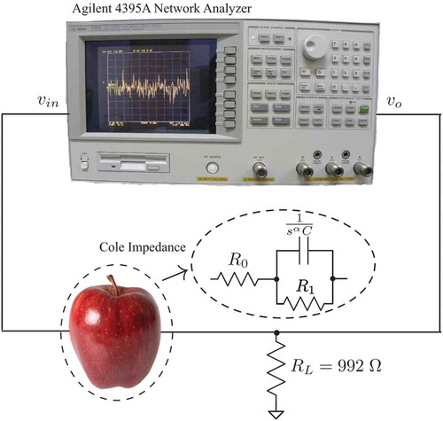
For simplicity, 22 AWG solid copper wire was used as the electrodes to interface each apple with the measurement circuit, with each wire inserted to a depth of 10 mm. Measurements were collected using seven electrode arrangements, with the top and side views of the electrode-insertion locations shown in Fig. 3. For each measurement, only two electrodes were inserted into the sample being tested, with the input signal applied to locations labeled “Electrode 1,” “Electrode 2,” … “Electrode 7” and measured at the “reference electrode” location. The dotted line in the side view of Fig. 3 corresponds to the latitudinal position around each apple at which the electrodes were placed. For these measurements, it was assumed that the damage to the tissue resulting from the insertion of the electrode had a negligible impact on the collected data. A two-electrode setup was selected over a four-electrode configuration to simplify the test circuit and explore the variability in the test system that could be implemented most easily.

Figure 3. Top and side views of electrodes placed into apples for collection of magnitude responses.

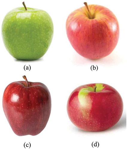
Magnitude responses were collected from four varieties of apples (Granny Smith, Fuji, Red Delicious, and Spartan), with examples of each type shown in Figs. 4a–4d. Each variety possesses different shapes, flavors, and textures and could potentially have different variabilities based on physiological differences. The electrical impedance of apples has previously been investigated to determine the relationships between the major parameters that contribute to taste^[25] and for quality assessment to detect bruising^[5]. However, neither study explored the variability in impedance based on electrode location, and both used a four-electrode measurement method.

Figure 4. (a) Granny Smith, (b) Fuji, (c) Red Delicious, and (d) Spartan varieties of apples.

Each variety of apples for this study was selected because of its widespread availability in Canadian supermarkets and was purchased from a local grocer in Calgary, Canada. These apples were all selected to be similar in size, with no visible bruising or breaks in the surface. Before collecting any measurements, the apples were placed in the laboratory for 24 h at a temperature of approximately 23°C.

Results

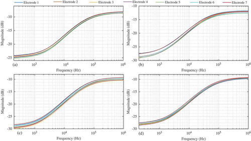
The collected magnitude responses from 200 Hz to 1 MHz when R_L = 992 Ω for one Granny Smith apple, one Fuji apple, one Red Delicious apple, and one Spartan apple are shown in Figs. 5a–5d, respectively. Each figure has seven sets of data labeled electrode 1–7 corresponding to the dataset using that electrode and the reference electrode, as detailed in Fig. 3. Each dataset displays the characteristics predicted by Eq. (3), with the largest attenuations (reaching as low as −30 dB) occurring at 200 Hz and the minimum attenuations (reaching as high as −10 dB) occurring at 1 MHz. The most visible differences between the responses of each apple are the gains at low and high frequency. This difference is most clearly highlighted in the Fuji datasets of Fig. 5b when comparing electrode pairs 1–2 (with low-frequency gains of approximately −27.5 dB) to pairs 3–7 (with low-frequency gains of approximately −29 dB). These data illustrate that electrode placement does indeed impact the collected magnitude response.

Figure 5. Magnitude responses collected from a single (a) Granny Smith, (b) Fuji, (c) Red delicious, and (d) Spartan varieties of apples using different electrode configurations.

Nonlinear least squares extraction

Although multiple techniques are available to extract the Cole impedance parameters,^[26,27] the NLSF numerical method described in Ref.^[28] was used in this work. This method was applied to extract the single-dispersion Cole impedance parameters (R₀, R₁, C, α) that describe the data in Fig. 5, as opposed to the double-dispersion parameters from Ref.^[28] This routine attempted to find the impedance parameters that ideally reduced the least squares error (LSE) between a simulated response using Eq. (3) and the experimental data to zero but realistically reduces it to the level of noise within the dataset. This process to minimize the LSE is described as

(4)

where x is the set of impedance parameters (R₀, R₁, C, α) to minimize f₀(x), |H(x,ω_j)|is the magnitude response given by Eq. (3) at frequency ω_j, y_j is the measured magnitude response at frequency ω_j, and n is the total number of measured data points. The constraints (x > 0) were added to the problem because negative resistances and capacitances are not physically possible, and a negative α would indicate fractional-order-inductive characteristics, which were not considered in this study. This NLSF was implemented in MATLAB using the lsqcurvefit function configured to terminate searching when any of the following conditions was satisfied: (1) the number of function evaluations exceeded 5000; (2) the number of iterations of the algorithm exceeded 5000; (3) the change in the value of x was less than 10⁻¹⁰; or (4) the change in the function value was less than 10⁻¹⁰.

First, the lsqcurvefit implementation of this NLSF required an initial iterate, x₀, be supplied to begin the search, then iteratively solving from x₀ toward the unknown solution x*. After quitting due to meeting any of the ending criteria, the solver returns a possible solution. However, many local minima may exist that satisfy the ending criteria without being the true global solution for this problem. Therefore, the solver has the potential to return solutions that are not the true impedance parameters. One method to overcome this problem requires executing the solver multiple times using a different initial iterate on each execution^[28]. The intent is to generate an initial starting condition that is highly similar to the global solution such that the solver returns the global solution when the ending criteria are met, avoiding any local minimum. Therefore, solving Eq. (4) from each x₀ and selecting the solution that yields the lowest LSE increases the likelihood of finding the global solution. For the analysis in this study, the solver was applied 20 times to each dataset with a new initial condition generated for each execution. These initial conditions were randomly generated using the rand function in MATLAB within the ranges 0.1 Ω < R_0,1 < 10 kΩ, 10 µF < C < 0.1 F, and 0 < α < 1. After the 20 executions, the parameter set with the lowest LSE was selected as the solution set (x*). Although multiple search algorithms exist for NLSF, the available options for the lsqcurvefit function in MATLAB are the “levenberg-marquardt” and “trust-region-reflective” algorithms. The “trust-region-reflective” was selected here because it is the only algorithm that supports the use of constraints (previously described), although future works could explore the application of different algorithms to improve the speed and efficiency of this NLSF. The accuracy of this implementation and the impact of the level of noise, frequency range, optimization settings, and data points have been discussed in Ref.^[29].

The impedance parameters extracted using the NLSF process applied to data collected from each electrode pair are given in Table 1 for the Granny Smith, Fuji, Red Delicious, and Spartan apples. This table also provides the LSE, calculated as

(5)

Table 1. LSE and circuit models parameters determined applying NLSF to magnitude responses of Granny Smith, Fuji, Red Delicious, and Spartan apple.

Electrode	LSE	R0 (Ω)	R1 (Ω)	C (F s^α−1)	α
Granny Smith
1	0.291	1495.5	14174.6	27.9n	0.783
2	0.317	1596.4	15394.0	25.7n	0.783
3	0.362	1510.9	14848.0	23.1n	0.794
4	0.267	1599.6	15188.3	24.7n	0.785
5	0.329	1611.8	16176.0	25.0n	0.783
6	0.311	1512.9	15741.0	25.7n	0.782
7	0.330	1461.7	14504.3	29.2n	0.780
Fuji
1	0.217	2724.7	21218.9	35.7n	0.761
2	0.394	2831.5	24699.9	31.7n	0.763
3	0.489	2823.0	26370.4	33.2n	0.755
4	0.473	2874.5	26281.9	33.7n	0.753
5	0.456	3083.5	26081.9	32.9n	0.756
6	0.457	3059.6	24864.9	34.8n	0.755
7	0.315	2806.8	21541.7	39.0n	0.754
Red Delicious
1	0.286	1809.9	25869.0	24.2n	0.782
2	0.868	1938.6	29133.1	22.0n	0.780
3	0.375	2161.9	29897.1	22.4n	0.774
4	0.393	2106.9	28322.3	23.5n	0.773
5	0.335	1992.6	27596.2	24.7n	0.771
6	0.389	1920.6	26180.4	24.4n	0.777
7	0.332	1799.2	24786.9	26.4n	0.777
Spartan
1	0.287	1865.4	23613.2	26.1n	0.770
2	0.233	1809.9	23770.4	24.5n	0.771
3	0.290	1897.3	24564.2	24.3n	0.770
4	0.279	1942.7	25058.5	24.3n	0.768
5	0.327	1909.9	23977.1	25.4n	0.767
6	0.223	1933.7	22292.2	26.6n	0.768
7	0.279	1772.9	22284.1	28.3n	0.767

n = nano, the SI prefix for 10⁻⁹.

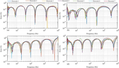
where |H(x,ω_j)|is the MATLAB simulation of Eq. (3) using the extracted parameters (R₀, R₁, C, and α), and y is the experimental magnitude response dataset. The MATLAB simulations using the extracted parameters show excellent agreement with the experimental results. As an example, the experimental Red Delicious electrode 1 data and MATLAB simulation of Eq. (3) using the extracted parameters are given in Fig. 6 as a solid line and gray circles, respectively. The errors between the MATLAB-simulated responses using the extracted parameters and the experimental data for each electrode pair are shown in Figs. 7a–7d for Granny Smith, Fuji, Red Delicious, and Spartan apples, respectively. The average error of each electrode pair is less than 0.3% for all apples, with maximum errors less than 3%; an exception is “electrode 2” for the Red Delicious apples, which has a maximum error of 7.5% at 1 MHz. These results suggest that the Cole impedance model provides an accurate representation of the apples’ impedance over this frequency range.

Figure 6. Comparison of experimental magnitude response (black) collected from Red Delicious electrode 1 configuration and MATLAB simulation using extracted parameters (gray circles).

Figure 7. Error using equivalent circuit parameters compared to experimental magnitude response from (a) Granny Smith, (b) Fuji, (c) Red Delicious, and (d) Spartan varieties of apples.

The ranges of values for each parameter in Table 1, that is, the difference between the maximum and minimum values, are as follows for the Granny Smith, Fuji, Red Delicious, and Spartan apples: (1) 150, 359, 363, and 170 Ω for R₀; (2) 2001, 5152, 5110 and 2774 Ω for R₁; (3) 6.08, 7.27, 4.4, and 4.02 nF for C; and (4) 0.0141, 0.0099, 0.0108, and 0.0039 for α. These ranges are all within the same order of magnitude for each apple and are expected to be a result of the electrode locations and not physiological changes occurring within the apple tissues, as less than 5 min was required to collect all seven sets of measurements for each apple. The following general trends are observed from the extracted parameters in Table 1: (1) both R₀ and R₁ increase in value with increasing distance between the measurement electrodes; (2) C decreases in value with increasing distance between the measurement electrodes; and (3) α shows the least change due to the location of the measurement electrodes.

Both R₀ and R₁ are typically maximum for the measurements collected between electrode 3, 4, or 5 and the reference electrode, whereas C is typically minimum for these measurements. These pairings have the greatest physical separation from the reference electrode and the most tissue between them, which could account for the increased resistance. To explore the parameter variability from multiple samples of each type of apple, the Cole impedance parameters were extracted from magnitude datasets of four additional apples of each type. This yielded a total of 35 extracted parameter sets for each variety of apple (7 measurements from each apple using the previously described electrode configurations), with a total of 140 parameter sets for this study. To visualize these full datasets, boxplots of all the extracted parameters are given in Figs. 8a–8d for R₀, R₁, C, and α, respectively. For this plot, the midline in each box represents the median value, and the top and bottom of each box are the 25th and 75th percentiles of the samples, respectively. The whiskers are drawn to the ends of the interquartile results, the outliers are shown as + symbols, and the notches display the variability of the median between samples. Box plots whose notches do not overlap have different medians at the 5% significance level.

Figure 8. Boxplots of extracted (a) R₀, (b) R₁, (c) C, (d) α for each electrode pair of all varieties of apples.

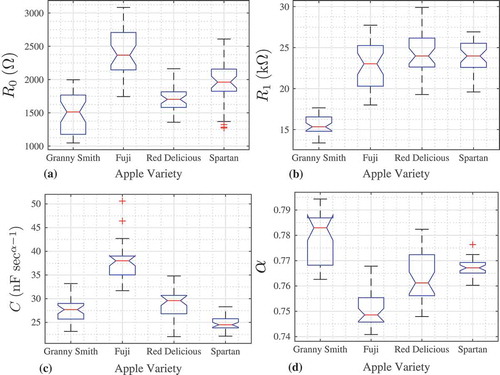
Figure 8 indicates that although the parameters for each type of apple fall within the same order of magnitude, there is a wide range of variability. The most extreme cases of this variability can be seen in Figs. 8c and 8d, where the range of values for the Spartan apples is significantly smaller than those for each of the other data types. The range of α for the Spartan measurements is 0.016, nearly half of the ranges of the other varieties (0.0318, 0.0270, and 0.0345 for Granny Smith, Fuji and Red Delicious, respectively). Therefore, the electrode position has a smaller impact on C and α for this type of apple compared to the other varieties, although further study is necessary to determine the cause of the different variabilities for each type of apple.

A comparison of the parameters extracted from all 20 apple samples illustrates that the previously identified trends for R₀, R₁, and C from the single apple parameters given in Table 1 are also present in this larger sample, with the largest resistances occurring for the electrode 3, 4, or 5 measurements in 15/20 and 20/20 sets of measurements for R₀ and R₁, respectively. The value of C is the lowest extracted from the data using these same electrode pairings in 14/20 sets of measurements. For a further comparison, the coefficient of variation (in %) for each parameter (R₀, R₁, C, and α) is presented in Table 2, calculated as

(6)

Table 2. Average and standard deviation of parameters from Granny Smith, Fuji, Red Delicious, and Spartan apples.

	R0 (Ω)			R1 (Ω)			C (nF s^α−1)			α
Apple	Avg.	SD	CV	Avg.	SD	CV	Avg.	SD	CV	Avg.	SD	CV
Granny Smith
1	1541	55.2	3.6	15.1k	646	4.27	25.9	1.88	7.26	0.784	4.2m	0.54
2	1826	109.8	6.01	16.3k	738	4.53	29.5	1.69	5.73	0.767	4.1m	0.53
3	1173	77.7	6.63	14.7k	799	5.46	25.9	1.24	4.79	0.787	0.8m	0.1
4	1757	69.5	3.96	14.4k	716	4.95	28.5	1.50	5.26	0.788	2.0m	0.25
5	1150	56.6	4.91	16.9k	859	5.1	28.2	1.56	5.53	0.769	2.1m	0.27
Fuji
1	2886	124.5	4.31	24.4k	2030	8.31	34.4	2.21	6.42	0.757	3.3m	0.44
2	2571	133.8	5.2	24.3k	920	3.78	39.8	1.60	4.12	0.746	3.5m	0.47
3	2149	46.0	2.14	25.7k	1653	6.44	35.2	2.03	5.77	0.757	6m	0.79
4	2005	117.8	5.87	19.5k	780	4.01	39.3	3.12	7.94	0.747	1.9m	0.25
5	2355	115.7	4.91	20.8k	1664	7.99	0.3	4.38	10.61	0.746	3m	0.4
Red Delicious
1	1961	127.5	6.5	27.4k	1723	6.29	23.9	1.38	5.77	0.776	3.6m	0.46
2	1568	79.2	5.05	24.8k	1298	5.23	31.2	1.49	4.78	0.752	2.4m	0.32
3	1793	71.8	4.00	25.2k	1277	5.07	27.6	1.09	3.95	0.771	2.7m	0.35
4	1543	87.1	5.64	21.3K	1076	5.05	31.2	1.62	5.19	0.761	1.3m	0.17
5	1678	59.4	3.54	22.9k	1385	6.05	30.6	1.83	5.98	0.757	1.6m	0.21
Spartan
1	1876	59.2	3.15	23.7k	975	4.12	25.6	1.37	5.35	0.769	1.4m	0.18
2	2074	95.8	4.62	24.7k	1092	4.41	25.6	1.34	5.23	0.764	1.6m	0.21
3	2035	80.5	3.95	24.1k	813	3.36	23.2	0.89	3.84	0.768	1.7m	0.22
4	2512	79.5	3.17	26.1k	503	1.93	24.3	0.94	3.87	0.765	2.1m	0.27
5	1346	50.0	3.71	21.3k	1048	4.92	24.7	0.85	3.44	0.77	3.4m	0.44

m = milli, the SI prefixes for 10⁻³; n = kilo, the SI prefixes for 10³.

where σ and µ are the mean and standard deviation, respectively, of the impedance parameters from each electrode extraction. These means and standard deviations are also given in Table 2 for reference. The coefficient of variation is used here to compare the variability of each parameter, as their widely different mean and standard deviations make a direct comparison difficult. Although the standard deviation for R₁ is the largest for each of the variables, the CV for R₀, R₁, and C are all within the same order of magnitude. That is, they show similar variations in the range of values based on the different electrode locations. Interestingly, α has the lowest CV, indicating that electrode location has the smallest impact on α when using this collection and extraction method.

Discussion

The magnitude responses in Fig. 5 and the extracted parameters in Table 1 illustrate that electrode location has a significant impact on the extracted impedance parameters using the two-electrode measurement setup with magnitude-only measurements. Parameters R₀, R₁, and C exhibit the most significant level of variation for all tested apple samples. The results presented in Ref.^[30] also support the notion that the variation in parameters is a result of only the electrode locations, where the selection of points for measurement has a significant impact on the impedance in three-dimensional fractional-order networks. However, further study is required to model an apple or other biological fruit as a 3D network of RC cells to compare the simulated impedance to experimental results before a final conclusion can be made as to whether electrode location is the most significant factor impacting the variations. The results of this study demonstrate that for situations in which the electrode location cannot be controlled, the change in impedance parameters should exceed the CV levels determined here to increase the confidence in the interpretation that these changes are truly an indicator of physiological change. Future studies should determine the variability of measurements collected with a four-electrode versus two-electrode arrangement, the variability of different measurement techniques (direct impedance, magnitude/phase only, time-domain), and the variability introduced by the extraction technique applied to identical datasets. This is important for determining the trade-offs between different measurement techniques and balancing the requirements for sample placement, precision circuitry, and signal processing that will be required to implement in a commercial method.

Another avenue for monitoring physiological changes with these parameters involves combinations of the parameters as opposed to using them individually. Combinations may exhibit lower variabilities if the parameters experience similar changes based on the electrode location, making them more suitable than R₀, R₁, C, or α independently. Two possibilities for monitoring the parameters are the ratio of resistor values (R₁/R₀) and the time constant (τ = (CR₁)^(1/α)), originally presented in Ref.^[19]. The mean, standard deviation, and CV for each of these combinations using the extracted impedance parameters for each electrode dataset are given in Table 3.

Table 3 Average, standard deviation, and coefficient of variation (%) of parameters from Granny Smith, Fuji, Red Delicious, and Spartan apples.

	R1/R0			τ = (CR1)^α (ms)
Apple	Avg.	SD	CV	Avg.	SD	CV
Granny Smith
1	9.83	0.31	3.15	45.30	1.42	3.13
2	8.94	0.27	3.02	46.98	0.96	2.04
3	12.51	0.54	4.32	44.57	0.918	2.06
4	8.24	0.34	4.13	50.7	0.542	1.07
5	14.66	0.17	1.16	47.38	1.384	2.92
Fuji
1	8.47	0.60	7.08	86.27	3.687	4.27
2	9.47	0.23	2.43	87.88	3.183	3.62
3	11.94	0.68	5.7	94.49	2.475	2.62
4	9.73	0.40	4.11	67.07	2.162	3.22
5	8.84	0.41	4.64	76.62	3.076	4.01
Red Delicious
1	13.98	0.49	3.51	79.17	1.136	1.43
2	15.87	1.09	6.87	72.53	2.586	3.57
3	14.05	0.28	1.99	79.57	1.329	1.67
4	13.82	0.58	4.20	66.03	0.996	1.51
5	13.64	0.75	5.50	67.63	1.055	1.56
Spartan
1	12.61	0.48	3.81	65.15	1.680	2.58
2	11.93	0.21	1.76	64.80	1.963	3.03
3	11.89	0.34	2.86	58.56	1.001	1.71
4	10.38	0.24	2.31	66.35	2.370	3.57
5	15.82	0.29	1.83	55.13	1.079	1.96

The ratio R₁/R₀ shows a slight improvement over the variabilities of the individual R₁ and R₀ values. However, the time constant, τ, shows the most improvement, suggesting that using a combination of the extracted parameters may be more suitable for monitoring than the individual values of other fruits and vegetables. This combination may be a better choice to assess the overall quality of a fruit, as each of the extracted circuit parameters could change as a result of different physiological processes, with the water content potentially impacting the resistance values and the cell membrane integrity impacting the capacitance. Therefore, τ could represent a better single figure of merit to investigate. The CV values in Tables 2 and 3 indicate the parameters or combinations least impacted by electrode position are α, τ, and R₁/R₀ (in that order). The parameter with the least variability based on the electrode location is the order, α, with relative changes of 0.5–1.8%. Therefore, α would make the best candidate to investigate for correlations to physiological changes in applications in which electrode location may be difficult to maintain for measurements taken over time. Although R₀, R₁, and C remain candidates for investigating correlations to physiological changes, their variabilities, which exceed 10%, necessitate further efforts to eliminate electrode position as their possible source of change.

Conclusion

This study demonstrated that the position of electrodes in a two-terminal electrode measurement system significantly impacts the values of equivalent circuit parameters extracted from magnitude-only measurements of apples. The parameters for all apples, in order from greatest to lowest variability, were C, R₁, R₀, and α. The first three parameters were shown to have variabilities in the range of 10–25%. α Showed little variation with regard to the electrode position, showing less than 1.8% variation for each of the apple varieties and thus making this parameter the most suitable candidate for future investigations into correlations between it and physiological changes experienced by apples under different conditions. Future research is still needed to determine whether these trends continue for other samples of this same variety of apple, samples of different varieties of apples, and samples of different varieties of fruit. Further research is also needed to determine whether these parameters can be monitored as an indicator of aging or ripening, physical damage, quality assessment, or any other type of assessment that is employed in the food processing industry.

References

- Ashtiani, S.H.; Salarikia, A.; Golzarian, M.; Emadi, B., Non-destructive Estimation of Mechanical and Chemical Properties of Persimmons by Ultrasonic Spectroscopy. International Journal of Food Properties 2015. 10.1080/10942912.2015.1126725
- Khodabakhshian, R.; et. al. Non-destructive Evaluation of Maturity and Quality Parameters of Pomegranate Fruit by Visible/Near Infrared Spectroscopy. International Journal of Food Properties 2016. 10.1080/10942912.2015.1126725
- Grimnesand, S.; Martinsen, O. Bioimpedance and Bioelectricity Basics; Academic Press, London, UK, 2000.
- El Khaled, D.; et. al. Cleaner Quality Control System Using Bioimpedance Methods: A Review for Fruits and Vegetables. Journal of Cleaner Production 2015. 10.1016/j.jclepro.2015.10.096
- Jackson, P.J.; Harker, F.R. Apple Bruise Detection by Electrical Impedance Measurement. Postharvest Biology & Technology 2000, 35, 104–107.
- Wu, L.; Ogawa, Y.; Tagawa, A. Electrical Impedance Spectroscopy Analysis of Eggplant Pulp and Effects of Drying and Freezing-thawing Treatments on Its Impedance Characteristics. Journal of Food Engineering 2007, 87, 274–280.
- Kuson, P.; Terdwongworakul, A. Minimally-destructive Evaluation of Durian Maturity Based on Electrical Impedance Measurement. Journal of Food Engineering 2012, 116, 50–56.
- Park, S.H.; Balasubramanian, V.M.; Sastry, S.K. Estimating Pressure Induced Changes in Vegetable Tissue Using In Situ Electrical Conductivity Measurement and Instrumental Analysis. Journal of Food Engineering 2013, 114, 47–56.
- Munoz-Huerta, R.F.;, et. al. An Analysis of Electrical Impedance Measurements Applied for Plant N Status Estimation in Lettuce (Lactuca sativa). Sensors 2014, 14, 11492–11503. 10.3390/s140711492
- Caravia, L.; Collins, C.; Tyerman, S.D. Electrical Impedance of Shiraz Berries Correlates with Decreasing Cell Vitality during Ripening. Australian Journal of Grape and Wine Research 2015, 21, 430–438.
- Zavadlav, S.; et. al. Assessment of Storage Shelf Life of European Squid (Cephalopod: Loliginidae, Loligo vulgaris) by Bioelectrical Impedance Measurements. Journal of Food Engineering 2016, 184, 44–52.
- Nakawajana, N.; Terdwongworakul, A.; Teerachaichayut, S. Minimally Destructive Assessment of Man- Gosteen Translucency Based on Electrical Impedance Measurements. Journal of Food Engineering 2016, 171, 137–144.
- Ando, Y.; Maeda, Y.; Mizutani, K.; Wakatsuki, N.; Hagiwara, S.; Nabetani, H. Effect of Air-dehydration Pretreatment before Freezing on the Electrical Impedance Characteristics and Texture of Carrots. Journal of Food Engineering 2016, 169, 114–121.
- Gonzalaz-Araiza, J.R.; Ortiz-Sanchez, M.C.; Vargas-Luna, M.; Cabrera-Sixto, J.M. Application of Electrical Bio-impedance Evaluation of Strawberry Ripeness. International Journal of Food Properties 2016. 10.1080/10942912.2016.1199033
- Freeborn, T.J. A Survey of Fractional-order Circuit Models for Biology and Biomedicine. IEEE Journal on Emerging and Selected Topics Circuits and Systems 2013, 3, 416–424.
- Podlubny, I. Fractional Differential Equations; Academic Press, London, UK, 1999.
- Ortigueira, M.D. Fractional Calculus for Scientists and Engineers; Springer, London, UK, 2011.
- Galvao, R.K.H. et. al. Fractional Order Modeling of Large Three-dimensional RC Networks. IEEE Transactions on Circuits and Systems I 2013, 60, 624–637.
- Jacyntho, L.A. et. al. Identification of Fractional-order Transfer Functions Using a Step Excitation. IEEE Transactions on Circuits and Systems II 2015, 62, 896–900.
- Elwakil, A.S.; Maundy, B. Extracting the Cole-Cole Impedance Model Parameters without Direct Impedance Measurement. Electronics Letters 2010, 46, 1367–1368.
- Maundy, B.J.; Elwakil, A.S.; Allagui, A. Extracting the Parameters of the Single-Dispersion Cole Bioimpedance Model Using a Magnitude-only Method. Computers and Electronics in Agriculture 2015, 119, 153–157.
- Freeborn, T.J.; Maundy, B.; Elwakil, A.S. Cole Impedance Extractions from the Step-response of a Current Excited Fruit Sample. Computers and Electronics in Agriculture 2013, 98, 100–108.
- Maundy, B.; Elwakil, A.S. Extracting Single Dispersion Cole-Cole Impedance Model Parameters Using an Integrator Setup. Analog Integrated Circuits and Signal Processing 2012, 71, 107–110.
- Freeborn, T.J.; Maundy, B.; Elwakil, A.S. Improved Cole-Cole Parameter Extraction from Frequency Response Using Least Squares Fitting. IEEE International Symposium on Circuits & Systems. 2012, 337–340.
- Fang, Q.; Liu, X.; Cosic, I. Bioimpedance Study on Four Apple Varieties. 13th International Conference on Electrical Bioimpedance & 8th Conference on Electrical Impedance Tomography. 2007, 114–117. doi: 10.1007/978-3-540-73841-1_132
- Yuxiang, Y.; Wenwen, N.; Sun, Q.; Wen, H.; Teng, Z. Improved Cole Parameter Extraction Based on the Least Absolute Deviation Method. Physiological Measurements 2013, 34, 1239–1252.
- Gholami-Boroujeny, S.; Bolic, M., Extraction of Cole Parameters from the Electrical Bioimpedance Spectrum Using Stochastic Optimization Algorithms. Medical & Biological Engineering & Computing 2016, 54, 643–651. 10.1007/s11517-015-1355-y
- Freeborn, T.J.; Maundy, B.; Elwakil, A.S., Extracting the Parameters of the Double-Dispersion Cole Bioimpedance Model from Magnitude Response Measurements. Medical & Biological Engineering & Computing 2014, 52, 749–758. 10.1007/s11517-014-1175-5
- Freeborn, T.J.; Maundy, B.; Elwakil, A.S. Factors Impacting Accurate Cole-impedance Extractions from Magnitude-only Measurements. IEEE Conference on Systems, Man, and Cybernetics. 2016, 223–227.
- Zhou, K.; et. al. Fractional-Order Three-dimensional ∆ × N Circuit Network. IEEE Transactions on Circuits and Systems I 2015, 62, 2401–2410.