A shape equation for Hayward Kiwifruit

ABSTRACT

In this paper, a new shape equation for Hayward kiwifruit is developed. Being simple and generic, it required only the major measurable dimensions of a kiwifruit as inputs (length, major-diameter, and minor-diameter). The equation was validated against empirical shape data with a maximum 3.09% error. The new shape equation can estimate important metrics, such as volume, mass and surface area. Equation development was generalized, so shape equations for other crops could be produced using the same methodology. The simplicity and speed of this new method allow realistic populations of Hayward kiwifruit to be rapidly generated in a modeling environment.

KEYWORDS:

• Shape description
• model generation
• biological variability
• CAD models
• kiwifruit

Introduction

Mathematical modeling is being increasingly utilized to innovate and optimize key pre- and post-harvest processes, vital to the success of the horticultural cold-chain.^[1–5] One current challenge in the model development process for products of biological origin is the definition and construction of an accurate 3D model geometry. Fruits and vegetables are in particular produced with a wide variability in shape and size, even within a given cultivar. Environmental, nutritional and production management differences result in each fruit having a unique size, mass, and shape.^[6–9] Taking this natural variability into account is a key obstacle to engineering efficient processes in the horticultural industry, with larger design tolerances being required to operate competently compared with other industries, driving up costs.^[10] Commercially, variances in size and shape are typically managed in the sorting and packing processes, where morphological defects are removed and produce is electronically sorted into mass ranges.^[11–13] Even so, within a size range, there still remains a range of size and shape.

In this paper, a new shape equation for Hayward kiwifruit is developed, to create a process for rapidly generating populations of fruit shapes and sizes in a computational environment. Kiwifruit was chosen as the subject of this study because it is the largest fresh horticultural export of the authors’ home nation, New Zealand.^[14] The primary requirements to this new approach is that: (1.) it can be conducted independent of shape input data (such as^[15,16] and^[3]); (2.) it performs better than ellipsoid approximation; (3.) it is sufficiently simple to implement as a few short lines of code, in order to execute natively in modelling software such as COMSOL or Blender, and; (4.) it can be used to draw an accurate 3D kiwifruit of any size or shape with little to no modification of the original equation(s). The best method to meet these criteria is an algebraic function that follows the longitudinal profiles of a Hayward kiwifruit, and can be scaled/sized to different grades by setting the value of several scale factors – ideally, the measurable dimensions of a kiwifruit.

Methodology

Development of a shape equation for Hayward kiwifruit

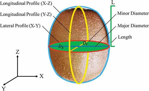
The major geometrical attributes of a single ‘Hayward’ kiwifruit (Actinidia deliciosa) are: length (distance from the largest axial cross section to the apex),$L$; major axis (maximum distance at the largest axial cross section), $D_X$; and minor axis (minimum distance at the largest axial cross-section, perpendicular to the major axis), $D_Y$ (Figure 1). The shape of a kiwifruit has three profiles: the lateral X-Y profile (red line), a function of $D_X$ and $D_Y$; the longitudinal X-Z profile (blue line), a function of $D_X$ and $L$; and the longitudinal Y-Z profile (yellow line), a function of $D_Y$ and $L$ (Figure 1). In this section algebraic functions are developed that represent the lateral and longitudinal profiles of a ‘Hayward’ kiwifruit.

Figure 1. A generic ‘Hayward’ kiwifruit with the major geometrical attributes highlighted: $D_X$ = major axis; $D_Y$ = minor axis; $L$ = length

An anonymous industrial partner provided shape data of count 36 ‘Hayward’ kiwifruit to help develop and validate a shape equation (Figure 2).^[11] The information was empirically determined lateral and longitudinal profiles, derived by sketching the outlines of 117 fruit, producing maximum, minimum and average fruit size within the count 36 mass range. As this information is commercially sensitive, Figure 2 is not to scale and the scale has been omitted. Subsequent analysis and discussion of kiwifruit shape and size use dimensionless lengths.

Figure 2. Empirical shape profiles in the (a) X-Z, (b) Y-Z, and (c) X-Y directions for count 36 Hayward kiwifruit. Minimum (min), average (av) and maximum (max) profiles are the result of tracing the shape of 117 fruit.^[11] Images not to scale; scale omitted to preserve data confidentiality

Although the entire volume of the kiwifruit cannot be described as an ellipsoid,^[17] the lateral profile (Figure 2c) is nearly elliptical. Ellipses with the same major and minor axes as $D_X$ and $D_Y$ are compared to the empirical lateral profiles in Figure 2c. The differences in area were minimal, with an error of 0.26%, 0.39% and 1.61% for the minimum, average and maximum lateral profiles, respectively. These low errors demonstrate an ellipse can accurately describe the lateral profile of a Hayward kiwifruit.

Kiwifruit do not have an elliptical longitudinal profile.^[17] Instead, kiwifruit are relatively flat near the center of the fruit, and then curve sharply at the apices to form a shoulder (see Figure 2a and b), a shape distinct from an ellipse. An algebraic function was developed that has this behavior, named a longitudinal profile function (LPF). The general form of an LPF is:

(1) $d_{j,k}=f_1\left(D_j,L_k,Z\right)$(1)

where $f_1$ is the LPF, a function of the diameter of the fruit ($D$), the length of the fruit ($L$) and the distance from the center of the fruit (largest axial cross-section) to the apices ($Z$). As there are two longitudinal profiles, there are two LPFs – one each for the X-Z and Y-Z directions; indicated by subscript $j$, where $j=X$ or $Y$. The origin of the Z-axis (where $Z=0$) is the largest axial cross-section, marked as the X-centre and Y-centre on Figure 2. Separate LPFs can be considered for the top (calyx) and bottom (stem) halves of the fruit. This is indicated by subscript $k$, where $k=calyx$ or $stem$. The LPF ($f_1$) gives $d$, the distance from the Z-centre line to the outer edge of the fruit along the X- or Y-axis, at any point along the Z-axis. It is assumed there is symmetry along the Z-centre line. This is a valid assumption as the fruit is graded to eliminate significant morphological deformities prior to packaging.^[11]

At the center of the fruit ($Z=0$), the output of the function must be $d_X=D_X$ or $d_Y=D_Y$; and at the apex of the fruit ($Z=L_k$), the output must be zero, $d_j=0$. Within the limits of 0 $\le$ $Z$ $\le$ $L_k$, this behavior is given by:

(2) $f_1=\frac{L_k-f_2\left(L_k,Z\right)}{L_k}\times D_j$(2)

where $f_2$ defines the rate that $d$ changes with respect to $Z$. $f_2$ also has limits where at $Z$ = 0,

$f_2$ = 0; and at $Z$ = $L_k$, $f_2$ = $L_k$. $f_2$, therefore, influences the rate at which $d$ diminishes to 0: if there is a linear relationship between $d$ and $Z$, the profile is a straight line:

(3) $f_2=Z$(3)

For an elliptical profile:

(4) $f_2=L_k-\sqrt{{L_k}^2-Z^2}$(4)

So that the LPF for an ellipsoid is:

(5) $d_{j,k}=\frac{\sqrt{{L_k}^2-Z^2}}{L_k}\times D_j$(5)

As a kiwifruit is relatively flat in the middle and forms a sharp shoulder near the stem or calyx, $f_2$ needs to be a function that diminishes slowly at low to medium values of $Z$, and then quickly diminishes to 0 as $Z$ approaches $L_k$. This is achieved by using an exponential function:

(6) $f_2=exp\left(Z\right)-1$(6)

However, Equation (6)(6) $f_2=exp\left(Z\right)-1$(6) violates the limits imposed for $f_2$ (when $Z$ = 0, $f_2$ = 0 and when $Z$ = $L_k$, $f_2$ = $L_k$), so the following additions are required:

(7) $f_2=\frac{L_k}{exp\left(S\right)-1}\times \left(exp\left(\frac{S\times Z}{L_k}\right)-1\right)$(7)

where $S$ is added as a ‘shoulder coefficient’, where different values of $S$ impact the steepness or flatness of the curve. Substituting Equation (7)(7) $f_2=\frac{L_k}{exp\left(S\right)-1}\times \left(exp\left(\frac{S\times Z}{L_k}\right)-1\right)$(7) into Equation (2)(2) $f_1=\frac{L_k-f_2\left(L_k,Z\right)}{L_k}\times D_j$(2) gives the LPF for kiwifruit:

(8) $d_{j,k}=\frac{L_k-\left(\frac{L_k}{exp\left(S\right)-1}\times \left(exp\left(\frac{S\times Z}{L_k}\right)-1\right)\right)}{L_k}\times D_j$(8)

Non-linear least squared regression (MATLABs ‘lsqnonlin’ function) was used to determine the $S$ that minimizes the difference between the new LPF and the average empirical profile provided by^[11] in each of the four scenarios. Performance is assessed in Figure 3. Equation (6)(6) $f_2=exp\left(Z\right)-1$(6) showed a much closer agreement to the average empirical profiles than an ellipse: while the ellipse routinely under predicted the true shape of a kiwifruit, the new LPF was within the bounds of variability in three out of four comparisons.

Figure 3. Comparison of Longitudinal Profile Functions (LPFs) with empirical shape data for Hayward kiwifruit: Red = empirical shape data; blue = new LPF (Equation 6(6) $f_2=exp\left(Z\right)-1$(6) ); and cyan = an ellipsoid

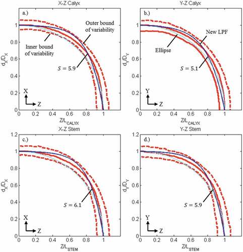
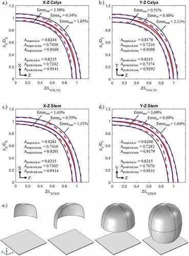
Although the new LPF shows a closer agreement to the average empirical profile, there was still an over prediction near the middle of the fruit and an underprediction near the apices. The level of error was problematic, as ideally the shape equation for kiwifruit should be able to produce an accurate fruit shape of any size within the given range, not just an ‘average’ sized fruit. As shown in Figure 3, an ellipse lacks the relative flatness near the middle of the fruit, but has a softer curve near the apices; and conversely, the new LPF curves too sharply toward the apices, but is flatter near the middle. Therefore, the two profiles are complementary and can be combined to help mitigate the deficiencies of the other. This gives an updated LPF for kiwifruit:

(9) $d_{j,k}=\left(\left[\frac{L_k-\left(\frac{L_k}{exp\left(S\right)-1}\times \left(exp\left(\frac{S\times Z}{L_k}\right)-1\right)\right)}{2\cdot L_k}\right]+\left[\frac{\sqrt{{L_k}^2-Z^2}}{2\cdot L_k}\right]\right)\times D_j$(9)

The performance of Equation (9)(9) $d_{j,k}=\left(\left[\frac{L_k-\left(\frac{L_k}{exp\left(S\right)-1}\times \left(exp\left(\frac{S\times Z}{L_k}\right)-1\right)\right)}{2\cdot L_k}\right]+\left[\frac{\sqrt{{L_k}^2-Z^2}}{2\cdot L_k}\right]\right)\times D_j$(9) is explored in Figure 4. The shoulder coefficient $S$ = 7.0 was found by minimizing the mean percentage error across all comparisons (12 comparisons in total: the minimum, maximum and average profiles for the Z-X, Z-Y, stem and calyx directions). Equation (9)(9) $d_{j,k}=\left(\left[\frac{L_k-\left(\frac{L_k}{exp\left(S\right)-1}\times \left(exp\left(\frac{S\times Z}{L_k}\right)-1\right)\right)}{2\cdot L_k}\right]+\left[\frac{\sqrt{{L_k}^2-Z^2}}{2\cdot L_k}\right]\right)\times D_j$(9) performs well at predicting the average kiwifruit longitudinal profile (maximum error of 0.55%) and also accurate across the 12 comparisons, with a maximum error of just 3.09% in the case of the minimum Y-Z stem profile (Figure 4d).

Figure 4. (a–d) Dimensionless empirical minimum, average and maximum shape profiles for count 36 Hayward kiwifruit (red) compared with the updated LPF (Equation 9(9) $d_{j,k}=\left(\left[\frac{L_k-\left(\frac{L_k}{exp\left(S\right)-1}\times \left(exp\left(\frac{S\times Z}{L_k}\right)-1\right)\right)}{2\cdot L_k}\right]+\left[\frac{\sqrt{{L_k}^2-Z^2}}{2\cdot L_k}\right]\right)\times D_j$(9) ) where $S$= 7.0 (blue; Equation (9)(9) $d_{j,k}=\left(\left[\frac{L_k-\left(\frac{L_k}{exp\left(S\right)-1}\times \left(exp\left(\frac{S\times Z}{L_k}\right)-1\right)\right)}{2\cdot L_k}\right]+\left[\frac{\sqrt{{L_k}^2-Z^2}}{2\cdot L_k}\right]\right)\times D_j$(9) ); (e) Creating a kiwifruit in COMSOL as eight parametric surfaces

Equation (9)(9) $d_{j,k}=\left(\left[\frac{L_k-\left(\frac{L_k}{exp\left(S\right)-1}\times \left(exp\left(\frac{S\times Z}{L_k}\right)-1\right)\right)}{2\cdot L_k}\right]+\left[\frac{\sqrt{{L_k}^2-Z^2}}{2\cdot L_k}\right]\right)\times D_j$(9) therefore represents a single equation that requires only three input parameters, the measurable major geometric attributes of a kiwifruit ($D_X$, $D_Y$ and $L$) and one constant ($S$ = 7.0) that can accurately describe both the X-Z and Y-Z longitudinal profiles for any fruit size within the count 36 mass range.

Application of shape equation

Implementation in CAD and modeling software

Equation (9)(9) $d_{j,k}=\left(\left[\frac{L_k-\left(\frac{L_k}{exp\left(S\right)-1}\times \left(exp\left(\frac{S\times Z}{L_k}\right)-1\right)\right)}{2\cdot L_k}\right]+\left[\frac{\sqrt{{L_k}^2-Z^2}}{2\cdot L_k}\right]\right)\times D_j$(9) can be implemented natively into modeling software such as COMSOL^[18] or Blender^[19] to draw 3D kiwifruit shapes through the use of a parametric surface. Parametric surfaces are generally described by:

(10) $r\left(u,v\right)=f_X\left(u,v\right)+f_Y\left(u,v\right)+f_Z\left(u,v\right)$(10)

where the three functions $f_X$, $f_Y$ and $f_Z$ each specify the shape of the surface in the x, y and z dimensions, respectively. The $u$ variable is the radial coordinate direction, so that 0 $\le$ $u$ $\le$ 2$\pi$; and $v$ is the coordinate in the vertical direction, so that $f_Z$ = $v$ and 0 $\le$ $v$ $\le$ $L_k$. $f_X$ and $f_Y$ are the LPF for kiwifruit (Equation 9(9) $d_{j,k}=\left(\left[\frac{L_k-\left(\frac{L_k}{exp\left(S\right)-1}\times \left(exp\left(\frac{S\times Z}{L_k}\right)-1\right)\right)}{2\cdot L_k}\right]+\left[\frac{\sqrt{{L_k}^2-Z^2}}{2\cdot L_k}\right]\right)\times D_j$(9) ) in the x and y directions, respectively, – but $D_X$ and $D_Y$ are replaced with $D_X\cdot \mathrm{c}\mathrm{o}\mathrm{s}\left(u\right)$ and $D_Y\cdot \mathrm{s}\mathrm{i}\mathrm{n}\left(u\right)$, respectively, to transform into the radial coordinate direction, $u$. $Z$ is simply transformed to be equal to $v$ as these coordinate directions are both equivalent (for more details on surfaces, see^[20]). These transformations give:

(11) $\begin{array}{rl}& r\left(u,v\right)=\left(\left[\frac{L_k-\left(\frac{L_k}{exp\left(S\right)-1}\times \left(exp\left(S\cdot v/L_k\right)-1\right)\right)}{2\cdot L_k}\right]+\left[\frac{\sqrt{{L_k}^2-v^2}}{2\cdot L_k}\right]\right)\\ & \times D_X\cdot cos\left(u\right)+\\ & \left(\left[\frac{L_k-\left(\frac{L_k}{exp\left(S\right)-1}\times \left(exp\left(S\cdot v/L_k\right)-1\right)\right)}{2\cdot L_k}\right]+\left[\frac{\sqrt{{L_k}^2-v^2}}{2\cdot L_k}\right]\right)\\ & \times D_Y\cdot sin\left(u\right)+v\end{array}$(11)

Using the shape equation in modeling software such as COMSOL is summarised in Figure 4e. Digital kiwifruit analogs were divided into eight faces, similar to how COMSOL creates spheres and ellipses. Therefore, eight separate parametric surfaces were created to describe the kiwifruit. In Blender, kiwifruits were created in a similar fashion using the ‘XYZ Math Surface’ function.

Volume and surface area

Given that the cross-section of a Hayward kiwifruit can be modeled as an ellipse, a kiwifruit can be modeled as a stack of elliptical disks. Therefore, Equation (9)(9) $d_{j,k}=\left(\left[\frac{L_k-\left(\frac{L_k}{exp\left(S\right)-1}\times \left(exp\left(\frac{S\times Z}{L_k}\right)-1\right)\right)}{2\cdot L_k}\right]+\left[\frac{\sqrt{{L_k}^2-Z^2}}{2\cdot L_k}\right]\right)\times D_j$(9) can be used to determine the size of each disk in the stack, and the volume and surface area^[21] of a kiwifruit of a given size (set of $D_X$, $D_Y$ and $L$ values) can be numerically determined, using the disk method.^[22]

With reference to Figure 5a, the first elliptical disk at the center of the fruit has the same major and minor diameters as $D_X$ and $D_Y$. The size of subsequent disks along the Z-axis is determined from Equation (9)(9) $d_{j,k}=\left(\left[\frac{L_k-\left(\frac{L_k}{exp\left(S\right)-1}\times \left(exp\left(\frac{S\times Z}{L_k}\right)-1\right)\right)}{2\cdot L_k}\right]+\left[\frac{\sqrt{{L_k}^2-Z^2}}{2\cdot L_k}\right]\right)\times D_j$(9) , where the thickness of each disk is dependent on the number of disks used:

(12) $\mathrm{\Delta }Z=\frac{L_k}{I}$(12)

Figure 5. Numerical calculation of (a) volume and (b) surface area using the disk technique (Riddle, 1974)

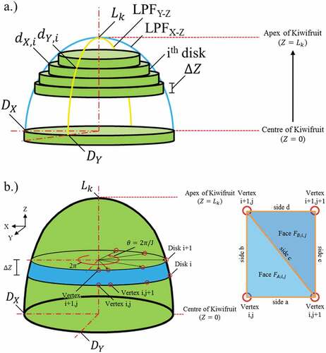
where $I$ is the total number of elliptical disks and $\mathrm{\Delta }Z$ is the thickness of each disk. The volume disk $i$ out of a total number of disks $I$ is:

(13) $V_i=\pi \cdot d_{X,i}\cdot d_{Y,i}\cdot \mathrm{\Delta }Z$(13)

So that the volume of a kiwifruit can be estimated numerically as the sum of all disks:

(14) $V=2\sum _{i=1}^I\pi \cdot d_{X,i}\cdot d_{Y,i}\cdot \mathrm{\Delta }Z$(14)

where Equation (14)(14) $V=2\sum _{i=1}^I\pi \cdot d_{X,i}\cdot d_{Y,i}\cdot \mathrm{\Delta }Z$(14) assumes $L_{calyx}$ = $L_{stem}$.

A similar numerical approach is used for the determination of surface area. With reference to Figure 5b, elliptical disks are discretized in the radial direction to form $J$ number of vertexes, the angle between each vertex being 2$\pi /J$ radians. This is used to calculate the x, y, and z coordinates of each vertex:

(15) ${\theta }_j=j\cdot \frac{2\pi }{J}$(15)

(16) ${\mathbb{V}}_{X,i,j}=sin\left({\theta }_j\right)\cdot \sqrt{\frac{1}{{\left(\frac{sin\left({\theta }_j\right)}{d_{X,i}}\right)}^2+{\left(\frac{cos\left({\theta }_j\right)}{d_{Y,i}}\right)}^2}}$(16)

(17) ${\mathbb{V}}_{Y,i,j}=cos\left({\theta }_j\right)\cdot \sqrt{\frac{1}{{\left(\frac{sin\left({\theta }_j\right)}{d_{X,i}}\right)}^2+{\left(\frac{cos\left({\theta }_j\right)}{d_{Y,i}}\right)}^2}}$(17)

(18) ${\mathbb{V}}_{Z,i,j}=Z_i$(18)

where $\mathbb{V}$ is a single vertex. Vertexes${\mathbb{V}}_{i,j}$, ${\mathbb{V}}_{i,j+1}$, and ${\mathbb{V}}_{i+1,j}$ form a triangular face $F_{A,i,j}$ and vertexes ${\mathbb{V}}_{i,j+1}$, ${\mathbb{V}}_{i+1,j}$, and ${\mathbb{V}}_{i+1,j+1}$ form triangular face $F_{B,i,j}$. The area of the two faces are determined using Heron’s formula^[23] by calculating the lengths of the sides of each triangle:

(19) $a=\overline{{\mathbb{V}}_{i,j}{\mathbb{V}}_{i,j+1}}$(19)

(20) $b=\overline{{\mathbb{V}}_{i,j}{\mathbb{V}}_{i+1,j}}$(20)

(21) $c=\overline{{\mathbb{V}}_{i+1,j}{\mathbb{V}}_{i,j+1}}$(21)

(22) $d=\overline{{\mathbb{V}}_{i+1,j}{\mathbb{V}}_{i+1,j+1}}$(22)

(23) $e=\overline{{\mathbb{V}}_{i,j+1}{\mathbb{V}}_{i+1,j+1}}$(23)

(24) $F_{A,i,j}=\frac{1}{4}\sqrt{\left(a+b+c\right)\left(-a+b+c\right)\left(a-b+c\right)\left(a+b-c\right)}$(24)

(25) $F_{B,i,j}=\frac{1}{4}\sqrt{\left(c+d+e\right)\left(-c+d+e\right)\left(c-d+e\right)\left(c+d-e\right)}$(25)

The surface area can, therefore, be determined numerically by summing the area of all triangular faces:

(26) $A=\sum _{i=1}^{I-1}\sum _{j=1}^{J-1}{F}_{A,i,j}+F_{B,i,j}$(26)

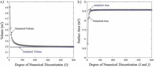
The accuracy of these numerical methods is dependent on the level of discretization ($I$ and $J$ values). This is explored by coding the above numerical methods into a MATLAB script and applying them to a sphere with a radius of 1 m at various levels of discretization. Results are shown in Figure 6, where the volume and surface area approaches the analytical solution at relatively low levels of discretization.

Figure 6. Efficacy of using the disk method to numerically approximate the (a) volume and (b) surface area of a sphere (radius = 1 m) as a function of the degree of numerical discretization resolution

Results and discussion

Validation

Figure 4 serves as a validation of the shape equation for kiwifruit (Equation 9(9) $d_{j,k}=\left(\left[\frac{L_k-\left(\frac{L_k}{exp\left(S\right)-1}\times \left(exp\left(\frac{S\times Z}{L_k}\right)-1\right)\right)}{2\cdot L_k}\right]+\left[\frac{\sqrt{{L_k}^2-Z^2}}{2\cdot L_k}\right]\right)\times D_j$(9) ) within the count 36 size range, however, a further validation was performed for fruit outside of this range.^[16] measured the major diameter ($D_X$), minor diameter ($D_Y$) and length ($L$) of 15 Hayward kiwifruit ranging from 55.3 to 112.3 g, and then measured the volume of each fruit using the water displacement method. These values of $D_X$, $D_Y$, and $L$ where used to predict fruit volume using the shape equation for kiwifruit (Equation 9(9) $d_{j,k}=\left(\left[\frac{L_k-\left(\frac{L_k}{exp\left(S\right)-1}\times \left(exp\left(\frac{S\times Z}{L_k}\right)-1\right)\right)}{2\cdot L_k}\right]+\left[\frac{\sqrt{{L_k}^2-Z^2}}{2\cdot L_k}\right]\right)\times D_j$(9) ) and the disk method ($I$ = 500), which was then compared to the measured values. Ellipsoids (Equation 5(5) $d_{j,k}=\frac{\sqrt{{L_k}^2-Z^2}}{L_k}\times D_j$(5) ) with the same semi-axis dimensions as the fruit were also compared. Results are shown in Figure 7a. Ellipsoids routinely under predicted the true volume by a significant margin, and had a mean error of 8.5%. The new shape equation performed much better, neither consistently over nor under predicting the true volume, and had a mean error of just 2.5%.

Figure 7. Comparison of predicted volumes using the new shape equation for kiwifruit (crosses; Equation 9)(9) $d_{j,k}=\left(\left[\frac{L_k-\left(\frac{L_k}{exp\left(S\right)-1}\times \left(exp\left(\frac{S\times Z}{L_k}\right)-1\right)\right)}{2\cdot L_k}\right]+\left[\frac{\sqrt{{L_k}^2-Z^2}}{2\cdot L_k}\right]\right)\times D_j$(9) and ellipsoids (circles; Equation 5)(5) $d_{j,k}=\frac{\sqrt{{L_k}^2-Z^2}}{L_k}\times D_j$(5) with measured volumes (dashed line) of kiwifruit ranging from 55.3 to 112.3 g.^[16]

Developing shape equations for other fruit

The process described above has potential to be generalized, so that shape equations for other fruits can be created. Generating new shape equations requires careful consideration of the nature of the $f_2$ function (Equation 2(2) $f_1=\frac{L_k-f_2\left(L_k,Z\right)}{L_k}\times D_j$(2) ), which defines the rate at which $d$ approaches zero as the length $Z$ approaches the apex, $L_k$. It is also likely that most fruit items consist of multiple LPFs, and cannot be considered symmetrical along one or more planes. For example, a pear could be simplified to be symmetrical along the X-Z and Y-Z planes (in relation to directions displayed in Figure 1), but not along the X-Y plane. The LPF for the bottom half of a pear could be an ellipsoid ($L_{calyx}\le Z\le 0$; Equation 5(5) $d_{j,k}=\frac{\sqrt{{L_k}^2-Z^2}}{L_k}\times D_j$(5) ), but a new LPF would be required for the top half of the pear. This LPF would need to incorporate a step change in the decline of $d$ at different values of $Z$, where $d$ declines rapidly at low values of $Z$ but then does not decline at all at medium values of $Z$, forming the ‘neck’ of the pear. As $Z$ approaches $L_{stem}$, $d$ should again start to decline, to be equal to zero at the top of the fruit.

Alternatively, an LPF can be derived from empirical shape data through the use of a Fourier series, similar to^[15]:

(27) $R_{j,k}=a_0+\sum _{n=1}^N{a}_{n}cos\left(n\theta \right)+\sum _{n=1}^N{b}_{n}sin\left(n\theta \right)$(27)

Equation (27)(27) $R_{j,k}=a_0+\sum _{n=1}^N{a}_{n}cos\left(n\theta \right)+\sum _{n=1}^N{b}_{n}sin\left(n\theta \right)$(27) uses polar coordinates, so relating it back to the LPF format requires $d$ = $\sqrt{R^2-Z^2}$ and $Z$ = $R\cdot \mathrm{c}\mathrm{o}\mathrm{s}\left(\theta \right)$, where $\theta$ = 0$\to$0.5$\pi$. This approach requires empirical data to function, so a data library of fruit shapes must be acquired first, but the acquisition of the harmonics can be automated, making it a universal approach. For example, the LPF developed for a kiwifruit (Equation 9(9) $d_{j,k}=\left(\left[\frac{L_k-\left(\frac{L_k}{exp\left(S\right)-1}\times \left(exp\left(\frac{S\times Z}{L_k}\right)-1\right)\right)}{2\cdot L_k}\right]+\left[\frac{\sqrt{{L_k}^2-Z^2}}{2\cdot L_k}\right]\right)\times D_j$(9) ), expressed as a Fourier series with 10 harmonics was $a_0$ = 1.017, $a_n$ = [−0.00398, 0.000657, −0.00984, −0.00915, −0.000949, 0.00164, 0.00241, 0.00120, 7.32E-5, −0.000163] and $b_n$ = [0.00405, 0.00658, 0.00630, −0.00504, −0.00624, −0.00350, −0.00116, 0.000549, 0.000422, 6.55E-5] for $L_k$ = 1 and $D_{j,k}$ = 1. While more flexible in some senses, Equation (27)(27) $R_{j,k}=a_0+\sum _{n=1}^N{a}_{n}cos\left(n\theta \right)+\sum _{n=1}^N{b}_{n}sin\left(n\theta \right)$(27) is more difficult to implement natively in modeling software, and new harmonics would need to be derived with any changes to $L_k$ or $D_j$.

Conclusion

A new shape equation for Hayward kiwifruit was developed. By developing a Longitudinal Profile Function and combining it with a parametric surface, accurate 3D kiwifruit shapes of any size can be created using only a single equation. This equation can be combined with the disk method to quickly estimate volume, mass and surface area for a given set of major dimensions, namely the fruit length, major diameter, and minor diameter. The new equation showed a very close agreement to empirical data, when compared in terms of shape and volume across a wide range of fruit sizes. The new equation can be implemented trivially into modeling software such as COMSOL or Blender, enabling the modeling and potential optimization of key kiwifruit pre- and post-harvest operations. There is potential for this approach to be generalized by developing new LPFs for other crops.

Nomenclature

$a_0$:	=	scaling factor of Fourier series
$a_n$, $b_n$:	=	harmonics of Fourier series
$A$:	=	area (m2)
$a$, $b$, $c$, $d$, $e$:	=	length of a side of triangle (m)
$D$:	=	fruit diameter (m)
$d$:	=	distance (m)
$F$:	=	area of triangle (m2)
$f$:	=	function
$I$:	=	number of discretizations, vertical direction
$J$:	=	number of discretisations, radial direction
$L$:	=	fruit length (m)
$R$:	=	radius (m)
$r$:	=	parametric surface
$S$:	=	shoulder coefficient
$u$:	=	coordinates in radial direction
$V$:	=	volume (m3)
$v$:	=	coordinates in vertical direction
$X$, $Y$, $Z$:	=	direction in Cartesian coordinates

Greek symbols

$\theta$:

=

angle, radians

Miscellaneous symbols

$\mathbb{V}$:

=

vertex

Subscripts

$A$, $B$:	=	triangle
$j$:	=	direction, X or Y
$k$:	=	apex of kiwifruit, calyx or stem
$X$, $Y$, $Z$:	=	direction in Cartesian coordinates

Acknowledgments

The authors gratefully acknowledge the New Zealand Ministry of Business, Innovation and Employment for funding this work (Fibreboard Packaging Design Project, MAUX1302). We also appreciate the help of students Angela Yang and Julia Zhou for their assistance.

Additional information

Funding

This work was supported by the Ministry of Business, Innovation and Employment [MAUX1302].

References

- Defraeye, T.; Lambrecht, R.; Delele, M. A.; Tsige, A. A.; Opara, U. L.; Cronjé, P.; Verboven, P.; Nicolai, B. Forced-Convective Cooling of Citrus Fruit: Cooling Conditions and Energy Consumption in Relation to Package Design. J. Food Eng. 2014, 121, 118–127. DOI: 10.1016/j.jfoodeng.2013.08.021.
- Ferrua, M. J.; Singh, R. P. Modeling the Forced-Air Cooling Process of Fresh Strawberry Packages, Part I: Numerical Model. Int. J. Refrig. 2009, 32(2), 335–348. DOI: 10.1016/j.ijrefrig.2008.04.010.
- O’Sullivan, J.; Ferrua, M. J.; Love, R.; Verboven, P.; Nicolaï, B.; East, A. R. Modelling the Forced-Air Cooling Mechanisms and Performance of Polylined Horticultural Produce. Postharvest. Biol. Technol. 2016, 120, 23–35. DOI: 10.1016/j.postharvbio.2016.05.008.
- Stopa, R.; Komarnicki, P.; Szyjewicz, D.; Kuta, Ł. Modeling of Carrot Root Radial Press Process for Different Shapes of Loading Elements Using the Finite Element Method. Int. J. Food Prop. 2017, 20(sup1), S340–S352. DOI: 10.1080/10942912.2017.1296862.
- Stopa, R.; Szyjewicz, D.; Komarnicki, P.; Kuta, Ł. Limit Values of Impact Energy Determined from Contours and Surface Pressure Distribution of Apples under Impact Loads. Comput. Electron. Agric. 2018, 154, 1–9. DOI: 10.1016/j.compag.2018.08.041.
- Alcobendas, R.; Mirás-Avalos, J. M.; Alarcón, J. J.; Nicolás, E. Effects of Irrigation and Fruit Position on Size, Colour, Firmness and Sugar Contents of Fruits in a Mid-Late Maturing Peach Cultivar. Sci. Hortic. 2013, 164, 340–347. DOI: 10.1016/j.scienta.2013.09.048.
- Arendse, E.; Fawole, O. A.; Magwaza, L. S.; Opara, U. L. Non-Destructive Characterization and Volume Estimation of Pomegranate Fruit External and Internal Morphological Fractions Using X-Ray Computed Tomography. J. Food Eng. 2016, 186, 42–49. DOI: 10.1016/j.jfoodeng.2016.04.011.
- Ho, Q. T.; Rogge, S.; Verboven, P.; Verlinden, B. E.; Nicolaï, B. M. Stochastic Modelling for Virtual Engineering of Controlled Atmosphere Storage of Fruit. J. Food Eng. 2016, 176, 77–87. DOI: 10.1016/j.jfoodeng.2015.07.003.
- Moreda, G. P.; Muñoz, M. A.; Ruiz-Altisent, M.; Perdigones, A. Shape Determination of Horticultural Produce Using Two-Dimensional Computer Vision – A Review. J. Food Eng. 2012, 108(2), 245–261. DOI: 10.1016/j.jfoodeng.2011.08.011.
- Baudrit, C.; Hélias, A.; Perrot, N. Joint Treatment of Imprecision and Variability in Food Engineering: Application to Cheese Mass Loss during Ripening. J. Food Eng. 2009, 93(3), 284–292. DOI: 10.1016/j.jfoodeng.2009.01.031.
- Anonymous. Hayward Plots, 1997.
- Maguire, K. M., Banks, N. H. and Opara, L. U. (2010). Factors Affecting Weight Loss of Apples. In Horticultural Reviews, J. Janick (Ed.). doi:10.1002/9780470650783.ch4.
- Rashidi, M.; Seyfi, K. Classification of Fruit Shape in Kiwifruit Applying the Analysis of Outer Dimensions. Int. J. Agric. Biol. 2007, 9(5), 759–762.
- Aitken, A.G., Hewett, E.W. (2016). Fresh Facts – New Zealand Horticulture 2016. Horticulture New Zealand, Plant and Food Research. Retrieved 28 February 2019, from http://www.freshfacts.co.nz/files/freshfacts-2016.pdf.
- Rogge, S.; Defraeye, T.; Herremans, E.; Verboven, P.; Nicolaï, B. M. A 3D Contour Based Geometrical Model Generator for Complex-Shaped Horticultural Products. J. Food Eng. 2015, 157, 24–32. DOI: 10.1016/j.jfoodeng.2015.02.006.
- Rashidi, M.; Gholami, M. Determination of Kiwifruit Volume Using Ellipsoid Approximation and Image-Processing Methods. Int. J. Agric. Biol. 2008, 10, 375–380.
- Lorestani, A. N.; Tabatabaeefar, A. Modelling the Mass of Kiwifruit by Geometrical Attributes. Int. Agrophys. 2006, 20, 135–139.
- COMSOL. COMSOL Multiphysics® Reference Manual, 2015.
- Blender Foundation. (2017). Blender 2.78a Reference Manual. Retrieved from [www.docs.blender.org/manual/en], accessed January 2017.
- Faux, I. D.; Pratt, M. J. Computational Geometry for Design and Manufacture; Hoboken, New Jersey: John Wiley & Sons, 1979; p. 89.
- Clayton, M.; Amos, N. D.; Banks, N. H.; Morton, R. H. Estimation of Apple Fruit Surface Area. N. Z. J. Crop Hortic. Sci. 1995, 23(3), 345–349. DOI: 10.1080/01140671.1995.9513908.
- Riddle, D. F. Calculus and Analytic Geometry; Wadsworth Pub. Co: Belmont, CA, 1974.
- Weisstein, E. W.; (2018). Heron’s Formula. MathWorld–A Wolfram Web Resource. Retrieved 25 January 2018, from http://mathworld.wolfram.com/HeronsFormula.html.