Prediction of the chlorophyll content in pomegranate leaves based on digital image processing technology and stacked sparse autoencoder

ABSTRACT

Most leaf chlorophyll predictions based on digital image analyzes are modeled by manual extraction features and traditional machine learning methods. In this study, a series of image preprocessing operations, such as image threshold segmentation, noise processing, and background separation, were performed based on digital image processing technology to remove the background and noise interference. The intrinsic features of the leaf RGB image were automatically learned through a stacked sparse autoencoder (SSAE) network to obtain concise data features. Finally, a prediction model between the RGB image features of a leaf and its SPAD value (arbitrary units) was established to predict the chlorophyll content in the plant leaf. The results show that the accuracy and automation of the detection of chlorophyll content of the deep neural network in this study are higher than those of traditional machine learning methods.

KEYWORDS:

• Pomegranate leaves
• chlorophyll content
• image processing
• stacked sparse autoencoder
• deep learning

Introduction

Leaves are important photosynthetic organs of plants and represent the main structure by which plants breathe and transpire. The color of plant leaves can indicate the health and nutritional status of the plant, and which is strongly related to the chlorophyll content^[1] The development of a more convenient, faster and accurate analysis method of fruit tree leaf physiological information is of great significance for guiding the cultivation density of fruit trees and rational fertilization and irrigation.^[2,3]

Precision agriculture represents a new direction of world agricultural development and is leading traditional agriculture to the era of digitization and informatization. The core idea of precision agriculture is to obtain physiological or ecological information of plants via advanced measuring equipment and methods, and use this information to guide crop production processes such as irrigation and fertilization.^[4] Computer vision is an important method of realizing precision agriculture. Using computer imaging technology to identify the growth trends of fruit trees based on leaf color has become a popular research topic. The prediction of chlorophyll content with digital images represents a new and low-cost method for estimating the quality of fruit trees.^[5]

Many scholars have estimated chlorophyll and nutrient content via the leaf color and size characteristics. Noh et al.^[6] established a back propagation (BP) neural network model based on spectral values and chlorophyll content, and their results indicated that the chlorophyll content estimated by the neural network model was well correlated with the actual measured value of chlorophyll. Su et al.^[7] associated the average R, G, and B values of an image with the chlorophyll content in microalgae and proposed a prediction model of chlorophyll content based on linear regression. Liu et al.^[8] proposed a method for estimating leaf chlorophyll content by using an artificial neural network model to synthesize multiple vegetation indices. Gaviriap et al.^[9] used the light sensor on a smartphone to estimate the chlorophyll content in leaves based on the degree of light transmission. Gupta and Pattanayak established an artificial neural network model of plant SPAD values and RGB values of leaf images to estimate the chlorophyll content in potato.^[10] Sulistyo et al.^[11] discussed a low-cost and accurate approach for estimating nutrient content in wheat leaves. The nutrient content was evaluated using deep spare extreme learning machines (DSELM) and a genetic algorithm (GA).

However, all the above studies manually extract the features of the whole image, and they use methods based on statistical regression models or neural networks to establish a prediction model of the relationship between the leaf image color features and chlorophyll content. These methods ignore the effects of individual pixel points in the image, and the selected image features were designed for specific data. It will cause some features of the original data to be lost, resulting in low detection accuracy and poor robustness.^[12,13] Therefore, these methods have the disadvantages of being nonmigratory and not generalizable. In addition, the image is affected by illumination and environmental noise, and the lack of image preprocessing will lead to large estimation errors.^[14]

In order to reduce the error of chlorophyll detection, our study carried out a series of image processing operations on pomegranate leaf images (such as image filtering, image threshold segmentation, leaf central detection area extraction), and preprocessed a pomegranate leaf image, then extracted the image required for detection by background separation. On this basis, we combined with a deep learning neural network to extract automatically the image features of the detected leaf image, realized the estimation of chlorophyll content. Through image processing of plant leaves can reduce the impact of the environment on the image. In addition, compared with the statistical regression model and neural network, deep learning neural network SSAE can extract image features quickly and effectively.

Materials and methods

Materials

The experimental materials were pomegranate leaves picked from 10 pomegranate trees on the campus of Nanjing Forestry University in the spring, summer and autumn of 2018 (mid-March, mid-July and mid-November). One hundred leaves were randomly collected from each pomegranate tree and included new and old leaves. The chlorophyll values of 3000 leaves were tested using a handheld SPAD-502 chlorophyll meter (KONICA MINOLTA, made in Japan).

Our research was based on the Python 3.6 computer language; plant leaf images were processed using the opencv3.4 computer vision library; a deep learning model of leaf images and chlorophyll content was built using TensorFlow1.8 deep learning library; and the traditional machine learning model for comparing the results of chlorophyll content detection was built by the scikit-learning machine learning library.

Leaf image acquisition

Leaf images were shot between 9 a.m. and 3 p.m. on clear days in an open field. The distance between the camera and the target leaf was fixed at 20 cm. The leaves were placed flat on an A5-sized white balance board, and the pomegranate leaf image was acquired using a digital camera (Canon EOS M6) in the auto-photo mode. The image was captured when the leaf covered the lens. The leaf image was saved in JPEG format with an image resolution of 3985 × 2656, and each leaf was photographed 3 times.

Technology roadmap

The technical roadmap for this study is shown in Figure 1. First, a digital camera was used to capture images of plant leaves. Second, background separation was achieved by image processing, and the required leaf detection area was obtained. Third, the deep learning model of pomegranate detection image was trained and the SPAD value of plant leaves was read. Finally, the chlorophyll of pomegranate leaves can be predicted based on the prediction model.

Figure 1. Technology roadmap

Pomegranate leaf image processing

Image noise will inevitably occur during the formation, transmission, reception, and processing of pomegranate leaf images. Therefore, image preprocessing was performed to eliminate or reduce image noise after the acquisition of a pomegranate leaf image.^[15] Then, the leaf area and the shooting background were separated, and the image required to establish the deep learning network model was extracted. In this study, the maximum inscribed rectangle image in the leaf contour was extracted, and then the image was segmented to obtain the image required by the deep learning network. Figure 2 shows the main process of image processing.

Figure 2. The process of pomegranate leaf image processing

Image graying: To reduce the image processing time, the original image was converted into a leaf gray image, and then the contour of a detected object can be obtained quickly by detecting the gray image. The original image and the leaf gray image are shown in Figure 3(a,b), respectively. The formula for converting RGB color images into gray images is as follows:

$Y=0.299R+0.587G+0.114B$

Figure 3. Image processing result

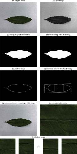
Threshold segmentation: We can separate image to obtain leaf contour through threshold segmentation, which can distinguish the gray value difference between the target leaf area A (mainly green area) and background area B (mainly white area). Therefore, the pixel point gray value greater than the threshold value T was set to I_A, the pixel point gray value smaller than the threshold value T was set to I_B, and the separation of the target area and the background area was achieved. In addition, the threshold-divided image was converted to a binary image. The threshold splits transform function is as follows:

$f(x,y)=\left\{\begin{array}{c}{I}_B,f(x,y)>T\\ I_A,f(x,y)\le T\end{array}\right.$

This study obtained the optimal threshold value T by the method of maximum between class variance (also known as the Otsu method).^[16] The main steps are as follows:

(1) The total number of pixels in the detected image is N, and the maximum gray value of the pixels is L in the leaf gray image. The image gradation value variation range to [0, L-1], and the total number of pixel points in the image with the gradation value i was set to n_i. The initial threshold value T of this study was chosen to be 0.

The pixels of the image were traversed in sequence. In the threshold segmentation function, I_A and I_B were taken as 255 and 0, respectively. Finally, a binary image of the leaf area A (pure white area) having a gray value of 255 and the background area B (pure black area) having a gray value of 0 was obtained. The proportion of two areas that the total number of pixels in the image are determined as follows:

$\left\{\begin{array}{c}{w}_A=\sum _{i=T+1}^{L-1}{n}_i/N\\ w_B=\sum _{i=0}^T{n}_i/N=1-w_A\end{array}\right.$

(2) The average gray values u, u_A, and u_B of the entire image, the target area A, and the background area B are calculated as follows:

$\left\{\begin{array}{c}u=\sum _{i=0}^{L-1}i{n}_i/N\\ u_A=\sum _{i=T+1}^{L-1}i{n}_i/(N{w}_A)\\ u_B=\sum _{i=0}^{T}i{n}_i/(N{w}_B)\end{array}\right.$

Then, the interclass variance in the target area A and the background area B are defined as follows:

${\sigma }^2=w_A(u_A-u{)}^2+w_B(u_B-u{)}^2$

The threshold value T was selected in the range of [0, L-1], the best threshold was determined when the variance between classes was maximum, and the leaf gray image was transformed into the leaf binary image of only two colors: black and white. The leaf target area was filled with black, and the shooting background area was filled with white. The leaf binary image after threshold segmentation is shown in Figure 3(c).

Noise processing

The binary image obtained after the threshold processing often had obvious maximum or minimum value areas due to insufficient shooting light, resulting in the low detection accuracy of chlorophyll content. These problems can be solved by image opening operations.^[17] However, the image processed by the open operation result in the edge of the image was not smooth, and various types of noise affected the image quality and structure. Therefore, we used median filtering to process the blade binary image which can remove the noise and does not affect the main outline of the image, although it will blur the image.^[18] The leaf binary image after the image opening operation and median filtering based on the OpenCV computer vision library are shown in Figure 3(d).

Acquisition of detection model input image

Since the input image of the deep learning network used in this study must be a regular rectangular image. Therefore, the maximum inscribed rectangular area of the leaf contour was selected as the detection image of the deep learning network (About two-thirds of the length of the pomegranate leaves from the bottom to the top). Generally, the chlorophyll content in the edge area of leaves is lower than the average value of chlorophyll in the whole leaf.^[19] Since the chlorophyll values in the middle and edge area of leaves differ greatly. Moreover, the shape of the leaves is irregular, which is harder to perform image processing and deep learning model by taking the whole area of the leaf. However, the chlorophyll values in the central area of leaves change little. Hence, the objective evaluation of the chlorophyll content of the pomegranate leaves is most reasonable through this method.

Maximum inscribed rectangular area of leaf contour extraction

The steps for extracting the maximum inscribed rectangular area of the leaf contour were as follows: (a) extract the leaf contour; (b) acquire the minimum enclosing rectangle of the leaf contour; (c) find the maximum inscribed rectangle of the leaf contour in the minimum enclosing rectangular area of the leaf contour; (d) select the maximum inscribed rectangular area of the leaf image as the chlorophyll content detection area.

The minimum enclosing rectangle of the leaf contour and leaf contour were obtained through the OpenCV computer vision library. Maximum inscribed rectangular area detection was obtained by the central diffusion method.^[20] The leaf contour image, the minimum enclosing rectangle image of that image, and the maximum inscribed rectangle image of that image are shown in Figure 3(e–g), respectively. The maximum inscribed rectangular area acquisition process is shown in Figure 4. And the detail steps for detecting the maximum inscribed rectangular area of the leaf contour are as follows:

Figure 4. Sample diagram of steps for maximum inline rectangular area

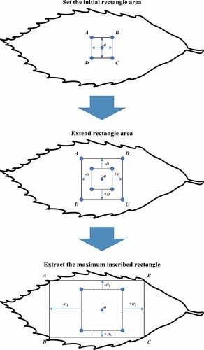
(1) Set the initial rectangle area

Obtain the center point coordinate of the minimum enclosing rectangle of the leaf contour as (centerx, centery) and initialize an inscribed rectangle. The coordinates of the four vertices A, B, C and D of the initialized inscribed rectangle were as follows:

$\left\{\begin{array}{c}Poin{t}_A=(centerx-1,centery-1)\\ Poin{t}_B=(centerx+1,centery-1)\\ Poin{t}_C=(centerx+1,centery+1)\\ Poin{t}_D=(centerx-1,centery+1)\end{array}\right.$

(2) Extend the rectangular area

The four state variables were set to S_AB, S_BC, S_CD, S_DA and initialized to 1. To determine whether the value of all pixels on the line segment AB is 0. If neither was 0, line segment AB was translated by one unit away from the center point. Otherwise, line segment AB was unchanged and state variables S_AB was set to 0. Line segments BC, CD and DA were processed in the same way.

(3) Extract the maximum inscribed rectangle

The line segments AB, BC, CD, DA were cyclically processed to expand the rectangular area until all four state variables were 0. The resulting rectangle ABCD was the maximum inscribed rectangle.

On the one hand, the rectangle is more suitable for the input of deep learning model and saves recognition time. On the other hand, chlorophyll content at different positions of leaves will lead to different RGB values of corresponding pixels. The chlorophyll value of the central area of the leaf is the most representative,^[19] and the rectangular detection area is the central area of the leaf, which ensures the stable and consistent RGB values of the deep learning input image and reduces the error.

Acquisition steps of model input image

The input image of the deep learning network needs a fixed size. However, the image sizes of the maximum inscribed rectangular area obtained by image processing of different leaf images are not consistent. Therefore, the height and width of the image of the maximum inscribed rectangular area of the leaf contour were set to a multiple of 32 with OpenCV, and then the maximum inscribed rectangular area of the leaf contour was equally divided into a plurality of 32 × 32 size subregions. The result is shown in Figure 3(i). When the training set was established, all the divided sub-images were used as training input images, and the corresponding original chlorophyll content was taken as the output. When the detection model was tested, the average of all the sub-images was taken as the final test result.

Results and discussion

Detection model establishment and detection results

Deep learning is the most important breakthrough in artificial intelligence in the past decade and has achieved great success in many fields, such as computer vision, speech recognition, and natural language processing.^[21] The convolutional neural networks commonly used in deep learning require a very large amount of data to build models, while traditional machine learning models have a low detection accuracy.^[22] To address these two problems, this study used the SSAE in deep learning to establish the detection model. The SSAE can still maintain high precision under a small data training model. The SSAE is able to perform unsupervised feature learning on leaf images, and the deep learned features can be used for the regression analysis of chlorophyll content.

Sparse autoencoder

The autoencoder (AE) is an unsupervised learning algorithm that learns identifying features from a large amount of unmarked data. As shown in Figure 5, the AE is a symmetric three-layer neural network. The input data of the AE are as follows:

$X=\{x_{(1)},x_{(2)},x_{(i)},x_{(N)}{\}}^T,x_{(i)}\in R^M$

Figure 5. Autoencoder structure

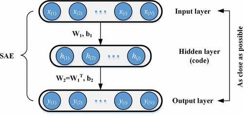
where N is the total number of samples and M is the length of each data sample. The hidden layer output by using the following formula:

$h(x_{(i)},W,b)=\sigma (W{x}_{(i)}+b_1),i=1,\cdots ,N$

Then, the output of the output layer used in this research can be expressed as follows:

$Y=\sigma (W^{T}h(x_{(i)},W,b_2)+c),i=1,\cdots ,N$

The goal of the AE is to make Y= X and then obtain the low-dimensional representation of the input data (hidden layer output $h(x_{(i)},W,b)$). However, due to the limitations of its structure, the AE cannot effectively extract meaningful features even though the AE output can recover the input data well. To obtain more robust features, the sparse autoencoder (SAE) can be constructed by introducing a sparse encoding into the AE. The SAE can improve the performance of the traditional AE and extract more representative low-dimensional concise expressions from high-dimensional raw data.^[23,24] The SAE adds the sparse penalty term to the objective function of the AE, thereby constraining the learned features rather than simply repeating the input.

Sparseness means that when the activation function of the deep learning network is a sigmoid function, the output of the neuron is close to 1 and the neuron is considered activated, whereas the output is considered suppressed when it has a value close to 0.^[25] To obtain sparsity in the AE, the value of each hidden neuron is close to 0, which means that the neurons in the hidden layer are mostly inactive, and AE can represent the characteristics of the input layer with the lowest number (sparse) of hidden units. A sparse penalty term was added to the AE loss function to implement the SAE to achieve this goal. Usually, the KL divergence was applied as a sparse penalty term in the SAE.^[26] However, due to too many parameters of the KL divergence, it is difficult to establish the detection model. Therefore, this study chose L1 regularization as the sparse penalty term instead of KL divergence.

L1 regularization can produce a weight equal to 0 to eliminate certain features, thereby resulting in sparse effects, and it can also avoid overfitting.^[27] Thus, L1 regularization was added to the AE to build a SAE, and the overall loss function of SAE can be expressed as follows:

$J_{sparse}(W,b)=J(W,b)+\beta \sum _{j=1}^s\left|w_j\right|$

where s is the number of hidden layers; β is the sparse weight; and $\sum _{j=1}^s\left|w_j\right|$ is the L1 regularization sparse penalty. The training goal is to minimize the loss function. When the average value of the hidden layer neurons is closer to 0, the sparse penalty is smaller, the model training error is smaller, and the accuracy is higher.

Stacked sparse autoencoder

The stacked sparse autoencoder (SSAE) can be considered a stack of multiple SAEs. The SSAE can extract deep features from complex data, and its training process consists of unsupervised layer-by-layer pretraining and supervised fine-tuning. The overall training process is shown in Figure 6.

Figure 6. Stacked sparse autoencoder structure

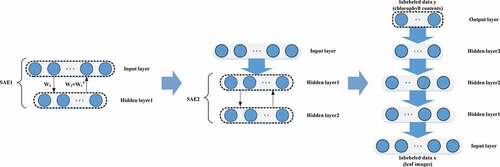
The main difference between SSAE and other deep learning models is unsupervised layer-by-layer training. The SSAE can learn nonlinear complex functions by directly mapping data from inputs to outputs through layer-by-layer learning, which is the key to its powerful feature extraction capabilities. In unsupervised pretraining, the first SAE was trained, the output of the hidden layer of the SAE was taken as the input of the second SAE, and then the second SAE was trained. This process was repeated to achieve layer-by-layer stacking of SAEs, and then the SSAE was established. The method of training the SAE layer by layer avoids the complex operation caused by the overall training of the SSAE, and it can extract features from the original data layer by layer and obtain high-level expressions.

After the unsupervised pretraining was completed, the output layer of the chlorophyll content data was added to the top of the SSAE for the regression analysis. The output layer of the SSAE in this study was a fully connected network with layer numbers 64–1. Finally, the entire network including the output layer was supervised, which means that the BP algorithm was used to fine-tune the relevant parameters of the network to realize the construction of the SSAE.

Data sets and evaluation indicators

The sample set was 4000 image-processed pomegranate leaf images, which were divided into a training set, verification set, and test set according to the proportion of 7:1.5:1.5, respectively. The training set, validation set and test set sample numbers were 2800, 600, and 600 images, respectively. The model performance evaluation index is the sample relative error:

$metrics=\sum _{i=1}^N\left|\left(y_i-{\hat{y}}_i\right)\right|/N$

where N is the total number of samples, ${\hat{y}}_i$ is the chlorophyll content model test value, and $y_i$ is the actual value of chlorophyll content.

Determination of the SSAE structure

Constructed SSAE with hidden layers of 3 to 6 layers to select the appropriate SSAE structure and build the best SSAE model. The number of input and output layer nodes corresponded to the data set the input image size and output image size, respectively. We performed the flattening operation on the input image to obtain the input data of SSAE, which converted the image with 32 × 32 × 3 pixels into one-dimensional data 3072. Therefore, the number of input nodes was 3072, and the number of output nodes was 1. The number of hidden layer neurons was set to different given values, and sparse penalty terms with different sparse weights were added. As shown in Table 1, when the SSAE had four hidden layers, the number of nodes in each layer of the hidden layer was 2048, 1024, 512, and 256, and when $\beta$ was 0.00005, the average relative error was the lowest (5.656%). The SSAE output structure used in this study, including the input layer and the fully connected layer, was 3072-2048-1024-512-256-64-1, and $\beta$ was 0.00005.

Table 1. Validation set results under different SSAE structures

Hidden layers	Number of hidden nodes	0.005	0.001	0.0005	0.0001	0.00005	0.00001
3	2048:1024:256	20.135	20.075	18.690	18.425	16.366	17.614
3	2048:1024:512	17.574	18.635	17.890	15.530	13.360	12.474
4	2048:1024:512:256	12.081	10.959	9.272	7.356	5.656	6.470
4	2250:1500:756:256	12.042	13.547	11.772	10.101	6.561	8.880
5	2048:1500:1024:512:256	13.834	11.447	11.181	6.208	6.274	13.719
6	2250:1500:756:512:256	14.169	14.071	13.192	8.131	9.780	10.763
6	2048:1500:1024:756:512:256	17.361	15.592	16.664	14.524	9.418	8.570
6	2250:1750:1250:756:512:256	19.953	20.008	19.834	15.225	13.206	17.549

Model comparison

It is necessary to prove the validity of the proposed method. The SSAE model was compared with the traditional support vector machine (SVR), random forest (RF), and stacked AE without a sparse penalty based on the test set.^[28–30] These models were trained through the training set, and then the validation set was used for parameter adjustment. Finally, the test set was used to compare the model results. The SVR structure parameters were kernel (rbf), C (300), and gamma (0.01), and other parameters were the sklearn machine learning library default parameters. The RF structure parameter was the number of decision trees (20), and the other parameters were the sklearn machine learning library default parameters. The stacked AE structure parameter was layers (3072-2048-1024-512-256-64-1).

The results are shown in Figure 7. The overall average relative error and the single maximum relative error of the SSAE were 5.796% and 9.167%, respectively; the overall average relative error and the single maximum relative error of the stacked autoencoder were 7.452% and 12.239%, respectively. Here, the results of our model in detecting chlorophyll content are more accurate than those of Asraf et al. in detecting the classification of nitrogen, potassium, and magnesium in oil palm (83%).^[31]

Figure 7. Test results of different models

The error of the SSAE and SAE was much lower than that of the traditional algorithm model (SVR, RF), indicating that the accuracy of using the stacked autoencoder was higher than that of the traditional machine learning model. In addition, the SSAE with the sparse penalty was more accurate than the stacked autoencoder. The overall average relative error and the single maximum relative error of the SSAE were reduced by 1.656% and 3.072%, respectively, which indicated that the addition of sparse penalties to the SSAE was effective.

In the actual test, SSAE network training required a longer amount of time than the other model methods, although when the trained SSAE network was used for sample prediction, one sample prediction per second was completed, which is a high rate in real-time performance. Thus, the high-precision SSAE network for the detection of chlorophyll content is of great significance for precise fertilization and management of orchards.

Conclusion

The article proposed a plant chlorophyll content estimation method based on digital image processing technology and a SSAE deep learning model. The central area of the leaf image was extracted by digital image processing technology as the detection target, and the powerful representation ability and overall network fine-tuning mechanism of the SSAE network were used for modeling. The method greatly reduces the time for manual processing of data and achieves a highly precise chlorophyll content prediction, thus increasing the intelligence and efficiency of chlorophyll content prediction. The detection image was extracted by image analysis, and the prediction model based on the SSAE could learn the deep-seated features of the data. Moreover, our model was more effective than other traditional image prediction methods for chlorophyll content prediction.

Additional information

Funding

This work was supported by the Doctorate Fellowship Foundation of Nanjing Forestry University (163010550), and the Priority Academic Program Development of Jiangsu High Education Institutions (PAPD).

References

- Arregui, L. M.; Lasa, B.; Lafarga, A.; Iraneta, I.; Baroja, E.; Quemada, M. Evaluation of Chlorophyll Meters as Tools for N Fertilization in Winter Wheat under Humid Mediterranean Conditions. Eur. J. Agron. 2006, 24, 140–148. DOI: 10.1016/j.eja.2005.05.005.
- Pagola, M.; Irigoyen, I.; Bustince, H.; Barrenechea, E.; Aparicio-Tejo, P.; Lamsfus, C.; Lasa, B. New Method to Assess Barley Nitrogen Nutrition Status Based on Image Colour Analysis. Comput. Electr. Agric. 2009, 65, 213–218. DOI: 10.1016/j.compag.2008.10.003.
- Vibhute, A.; Bodhe, S. K. Color Image Processing Approach for Nitrogen Estimation of Vineyard. Inter. J. Agric. Sci. Res. 2013, 3, 189–196. DOI: 10.1016/S0007-0785(94)80025-1.
- Pierce, F. J.; Nowak, P. Aspects of Precision Agriculture. Adv. Agron. 1999, 67, 1–85. DOI: 10.1016/S0065-2113(08)60513-1.
- Amaral, E. S. D.; Silva, D. V.; Anjos, L. D.; Schilling, A. C.; Andrea-Carla, D.; Mielke, M. S. Relationships between Reflectance and Absorbance Chlorophyll Indices with Rgb (red, Green, Blue) Image Components in Seedlings of Tropical Tree Species at Nursery Stage. New For. 2018, 1–12. DOI: 10.1007/s11056-018-9662-4.
- Noh, H.; Zhang, Q.; Shin, B.; Han, S.; Feng, L. A Neural Network Model of Maize Crop Nitrogen Stress Assessment for A Multi-spectral Imaging Sensor. Biosyst. Eng. 2006, 94, 477–485. DOI: 10.1016/j.biosystemseng.2006.04.009.
- Su, C. H.; Fu, C. C.; Chang, Y. C.; Nair, G. R.; Ye, J. L.; Chu, I. M.; Wu, W. T. Simultaneous Estimation of Chlorophyll a and Lipid Contents in Microalgae by Three-color Analysis. Biotech. Bioengin. 2010, 99, 1034–1039. DOI: 10.1002/bit.21623.
- Liu, P.; Shi, R.; Zhang, C.; Zeng, Y.; Wang, J.; Tao, Z.; Gao, W. Integrating Multiple Vegetation Indices via an Artificial Neural Network Model for Estimating the Leaf Chlorophyll Content of Spartina Alterniflora under Interspecies Competition. Environ. Monitor. Assess. 2017, 189, 596. DOI: 10.1007/s10661-017-6323-6.
- Gaviria-Palacio, D.; Guaqueta-Restrepo, J. J.; Pineda-Tobon, D. M.; Perez, J. C. Fast Estimation of Chlorophyll Content on Plant Leaves Using the Light Sensor of a Smartphone. Dyna. 2017, 84, 234–239.
- Gupta, S. D.; Pattanayak, A. K. Intelligent Image Analysis (iia) Using Artificial Neural Network (ann) for Non-invasive Estimation of Chlorophyll Content in Micropropagated Plants of Potato. In Vitro Cell.r Develop. Bio. Plant. 2017, 14, 1–7. DOI: 10.1007/s11627-017-9825-6.
- Sulistyo, S. B.; Wu, D.; Woo, W. L.; Dlay, S. S.; Gao, B. Computational Deep Intelligence Vision Sensing for Nutrient Content Estimation in Agricultural Automation. IEEE Trans. Autom. Sci. Eng. 2017, 15(3), 1243–1257. DOI: 10.1109/TASE.2017.2770170.
- Yadav, S. P.; Ibaraki, Y.; Gupta, S. D. Estimation of the Chlorophyll Content of Micropropagated Potato Plants Using Rgb Based Image Analysis. Plant Cell Tissue Organ. Cul. 2010, 100, 183–188. DOI: 10.1007/s11240-009-9635-6.
- Gago, J.; Martinez-Nunez, L.; Landin, M.; Gallego, P. P. Artificial Neural Networks as an Alternative to the Traditional Statistical Methodology in Plant Research. J. Plant Physiol. 2010, 167, 23–27. DOI: 10.4161/psb.5.6.11702.
- Vesali, F.; Omid, M.; Kaleita, A.; Mobli, H. Development of an Android App to Estimate Chlorophyll Content of Corn Leaves Based on Contact Imaging. Comput. Electron. Agric. 2015, 116, 211–220. DOI: 10.1016/j.compag.2015.06.012.
- Zhang, M.; Gunturk, B. K. Multiresolution Bilateral Filtering for Image Denoising. IEEE Trans. Image Process 2008, 17, 2324–2333. DOI: 10.1109/TIP.2008.2006658.
- Otsu, N. A Threshold Selection Method from Gray-level Histograms. IEEE Trans. Syst. Man Cybern. 2007, 9, 62–66. DOI: 10.1109/TSMC.1979.4310076.
- Gonzalez, R. C.; Woods, R. E. Digital Image Processing, 3rd ed. Prentice-Hall: Upper Saddle River, USA, 2008; pp. 636. ISBN 978-0131687288. DOI:10.1109/IEMDC.2013.6556306.
- Huang, T.; Yang, G.; Tang, G. A Fast Two-dimensional Median Filtering Algorithm. IEEE Trans. Acoustic. Speech. Sign. Process. 1979, 27, 13–18. DOI: 10.1109/TASSP.1979.1163188.
- Yuan, Z.; Cao, Q.; Zhang, K. Syed Tahir Ata-Ul-Karim, Yongchao Tian, Yan Zhu, Weixing Cao, and Xiaojun Liu. Optimal Leaf Positions for SPAD Meter Measurement in Rice. Front. Plant Sci. 2016, 7, 719.
- Fischer, P.; HFfgen, K. U. Computing a Maximum Axis-aligned Rectangle in a Convex Polygon. Inf. Process. Lett. 1994, 51, 189–193. DOI: 10.1016/0020-0190(94)00079-4.
- Lecun, Y.; Bengio, Y.; Hinton, G. Deep Learning. Nature. 2015, 521, 436–449. DOI: 10.1038/nature14539.
- Miotto, R.; Wang, F.; Wang, S.; Jiang, X.; Dudley, J. T. Deep Learning for Healthcare: Review, Opportunities and Challenges. Briefings Bioinf. 2017, 1–11. DOI: 10.1093/bib/bbx044.
- Wright, J.; Ma, Y.; Mairal, J.; Sapiro, G.; Huang, T. S.; Yan, S. Sparse Representation for Computer Vision and Pattern Recognition. Proc. IEEE. 2010, 98, 1031–1044. DOI: 10.1109/jproc.2010.2044470.
- Sun, W.; Shao, S.; Zhao, R.; Yan, R.; Zhang, X.; Chen, X. A Sparse Auto-encoder-based Deep Neural Network Approach for Induction Motor Faults Classification. Measurement. 2016, 89, 171–178. DOI: 10.1016/j.measurement.2016.04.007.
- Bourlard, H.; Kamp, Y. Auto-association by Multilayer Perceptrons and Singular Value Decomposition. Biol. Cyber. 1988, 59, 291–294. DOI: 10.1007/bf00332918.
- Kullback, S.; Leibler, R. A. On Information and Sufficiency. Ann. Math. Stats. 1951, 22, 79–86. DOI: 10.1214/aoms/1177729694.
- Balamurugan, P.; Shevade, S.; Babu, T. R. Scalable Sequential Alternating Proximal Methods for Sparse Structural Svms and Crfs. Know. Inf. Syst. 2014, 38(3), 599–621. DOI: 10.1007/s10115-013-0681-3.
- Hong, W. C. Electric Load Forecasting by Seasonal Recurrent Svr (support Vector Regression) with Chaotic Artificial Bee Colony Algorithm. Energy. 2011, 6, 5568–5578. DOI: 10.1016/j.energy.2011.07.015.
- Ibarra-Berastegi, G.; Saenz, J.; Esnaola, G.; Ezcurra, A.; Ulazia, A. Short-term Forecasting of the Wave Energy Flux: Analogues, Random Forests, and Physics-based Models. Ocean Eng. 2015, 104, 530–539. DOI: 10.1016/j.oceaneng.2015.05.038.
- Xu, J.; Xiang, L.; Liu, Q.; Gilmore, H.; Wu, J.; Tang, J.; Madabhushi, A. Stacked Sparse Autoencoder (ssae) for Nuclei Detection on Breast Cancer Histopathology Images. IEEE Trans. Med. Imaging. 2016, 35, 119. DOI: 10.1109/ISBI.2014.6868041.
- Asraf, M. H.; Dalila, N. K.; Faiz, A. Z.; Aminah, S. N.; Nooritawati, M. T. A Fuzzy Inference System for Diagnosing Oil Palm Nutritional Deficiency Symptoms. ARPN J. Engg. Appl. Sci. 2017, 12(10), 3244–3250.