Assessing the spatial distribution of nitrogen dioxide in London, Ontario

Abstract

Land use regression (LUR) models have been widely used to characterize the spatial distribution of urban air pollution and estimate exposure in epidemiologic studies. However, spatial patterns of air pollution vary greatly between cities due to local source type and distribution. London, Ontario, Canada, is a medium-sized city with relatively few and isolated industrial point sources, which allowed the study to focus on the contribution of different transportation sectors to urban air pollution. This study used LUR models to estimate the spatial distribution of nitrogen dioxide (NO₂) and to identify local sources influencing NO₂ concentrations in London, ON. Passive air sampling was conducted at 50 locations throughout London over a 2-week period in May–June 2010. NO₂ concentrations at the monitored locations ranged from 2.8 to 8.9 ppb, with a median of 5.2 ppb. Industrial land use, dwelling density, distance to highway, traffic density, and length of railways were significant predictors of NO₂ concentrations in the final LUR model, which explained 78% of NO₂ variability in London. Traffic and dwelling density explained most of the variation in NO₂ concentrations, which is consistent with LUR models developed in other Canadian cities. We also observed the importance of local characteristics. Specifically, 17% of the variation was explained by distance to highways, which included the impacts of heavily traveled corridors transecting the southern periphery of the city. Two large railway yards and railway lines throughout central areas of the city explained 9% of NO₂ variability. These results confirm the importance of traditional LUR variables and highlight the importance of including a broader array of local sources in LUR modeling. Finally, future analyses will use the model developed in this study to investigate the association between ambient air pollution and cardiovascular disease outcomes, including plaque burden, cholesterol, and hypertension.

Implications:

Monitoring and modeling of NO₂ throughout the city of London represents an important step toward assessing air pollution health effects in a mid-sized Canadian city. The study supports the introduction of railways to LUR modeling of NO₂. Railways explained approximately 9% of the variability in ambient NO₂ concentrations in London, which suggests that local sources captured by land-use indicators may contribute to the efficacy of LUR models. These findings provide insights relevant to other medium and smaller sized cities with similar land use and transportation infrastructure. Furthermore, London is a central hub for medical research and treatment in southwestern Ontario, with facilities such as the Robarts Research Institute, London Regional Cancer Program (LRCP), and Stroke Prevention & Atherosclerosis Research Centre (SPARC). The models developed in this study will provide estimates of exposure for future analyses examining air pollution health effects in this data-rich population.

Introduction

Exposure estimation can have significant impacts on explaining relationships between air pollution and adverse health outcomes (Ryan et al., 2007; Fischer et al., 2000; Linaker et al, 2000). Consequently, there is a growing demand for improved and affordable exposure estimation to capture the variability of intra-urban air pollution for health studies (International Society of Exposure Science, 2011; Jerrett et al., 2007; Fung et al., 2007). Various approaches have been proposed and utilized to address the challenges of estimating residential and neighbourhood level exposure concentrations. For example, kriging has been used at both the national and regional scale (Hoek et al., 2008), but is limited by its inability to capture the numerous intersecting line sources and rapid distance decay of air pollution at intra-urban scales (Briggs et al., 1997). Other studies have used proximity analysis (distance to known sources of pollution such as industry and traffic) or community-level pollution concentrations as proxies for exposure (Dockery and Stone, 2007; Burnett et al., 2004; Pope et al., 2002). However, these approaches are limited by their high potential for exposure misclassification (Jerrett et al., 2007).

Personal and household-level monitoring provide more accurate measures of exposure (Levy et al., 2000), but the suitability of individual monitoring for estimating exposure in epidemiologic studies is hampered by the high cost and participant burden associated with air monitoring data collection, particularly for a large cohort (Madsen et al., 2007). Dispersion models have also been used to estimate exposure because they incorporate both spatial and temporal variations in pollutant concentration; however, dispersion models require resource-intensive meteorological and emissions data to make accurate predictions (Briggs et al., 1997; Jerrett et al., 2005). Land use regression (LUR) modeling has emerged as a cost-effective alternative approach to meet these challenges of assessing the intra-urban spatial variability of ambient air pollutants in urban and industrial settings because it can capture local-scale spatial variations more effectively and economically than previous monitoring and modeling approaches (Ryan et al., 2007; Levy et al., 2000; Jerrett et al., 2005; Brauer et al., 2003).

LUR modeling predicts outdoor ambient air pollution concentrations using widely available geographic information system (GIS)-based land use characteristics (e.g., traffic, population, and dwelling density) and physical environmental features (e.g. elevation). Several reviews of LUR studies havedescribed the utility of the method in estimating exposure to air pollution (Hoek et al., 2008; Jerrett et al., 2005; Ryan and LeMasters, 2007). Compared to other geo-statistical methods such as kriging and dispersion modeling, LUR provides higher spatial resolution of variability in urban settings with less data input than dispersion models and lower costs than microenvironmental monitoring (Jerrett et al., 2005). However, while the methodology has proven reliable and effective, only a small number of studies to date have used LUR models to estimate NO₂ concentrations in small and mid-sized cities (Luginaah et al., 2006; Atari et al., 2008; Wheeler et al., 2008).

As a component of a larger research program to examine the impact of ambient pollution on chronic diseases by Health Canada and Environment Canada, this work is aimed at conducting a land use regression (LUR) analysis to characterize the spatial distribution of NO₂ and provide estimates of exposure to air pollution for future health studies in London, Ontario.Burnett et al. (1998) found that among 11 of the most populous urban centers in Canada, London had the highest increased risk of death (9.9%) attributable to change in NO₂ concentrations and second highest risk (9.1%) attributable to change in all pollutants from 1980 to 1991 (carbon monoxide [CO], NO₂, sulfur dioxide [SO₂], and ozone [O₃]). Furthermore, this study contributes to the growing literature describing the utility of LUR for exposure estimation in cities where extensive monitoring campaigns are not feasible. Recent research on the utility of LUR modeling of NO₂ for epidemiological studies has investigated the transferability of models between Vancouver (BC, Canada), Victoria (BC, Canada) and Seattle (WA, United States) (Poplawski et al., 2009), and between Winnipeg (MB, Canada) and Edmonton (AB, Canada) (Allen et al., 2011). Results from this study supports transferability objectives by examining how land use and transportation infrastructure characteristics in a mid-size city contribute to NO₂ concentrations.

Methods

The LUR model development in the current study was similar to approaches used byJerrett et al. (2007) and Kanaroglou et al. (2005) and involved development of a location-allocation model for choosing optimal monitoring locations (Buzzelli, 2008); deployment of air pollution monitors and measurement of pollution concentrations in locations in and around the City of London; and the application of LUR modeling to examine land use characteristics that contribute to NO₂ variability in London. The LUR model is subsequently used to estimate ambient concentrations throughout the city based on these land use characteristics.

Study area

The London census metropolitan area (42° 59′ 00″ N; 81° 14′ 00″ W) has a population of 366,151, with an approximate area of 420.57 km² (Statistics Canada, 2012). Land use features in London (Figure 1) are representative of small and mid-sized cities in North America. These include the dominating presence of railway infrastructure in central areas of the city, and lack of a controlled-access highway or thoroughfare for local traffic. Two expressways transect London, but they are located at the southern periphery of residential settlement. The city's location within the most industrialized region of Canada and proximity to cities like Sarnia and Windsor with documented air pollution health problems (Oiamo et al., 2011; Luginaah et al., 2005) are causes of concern to local residents, officials, and public health professionals. London is located in the busiest trade corridor between the United States and Canada, as well as downwind from point sources such as oil refineries, steel mills, and coal plants in Michigan and southwestern Ontario. The city is noted for its economic diversity and is the home to many branches of industry, corporate offices, and medical and educational facilities. It is also a manufacturing, distribution, and financial center in southwestern Ontario.

Figure 1. Map showing the 50 monitoring sites, land use categories, highways, railway, and Ministry of Environment (MOE) monitoring station in London, ON.

Air pollution monitoring of NO₂

Ogawa passive samplers (Ogawa & Company USA, Inc., Pompano Beach, FL) were used to measure the ambient nitrogen dioxide (NO₂) concentrations. The 2-week sampling period was from May 31 to June 14, 2010. Fifty monitoring sites (Figure 1) were selected based on a location-allocation model (LAM) for which the p-median (P-MP) approach was used. The goal of LAMs in general is to select n candidate locations taking into account demand attributed to those locations. In this case, demand at candidate locations was represented by preliminary estimates of NO₂ concentrations and proportions of residents aged 40 years or more. The P-MP approach minimizes the sum of the distance between all demand locations and chosen sampler locations. In other words, this approach provides an efficient model of spatial coverage for sampling air pollution (Kanaroglou et al, 2005). Demands were created on a surface grid with 500-m² parcels and used as weights in the LAM algorithm that placed 50 monitors at a minimum distance of 1500 m from each other throughout London.

Monitors were installed on light poles, with permission from the City of London, as close as possible to the LAM sites at a height of 3 m to prevent contamination and vandalism. One site was collocated with the only Ontario Ministry of the Environment (MOE) monitoring site in London, which is also part of Environment Canada's National Air Pollution Surveillance (NAPS) network. Stainless-steel rain shelters were used to protect the samplers from inclement weather. The planned setup was on Monday May 31; however, due to an afternoon thunderstorm only 47 out of the 50 sites were set up. The remaining three sites were set up the following day, June 1, and there were no observable anomalies between monitors set up before or after the storm. The take-down for all sites took place on Monday, June 14. Hourly temperature and relative humidity data from the London Airport (Environment Canada, 2010) were averaged during the weeks for the study area to calculate NO₂ concentration conversion coefficients. The average temperature and relative humidity during the study period were 18°C and 80%. A global positioning system receiver was used to geocode all of the monitoring sites.

All sites yielded valid samples with no samples lost due to tampering or vandalism incidents. The exposed NO₂ filters were analyzed by Environment Canada (Egbert, Ontario) according to the Ogawa protocol (Ogawa & Co, 2006). Field blanks, which constituted 10% of total samples (n = 5), were deployed to quantify the sample mass attributable to handling and transportation. Field duplicates (n = 5) were used to assess the precision of the method. This was calculated using a non-bias % difference formula ( eq 1). If the difference was less than 15%, the average of the two was taken as the final result; if the difference was greater than 15% the individual concentrations of each duplicate was examined versus all filters.

1

All NO₂ concentration results were corrected using the field blanks at the nanograms per filter level. Two batch blanks were prepared and their concentration was compared to the mean value of the field blanks. The estimated bias of the sampling methodology was calculated as the fractional difference between the NAPS data and collocated sampler (Bias = (S – T)/T; S is the sample value and T is the true value based on standardized method used by MOE). The formula used to calculate the final NO₂ concentrations (ppb) was provided by Ogawa & Company (2006).

Land use and spatial data

Potential predictors were extracted from multiple datasets (described next) and conceptually grouped into four categories: land use, transportation, population and dwellings, and physical environmental features (Table 1).

Table 1. Categories and corresponding variables considered for inclusion in the LUR model

	Buffer radius in meters (intervals)
Landuse
Industrial area (ha)	200–1600 (200)
Open area and water (ha)	200–1600 (200)
Residential area (ha)	200–1600 (200)
Commercial area (ha)	200–1600 (200)
Transportation
Distance to nearest major  road (km)	n/a
Distance to nearest highway (km)	n/a
Traffic density	50–1000 (50)
Length of major road within buffer (km)	50–1000 (50)
Length of Highway (km)	50–1000 (50)
Length of railway (km)	50–750 (50)
Population and dwelling
Population density within buffer	100–1500 (100)
Dwelling density within buffer	100–1500 (100)
Physical feature
Elevation (m above sea level)	n/a

Land use data sets were obtained from Desktop Mapping Technologies, Inc. (DMTI), via the Data Liberation System from the University of Western Ontario. Land use category variables were calculated as the proportional area of land use (industrial, commercial, institutional, residential, open areas, and water) that fell within the area of the specified buffer distances ranging from 200 m to 1600 m at 200-m intervals. The street network file had information on all three types of roads (minor, major, and highways) and railways. Variables for the transportation category included calculated lengths of major roads and highways within buffer distances from 50 m to 1000 m at 50-m intervals. Calculated distances (km) from each monitoring site to the nearest major road and highway were also included as variables. Variables for railway were calculated at the same buffer distances as highways by adding the lengths of track within the buffer. Note that train depots have multiple tracks that increased the magnitude of calculated track lengths in those areas.

Annual average daily traffic (AADT) data collected in 2005 was obtained from the City of London, and street network data sets were obtained from DMTI. The 2005 data was in the format of a road layer, and each road segment was associated with a traffic count value. A line density function was used to calculate traffic density. Raster data are stored as pixels or cells in ArcGIS, and were therefore utilized to create a grid surface with 5 × 5-m cells. A circle was drawn around each cell center using different radii (50–1000 m) to generate traffic density variables at each radius. The length of a road segment that fell within each circle was multiplied by its daily traffic count value. These figures were summed and the total divided by the circle's area to get the traffic density for the circle. Therefore, actual traffic density values provide an index rather than specific units (Sahsuvaroglu et al., 2006). All variables were generated using ArcGIS 9.2 (ESRI, Redlands, CA).

Variables for population density in addition to dwelling density were included in the analysis to determine whether there was an effect of household characteristics on NO₂ concentrations. Population density can differ from dwelling density with varying numbers of household members in certain areas, and this may influence the number of vehicles and traffic volumes. Population and dwelling unit counts at the dissemination area (DA) level were generated from 2006 Census data (Statistics Canada, 2007). Dissemination areas respect the boundaries of census subdivisions and census tracts. The boundaries normally follow roads, but may follow other features such as railways or water features where these features form part of the boundaries of census subdivisions or census tracts. The DA is the smallest geographic unit for which Census data are disseminated and has a population of 400 to 700. The variables used in the analysis were created by first calculating the proportion of each DA within a specified buffer radius around the monitoring site. Population and dwelling densities were then calculated by multiplying these proportions by total population or dwelling unit counts of the respective DAs within the buffer and dividing the sum of these products by the buffer area. A key assumption was that individual DAs had uniform population and dwelling densities. Dwelling density and population density were calculated at buffer radii ranging from 100 m to 1500 m at 100-m intervals from the monitor.

The coordinates of each monitoring location were used to generate elevation based on Ontario Ministry of Natural Resources Digital Elevation Model (DEM) data. Temperature and relative humidity were included in calculating the observed concentrations from samplers, but no other meteorological data were included in the LUR models. Variables indicating wind direction have been included in other LUR studies, but were not used in this analysis because Environment Canada's Weather Office reports wind direction and speed for London based on an outlying location of the study area. The weather in this location during the monitoring period was mostly cloudy with a variable calm or light easterly breeze (0–11 kph), or a gentle or moderate northwesterly breeze (12–29 kph). Precipitation exceeding 10 mm was observed on two nonconsecutive days throughout the period. These conditions suggest that the observed and estimated concentrations were not significantly affected by wind or precipitation.

Land use regression model development

Measured ambient concentration of NO₂ was used as the dependent variable. Potential predictors were individually screened using bivariate regression analysis to identify variables from each of the categories associated with measured NO₂. These variables were subsequently included in a stepwise multiple ordinary least squares (OLS) regression procedure to develop the LUR model. The stepwise procedure sequentially identified predictor variables from each category with regression coefficients significantly different from zero (t-test, p < 0.05) by backward elimination. Independent variables included in the final regression models were also tested for collinearity with variables from other categories (variance inflation factor <2). Several iterations with different categorical orders of the resulting subset of independent variables were analyzed using stepwise regression to optimize the coefficient of determination (R ²) in the OLS regression.

All candidate models were tested for outliers and spatial autocorrelation using Moran's I (MI) statistic (Odland, 1988; Griffith, 1987). The final LUR model was the model with the highest overall adjusted R ², no spatial autocorrelation and no significant outliers. The Breusch–Pagan/Cook–Weisberg test was used to assess homoscedasticity in the model (Lyon and Tsai, 1996), and the individual influence of each measured concentration on the whole model was examined using the size-adjusted Cook's distance statistics (Hamilton, 1992). Jackknife variance estimation was used to test the final model parameters for bias and sensitivity among sampling locations (Ryan et al., 2007; Moore et al., 2007). The delete-one jackknife method recalculates the regression coefficients by leaving out each monitor once and comparing it to estimates based on the remaining monitor data (n = 49).

Independent variables in the final LUR model were used to estimate intra-urban NO₂ concentrations throughout London. Raster surfaces were generated for each variable in the NO₂ model using the LUR model equation. The surfaces were then multiplied with their respective coefficients and added using the GIS Raster calculator function in ArcGIS 9.2 to generate the surface NO₂ concentration.

Results

Values of NO₂ observed at the 50 monitoring sites ranged from 2.8 to 8.9 ppb, with a median of 5.2 ppb and an arithmetic mean of 5.4 ppb (SD = 1.3). The batch blanks registered negligible concentrations, which suggested that the sampling medium was free of contamination. Duplicate analysis was conducted to 4 pairs of field samples (one duplicate filter was damaged) and the per cent difference between each pair was calculated. The results of the standards and duplicate analysis showed consistency in the analytical methods used as the percent difference ranged from 3% to 12% with a mean of 5%. This was comparable to the duplicate precision of sampling conducted in Windsor, Ontario (7%) and Quebec City, Quebec (4.5%) (Wheeler et al., 2011; Gilbert et al., 2006). The MOE station mean for the monitoring period was 5.5 ppb, while the average concentration based on the collocated monitor was 5.7 ppb.

The mean observed concentration from our monitors (5.4 ppb) was not significantly different than the MOE station mean (t = –0.29, df = 14, p = 0.77), which indicated that the reference method used by the MOE at their only monitoring station in London is representative of mean NO₂ concentrations for the city. An estimated bias of 3.6% was calculated as the fractional or percent difference between the Ogawa and MOE collocated samplers. The yearly average recorded at the London station in 2010 was 8.83 ppb, with a maximum recording of 68 ppb on March 8. The month of June had the lowest mean levels of NO₂ (5.4 ppb) while November had the highest monthly levels (13.2 ppb). The observed NO₂ concentrations in this study represented a seasonal low, which is a trend reflected throughout southern Ontario (Wallace and Kanaroglou, 2008). Therefore, our observed values provided a conservative estimate of annual NO₂ levels in London.

Table 2 shows the final LUR model. These five variables explained 78% of the variability of observed ambient NO₂ concentrations in London. The significant variables in the model were industrial areas within 1600m, distance to highway, traffic density within 150 m, dwelling density within 1000 m, and length of railways within 550 m. Partial coefficients of determination for the individual variables indicated that traffic density was the most important predictor (partial R²  = 0.60) of NO₂ in our model. Distance to highway reduced the unexplained variation by 17%, followed by dwelling density (15%), industry (10%), and railways (9%). As expected, all variables except distance from highway were positively associated with NO₂ levels. Semi partial coefficients of determination indicated that shared variation among the independent variables explained 0.30 of the total adjusted R² (0.76) for the LUR model.

Table 2. LUR model and cross-validation results for NO₂ based on 50 monitoring locations (R ² = 0.784; adjusted R ² = 0.760)

	Coeff.	Standardized coeff.	Partial R^2	OLS t-value	P > t	Jackknife t-value	P > t	VIF
Intercept				12.03	0.000	13.10	0.000
Industrial land use (1600m)	0.00361	0.201	0.097	2.17	0.035	2.38	0.021	1.754
Length of railways (550m)	0.45028	0.147	0.086	2.03	0.048	2.02	0.049	1.069
Distance to highway	–0.13267	–0.265	0.165	–2.95	0.005	–3.47	0.001	1.647
Traffic density (150m)	0.01412	0.644	0.608	8.26	0.000	6.15	0.000	1.238
Dwelling density (1000m)	2.14373	0.223	0.147	2.75	0.009	2.92	0.005	1.340
Note: VIF, variance inflation factor.

Model diagnostics

Figure 2a shows the observed versus the predicted NO₂ concentration based on the final LUR model, while Figure 2b shows the observed NO₂ concentrations versus their standardized residuals. These plots demonstrate that the LUR model fit the observations well with no influential outliers. The Breusch–Pagan/Cook–Weisberg test was used to test for constant variance and the result indicated that heteroskedasticity was not a problem in the LUR model. The Pearson correlation coefficients between measured and LUR modeled NO₂ concentration at the sampling locations was 0.885 (p < 0.001).

Figure 2. (a) Observed versus predicted NO₂ concentrations based on final LUR model. (b) Observed NO₂ versus standardized residuals from LUR model.

The root mean squared error (RMSE) of 0.65 ppb had a bias-corrected bootstrap confidence interval of 0.58–0.79 after 999 replications. Table 2 presents the jackknife cross-validation parameters, which indicated that the estimates were fairly robust. The change in t-values implied that traffic density was more sensitive to sampling locations than the other predictors. This was likely because the relatively small buffer (150 m) was not able to fully capture the contribution of traffic in areas where characteristics such as dwelling density and industrial density were indirect indicators of traffic pollution. This was confirmed by the reduced variance of these indicators following cross-validation.

Predicted NO₂ concentrations

The LUR surface (Figure 3) showed higher concentrations of NO₂ in the downtown core and industrial areas south and northeast of the city center, and along highways, major roads and railways throughout the city. Higher levels of NO₂ were also predicted along King's Highway 401 east of its junction with Highway 402. This is where traffic joins from the highways leading to Sarnia and Windsor, two major United States–Canada trade corridors. The predicted concentrations also reflect the presence of industrial clusters in the northeast, as well as south London where industrial land use coincides with Highway 401 and railways. Railways that serve both local industries and national transportation networks transect these areas as well as the downtown core.

Figure 3.LUR model surface for NO₂ in London, Ontario.

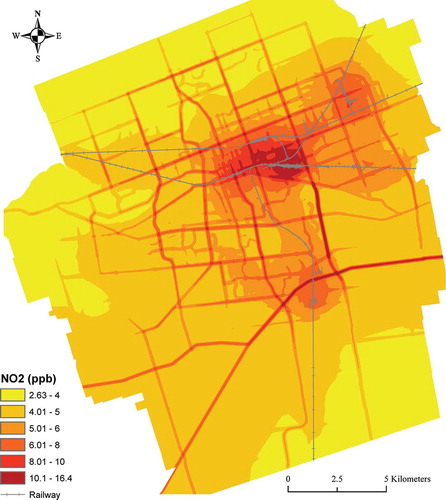
One portion of the railway that joins two lines in the northeast serves a major industrial complex in London where products include diesel locomotives. This area is zoned for light and general industrial use, and therefore showed little or no contribution from dwelling density. Railway tracks in south London likewise transect an industrialized area, but also terminate at a large production facility for food and industrial additives. Railways as a predictor of NO₂ in these regions of the city were coincident with industrial and commercial land uses, which historically developed in areas that could access railway transportation networks. However, two clusters of railway tracks located in the downtown area are Canadian Pacific (CP) and Canadian National (CN) Railway marshaling yards for intermodal and non-intermodal rail traffic through eastern Canada and the United States. Neither yard serves as an intermodal terminal for the respective railways, but municipal zoning and land use planning has led to a cluster of industrial and commercial activity surrounding the CN yard. This area, which is also adjacent to heavily trafficked thoroughfares and residential neighbourhoods, coincided with the highest surface predicted concentrations of NO₂ (16.2 ppb) in London.

Discussion

This study developed an LUR model to characterize intra-urban variation of ambient NO₂ in London, Ontario. This spatially resolved surface for NO₂ incorporated features of the local environment that are significant contributors to air pollution and explained 78% of the variability in ambient NO₂ in London. Finally, the NO₂ surface developed in this study will be applied to estimate exposure to air pollution in future health studies.

Mean NO₂ concentrations in London (5.4 ppb) were lower than Windsor (9.5 ppb), for the same season, but Wheeler et al. (2008) also monitored pollution in the summer, winter and fall seasons. They found that NO₂ concentrations during the spring were lower than other seasons and the yearly average (Wheeler et al., 2008). However, the study also found that spring concentrations had the highest correlation coefficient (Pearson's r = 0.97, p < 0.0001) of all seasons with respect to the yearly mean. This suggests that the London LUR model is highly representative of spatial NO₂ variability throughout the year.

The variation in NO₂ explained by the LUR model was comparable to results for other cities in southern Ontario. The coefficients of determination for NO₂ in southern Ontario cities ranged from 0.69 in Toronto to 0.88 in Windsor (Table 3), and a combination of contextual and conventional indicators of NO₂ optimized the predictive power of these LUR models.

Table 3. Comparison of NO₂ land use regression variables for different cities in Ontario

	Sarnia ^1	Windsor ^2	Hamilton ^3	Toronto ^4	London
Land use categories	Industry 1600 m	Industry 600 m	Industry 200 m	Industry 750 m	Industry 1600 m
	—	—	Open 500 m	—
	—	—	Downtown industrial core	—	—
Roads and traffic	Highways 400 m	—	Highways 50 m	Highways 200m	Distance to highway 401/402
	—	—	—	Major roads 50m	—
	—	Traffic density on C1 roads 400 m	Traffic density 300 m	Traffic density 500 m	Traffic density 150 m
	—	Traffic density on C2 roads 400 m	—	—	—
Railways	—	—	—	—	Length of tracks within 550m
Population and dwelling density	Dwelling density within 2400 m	Sum of population within 700 m	—	Dwelling density 2000 m	Dwelling density within 1000 m
Geographic location	Distance to industrial core	Distance to Ambassador Bridge	Distance to Lake Ontario	X (longitude)	—
Wind	Not used	Not used	Downwind of highway 403	Downwind of all highways 1500 m	Not used
Study area ^a	165 km^2	145 km^2	1372 km^2	633 km^2	422 km^2
Population size	71,419	208,000	660,000	2.6 million	1.6 million
R ^2	0.79	0.88	0.76	0.69	0.784
Number of samplers	39	50	107	100	50
Notes: Sources: ^1 Atari et al. (2008); ^2 Luginaah et al. (2006); ^3 Sahsuvaroglu et al. (2006); ^4Jerrett et al. (2007).
^aBased on city area except for Hamilton, which is based on census metropolitan area.

Several predictors in the London LUR model were also significant in NO₂ models developed for nearby cities in southern Ontario. Table 3 compares the independent variables from LUR models in Sarnia (Atari et al., 2008), Windsor (Luginaah et al., 2006), Hamilton (Sahsuvaroglu et al., 2006), Toronto (Jerrett et al., 2007), and London. Industrial land use and traffic related variables were significant indicators of NO₂ in all LUR models, although the studies differed with respect to buffer distances for industry and roadways, in addition to their measures of traffic density. The models developed in London and Sarnia both include industry within 1600 m as a significant indicator, but this variable predicted 48% of NO₂ variation in Sarnia compared to 10% in London. An additional 20% of NO₂ variance in Sarnia was predicted by distance to the industrial core, whereas length of highway within 400 m was the only traffic related variable, predicting 6% of variation. For LUR models in Hamilton, industrial land use and proximity to the industrial core were significant predictors, though weaker indicators of NO₂ than traffic.

In the LUR model for London, Ontario, road and traffic related variables predicted 55% of observed NO₂ concentrations. This was consistent with LUR models for other cities in southwest Ontario in which road and traffic variables were significant predictors. In Windsor, distance to the international crossing at the Ambassador Bridge in Windsor predicted 60% of NO₂, and in Toronto and Hamilton proximal expressways and traffic density, respectively, were also highly significant predictors. Based on LUR analyses, traffic had the smallest impact in Sarnia, where length of highway within 400 m was the only traffic related variable in the model, predicting 6% of variation in NO₂. These findings confirm that industrial land uses, roadways and traffic are the dominant predictors of NO₂ in southern Ontario, Canada's most industrialized region.

The contribution of industrial land uses to ambient NO₂ in London and elsewhere is not only due to point sources of pollution such as petroleum refineries in Sarnia. Industrial areas inevitably coincide with considerable emissions from the transportation of goods and services produced and consumed there.Harley et al. (2005) found that NO_x from diesel combustion in California grew significantly during the 1990s to account for half of all on-road emissions in 2000, in contrast to declining emissions from gasoline combustion. However, the use of diesel engines off-road is also a significant source of NO₂.

The novel inclusion of railways in the LUR models developed for NO₂ in London warrants attention for several reasons. Railroad transportation consumes one quarter of off-road diesel fuels sold in the United States and 30.2% in central United States, which include neighboring states adjacent to Ontario with similar transportation networks (Kean et al., 2000). In 2009, 1.6 × 10¹⁰ L of diesel were sold for road motor vehicles (Statistics Canada, 2011a) and 1.8 × 10⁹ L for trains (Statistics Canada, 2011b) in Canada. Kean and colleagues (2000) estimated that locomotives emit 75 g NO_x/kg diesel consumed while on-road diesel trucks emit 42 g/kg. Although Forkenbrock (2001) found that general freight trucks emit higher levels of air pollution per ton-mile on common and competitive commodities, the caveat in London is the location of rail and truck freight corridors through the city. While Highway 401 transects the city at its southern edge, the two freight-train depots are located immediately east and southeast of the downtown core and do not compete with trucks for general freight to or from London.

Mixed-density residential neighborhoods and commercial land uses surround these yards, so the proportion of NO₂ attributable to coincident industrial activity is low. To our knowledge the only other LUR model of NO₂ that include railways was conducted by Mavko et al. (2008), and they found that the impact of railways was highly concentrated to the location of the train depot. Locomotive diesel combustion appears to bea significant source of NO₂ in central areas of London, but a proportion of the NO₂ attributable to railways in London is also due to cars and trucks idling at railway crossings on main thorough fares and streets in the downtown core. Freight trains regularly transect central areas of the city that have high volumes of traffic and no underpass/overpass infrastructure (Figure 1).

Railways have historically promoted development and London has served as a central node in Canada's railway network since the mid-19th century, though this is a history shared by many cities in North America. This speaks to the potential importance of introducing railway variables to optimize LUR models for additional cities in the future. Several studies that have tested the transferability of LUR models between different cities in North America noted that this exercise was limited by contextual variables (Poplawski et al., 2009; Allen et al., 2011). The significant effects of distance to the Ambassador Bridge and Lake Ontario on NO₂ distributions in Windsor and Hamilton, respectively, are examples of place-specific predictors. Allen et al. (2011) found that contextual or nontransferable predictors in LUR models explained 11% of NO₂ variability in Edmonton, Alberta, and 7% of variability in Winnipeg, Manitoba. Therefore, the addition of railway variables to the list of conventional predictors may increase the utility of LUR modeling to predict NO₂ concentrations in North American cities where monitoring is not feasible.

In addition to spatial transferability, recent studies have also examined the temporal precision of LUR models of NO₂ and found that they effectively predicted spatial variation over periods of time ranging from 3 to 8 years (Madsen et al., 2011; Eeftens et al., 2011). The measurement bias of 3.6% between the Ogawa and MOE monitors in this study was insignificant, but the Windsor, Ontario, Exposure Assessment Study (WOEAS) compared measurements from 24-hr Ogawa passive sampling and NAPS chemiluminescence data and found that the Ogawa badges had a 17% median overestimation bias over 2 years (Wheeler et al., 2011). This suggests that Ogawa passive samplers may have a tendency to overestimate ambient levels of NO₂, more so at shorter time intervals of monitoring. However, studies by Madsen et al. (2011) and Eeftens et al. (2011) suggest that because LUR models are stable over long time periods, LUR predicted NO₂ concentrations can be used to study long-term health impacts of the pollutant in cities without extensive field campaigns.

In conclusion, the study advanced LUR as a methodology by characterizing the spatial distribution and predictors of ambient air pollution in a mid-sized North American city. Generally speaking, this applies to LUR modeling of pollution in cities where extensive spatial monitoring is unfeasible, but more specifically the results will allow for studies on the long-term health impacts of NO₂ in London and cities with similar land use characteristics. We suggest that future studies continue to report the relative sensitivity of different variables to sampling locations and their R ²contributions, as this will assist monitoring and development of LUR models with minimal shared variance among land use predictor variables.

Acknowledgments

The authors acknowledge John Osborne, Emmanuel Songsore, Son Nguyen, Marsha Pereira, and Van Nguyen for assisting with the deployment and collection of monitors; Alexandru Mates for supervising the monitoring campaign and filter analyses; Hongyu You for assembling the Ogawa badges; Amanda J. Wheeler at Health Canada for feedback on the study design; and the City of London for the traffic data and providing permission to mount the monitors on their property, and the Ontario Ministry of Environment for its cooperation. This research was funded by Health Canada and the Canada Research Chair program.

References

- Allen , R.W. , Amram , O. , Wheeler , A.J. and Brauer , M. 2011 . The transferability of NO and NO2 land use regression models between cities and pollutants . Atmos. Environ. , 45 : 369 – 378 . doi: 10.1016/j.atmosenv.2010.10.002
- Atari , D.O. , Luginaah , I. , Xu , X. and Fung , K. 2008 . Spatial variability of ambient nitrogen dioxide and sulfur dioxide in Sarnia, “Chemical Valley,” Ontario, Canada . J. Toxicol. Environ. HealthA , 71 : 1572 – 1581 . doi: 10.1080/15287390 802414158
- Brauer , M. , Hoek , G. , van Vliet , P. , Meliefste , K. , Fischer , P. , Gehring , U. , Heinrich , J. , Cyrys , J. , Bellander , T. , Lewne , M. and Brunekreef , B. 2003 . Estimating long-term average particulate air pollution concentrations: Application of traffic indicators and geographic information systems . Epidemiology , 14 : 228 – 239 . doi: 10.1097/01.EDE.0000041910.49046.9B
- Briggs , D.J. , Collins , S. , Elliott , P. , Fischer , P. , Kingham , S. , Lebret , E. , Pryl , K. , VanReeuwijk , H. , Smallbone , K. and VanderVeen , A. 1997 . Mapping urban air pollution using GIS: A regression-based approach . Int. J. Geogr. Inform. Sci. , 11 : 699 – 718 . doi: 10.1080/136588197242158
- Burnett , R.T. , Cakmak , S. and Brook , J.R. 1998 . The effect of the urban ambient air pollution mix on daily mortality rates in 11 Canadian cities . Can. J. Public Health , 89 : 152 – 156 . doi: 10.1080/10473289.1998.10463718
- Burnett , R.T. , Stieb , D. , Brook , J.R. , Cakmak , S. , Dales , R. , Raizenne , M. , Vincent , R. and Dann , T. 2004 . Associations between short-term changes in nitrogen dioxide and mortality in Canadian cities . Arch. Environ. Health , 59 : 228 – 236 . doi: 10.3200/AEOH.59.5.228-236
- Buzzelli , M. 2008 . Allocating passive air pollution samplers in London CMA (Ontario side): Final project report. Unpublished research report , London : Department of Geography, University of Western Ontario .
- Dockery , D.W. and Stone , P.H. 2007 . Cardiovascular risks from fine particulate air pollution . N. Engl. J. Med. , 356 : 511 – 513 . doi: 10.1056/NEJMe068274
- Eeftens , M. , Beelen , R. , Fischer , P. , Brunekreef , B. , Meliefste , K. and Hoek , G. 2011 . Stability of measured and modelled spatial contrasts in NO2 over time . Occup. Environ. Med. , 68 : 765 – 770 . doi: 10.1136/oem.2010.061135
- Environment Canada.2010. National Climate Data and Information Archive http://www.climate.weatheroffice.gc.ca/advanceSearch/searchHistoricData_ e.html (http://www.climate.weatheroffice.gc.ca/advanceSearch/searchHistoricData_ e.html)
- Fischer , P.H. , Hoek , G. , van Reeuwijk , H. , Briggs , D.J. , Lebret , E. , van Wijnen , J.H. , Kingham , S. and Elliott , P.E. 2000 . Traffic-related differences in outdoor and indoor concentrations of particles and volatile organic compounds in Amsterdam . Atmos. Environ. , 34 : 3713 – 3722 . doi: 10.1016/S1352-2310(00)00067-4
- Forkenbrock , D.J. 2001 . Comparison of external costs of rail and truck freight transportation . Transp. Res.A PolicyPract. , 35 : 321 – 337 . doi: 10.1016/S0965-8564(99)00061-0
- Fung , K.Y. , Luginaah , I.N. and Gorey , K.M. 2007 . Impact of air pollution on hospital admissions in Southwestern Ontario, Canada: Generating hypotheses in sentinel high-exposure places . Environ. Health–Global , 6 18.
- Gilbert , N.L. , Gauvin , D. , Guay , M. , éroux , M.H , Dupuis , G. , Legris , M. , Chan , C.C. , Dietz , R.N. and Lévesque , B. 2006 . Housing characteristics and indoor concentrations of nitrogen dioxide and formaldehyde in Quebec City, Canada . Environ. Res. , 102 : 1 – 8 . doi: 10.1016/j.envres.2006.02.007
- Griffith , D.A. 1987 . Spatial Autocorrelation: A Primer.Resource publication in geography.Washington, DC: Association of American Geographers. ,
- Hamilton , L. 1992 . Regression with Graphics: A Second Course in Applied Statistics , Blemont , CA : Duxbury Press .
- Harley , R.A. , Marr , L.C. , Lehner , J.K. and Giddings , S.N. 2005 . Changes in motor vehicle emissions on diurnal to decadal time scales and effects on atmospheric composition . Environ. Sci. Technol. , 39 : 5356 – 5362 . doi: 10.1021/es048172+
- Hoek , G. , Beelen , R. , de Hoogh , K. , Vienneau , D. , Gulliver , J. , Fischer , P. and Briggs , D. 2008 . A review of land-use regression models to assess spatial variation of outdoor air pollution . Atmos. Environ. , 42 : 7561 – 7578 . doi: 10.1016/j.atmosenv.2008.05.057 ER
- International Society of Exposure Science. 2011. Open letter responding to Assessing Chemical Risks—Societies Offer Expertise http://www.isesweb.org/Docs/openletter_assessing_chemical_risks_jun162011.pdf (http://www.isesweb.org/Docs/openletter_assessing_chemical_risks_jun162011.pdf) (Accessed: 27 September 2011 ).
- Jerrett , M. , Arain , A. , Kanaroglou , P. , Beckerman , B. , Crouse , D. , Gilbert , N.L. , Brook , J.R. , Finkelstein , N. and Finkelstein , M.M. 2007 . Modelling the intra-urban variability of ambient traffic pollution in Toronto, Canada . J. Toxicol. Environ. Health A , 70 : 200 – 212 . doi: 10.1080/15287390600883018
- Jerrett , M. , Arain , A. , Kanaroglou , P. , Beckerman , B. , Potoglou , D. , Sahsuvaroglu , T. , Morrison , J. and Giovis , C. 2005 . A review and evaluation of intraurban air pollution exposure models . J. Expos. Anal. Environ. Epidemiol. , 15 : 185 – 204 . doi: 10.1038/sj.jea.7500388 ER
- Kanaroglou , P.S. , Jerrett , M. , Morrison , J. , Beckerman , B. , Arain , A. , Gilbert , N.L. and Brook , J.R. 2005 . Establishing an air pollution monitoring network for intra-urban population exposure assessment: A location-allocation approach . Atmos. Environ. , 39 : 2399 – 2409 . doi: 10.1016/j.atmosenv.2004.06.049 ER
- Kean , A.J. , Sawyer , R. and Harley , R.A. 2000 . A fuel-based assessment of off-road diesel engine emissions . J. Air Waste Manage. Assoc. , 50 : 1929 – 1939 . doi: 10.1080/10473289.2000.10464233
- Levy , J.I. , Houseman , E.A. , Ryan , L. , Richardson , D. and Spengler , J.D. 2000 . Particle concentrations in urban microenvironments . Environ. Health Perspect. , 108 : 1051 – 1057 . doi: 10.2307/3434958
- Linaker , C.H. , Chauhan , A.J. , Inskip , H.M. , Holgate , S.T. and Coggon , D. 2000 . Personal exposures of children to nitrogen dioxide relative to concentrations in outdoor air . Occup. Environ. Med. , 57 : 472 – 476 . doi: 10.1136/oem.57.7.472
- Luginaah , I. , Xu , X. , Fung , K.Y. , Grgicak-Mannion , A. , Wintermute , J. , Wheeler , A. and Brook , J.R. 2006 . Establishing the spatial variability of ambient nitrogen dioxide in Windsor, Ontario . Int. J. Environ. Stud. , 63 : 487 – 500 . doi: 10.1080/00207230600802122
- Luginaah , I.N. , Fung , K.Y. , Gorey , K.M. , Webster , G. and Wills , C. 2005 . Association of ambient air pollution with respiratory hospitalization in a government-designated “area of concern”: The case of Windsor, Ontario . Environ. Health Perspect. , 113 : 290 – 296 . doi: 10.1080/00207230500367879
- Lyon , J.D. and Tsai , C. 1996 . A comparison of tests for heteroscedasticity . J. R. Stat. Soc. D Stat. , 45 : 337 – 349 . doi: 10.2307/2988471
- Madsen , C. , Carlsen , K.C.L. , Hoek , G. , Oftedal , B. , Nafstad , P. , Meliefste , K. , Jacobsen , R. , Nystad , W. , Carlsen , K. and Brunekreef , B. 2007 . Modeling the intra-urban variability of outdoor traffic pollution in Oslo, Norway—A GA2LEN project . Atmos. Environ. , 41 : 7500 – 7511 . doi: 10.1016/j.atmosenv.2007.05.039
- Madsen , C. , Gehring , U. , åberg , S.E. H , Nafstad , P. , Meliefste , K. , Nystad , W. , ødrupCarlsen , K. L and Brunekreef , B. 2011 . Comparison of land-use regression models for predicting spatial NOx contrasts over a three year period in Oslo, Norway . Atmos. Environ. , 45 : 3576 – 3583 . doi: 10.1016/j.atmosenv.2011.03.069
- Mavko , M.E. , Tang , B. and George , L.A. 2008 . A sub-neighborhood scale land use regression model for predicting NO2 . Sci. Total Environ. , 398 : 68 – 75 . doi: 10.1016/j.scitotenv.2008.02.017
- Moore , D.K. , Jerrett , M. , Mack , W.J. and Kunzli , N. 2007 . A land use regression model for predicting ambient fine particulate matter across Los Angeles, CA . J. Environ. Monit. , 9 : 246 – 252 . doi: 10.1039/b615795e
- Odland , J. 1998 . Spatial Autocorrelation , New Delhi , , India : Sage .
- Oiamo , T.H. , Luginaah , I.N. , Atari , D.O. and Gorey , K.M. 2011 . Air pollution and general practitioner access and utilization: A population based study in Sarnia, ‘Chemical Valley,’ Ontario . Environ. Health–Global , 10 : 71 doi: 10.1186/1476-069X-10-71
- Ogawa & Co . 2006 . NO, NO2, NOx and SO2 Sampling Protocol Using the Ogawa Sampler, v6.06.Pompano , Beach , FL : Ogawa & Company USA, Inc .
- Ontario Ministry of the Environment, 2011. Hourly Nitrogen Dioxide NO2 Concentrations http://www.airqualityontario.com/history/pollutant.php?stationid=15025&pol_code=36 (http://www.airqualityontario.com/history/pollutant.php?stationid=15025&pol_code=36) (Accessed: May 12, 2011 ).
- Pope , C.A. , Burnett , R.T. , Thun , M.J. , Calle , E.E. , Krewski , D. , Ito , K. and Thurston , G.D. 2002 . Lung cancer, cardiopulmonary mortality, and long-term exposure to fine particulate air pollution . J. Am. Med. Assoc. , 287 : 1132 – 1141 .
- Poplawski , K. , Gould , T. , Setton , E. , Allen , R. , Su , J. , Larson , T. , Henderson , S. , Brauer , M. , Hystad , P. , Lightowlers , C. , Keller , P. , Cohen , M. , Silva , C. and Buzzelli , M. 2009 . Intercity transferability of land use regression models for estimating ambient concentrations of nitrogen dioxide . J. Expos. Sci. Env. Epid. , 19 : 107 – 117 .
- Ryan , P.H. , LeMasters , G.K. , Biswas , P. , Levin , L. , Hu , S.H. , Lindsey , M. , Bernstein , D.L. , Lockey , J. , Villareal , M. , Hershey , G.K.K. and Grinshpun , S.A. 2007 . A comparison of proximity and land use regression traffic exposure models and wheezing in infants . Environ. Health Perspect. , 115 : 278 – 284 . doi:10.1289/ehp.9480 ER
- Ryan , P.H. and LeMasters , G.K. 2007 . A review of land-use regression for characterizing intraurban air models pollution exposure . Inhal.Toxicol. , 19 : 127 – 133 . doi: 10.1080/08958370701495998 ER
- Sahsuvaroglu , T. , Arain , A. , Kanaroglou , P. , Finkelstein , N. , Newbold , B. , Jerrett , M. , Beckerman , B. , Brook , J. , Finkelstein , M. and Gilbert , N.L. 2006 . A land use regression model for predicting ambient concentrations of nitrogen dioxide in Hamilton, Ontario, Canada . J. Air Waste Manage. Assoc. , 56 : 1059 – 1069 . doi: 10.1080/10473289.2006.10464542
- Statistics Canada. 2012. London, Ontario (Code 3539036) and Middlesex, Ontario (Code 3539) (table). Census Profile. 2011 Census. Statistics Canada Catalogue no. 98-316-XWE. Ottawa. http://www12.statcan.gc.ca/census-recensement/2011/dp-pd/prof/index.cfm?Lang= E (http://www12.statcan.gc.ca/census-recensement/2011/dp-pd/prof/index.cfm?Lang= E) (Accessed: 18 September 2012 ).
- Statistics Canada. 2011a. CANSIM table 405-0002: Sales of fuel used for road motor vehicles, by province and territory http://www.statcan.gc.ca/tables-tableaux/sum-som/l01/cst01/trade37b-eng.htm (http://www.statcan.gc.ca/tables-tableaux/sum-som/l01/cst01/trade37b-eng.htm) (Accessed: 10 October 2011 ).
- Statistics Canada. 2011b. CANSIM table 404-0013: Railway transport survey, diesel fuel consumption, by area, annual (litres) http://www5.statcan.gc.ca/cansim/a26;jsessionid=9898A9F1A912C8B80FF5DDF1C8DD0415?lang=eng&retrLang=eng&id=4040013&pattern=404-0011%2C404-0020%2C404-0012%2C404-0004%2C404-0021%2C404-0013%2C404-0005%2C404-0022%2C404-0014%2C404-0006%2C404-0015%2C404-0007%2C404-0016%2C404-0008%2C404-0017%2C404-0009%2C404-0018%2C404-0019%2C404-0010&tabMode=dataTable&srchLan=-1&p1=-1&p2=-1 (http://www5.statcan.gc.ca/cansim/a26;jsessionid=9898A9F1A912C8B80FF5DDF1C8DD0415?lang=eng&retrLang=eng&id=4040013&pattern=404-0011%2C404-0020%2C404-0012%2C404-0004%2C404-0021%2C404-0013%2C404-0005%2C404-0022%2C404-0014%2C404-0006%2C404-0015%2C404-0007%2C404-0016%2C404-0008%2C404-0017%2C404-0009%2C404-0018%2C404-0019%2C404-0010&tabMode=dataTable&srchLan=-1&p1=-1&p2=-1) (Accessed: 10 October 2011 ).
- Wallace , J. and Kanaroglou , P. 2008 . Weekday and seasonal variations in no2 in southern Ontario, Canada using data from the ozone monitoring instrument (omi) . International Geoscience and Remote Sensing Symposium (IGARSS) , 3, III965–III968
- Wheeler , A.J. , Smith-Doiron , M. , Xu , X. , Gilbert , N.L. and Brook , J.R. 2008 . Intra-urban variability of air pollution in Windsor, Ontario - Measurement and modeling for human exposure assessment . Environ. Res. , 106 : 7 – 16 . doi: 10.1016/j.envres.2007.09.004 ER
- Wheeler , A.J. , Xu , X. , Kulka , R. , You , H. , Wallace , L. , Mallach , G. , van Keith , R. , Macneill , M. , Kearney , J. , Rasmussen , P.E. , Dabek-Zlotorzynska , E. , Wang , D. , Poon , R. , Williams , R. , Stocco , C. , Anastassopoulos , A. , Miller , J.D. , Dales , R. and Brook , J.R. 2011 . Windsor, Ontario Exposure assessment study: Design and methods validation of personal, indoor, and outdoor air pollution monitoring . J. Air Waste Manage. Assoc. , 61 : 324 – 338 . doi: 10.3155/1047-3289.61.3.324