Improving artificial neural network model predictions of daily average PM₁₀ concentrations by applying principle component analysis and implementing seasonal models

Abstract

This study introduces a seasonal modeling approach in the prediction of daily average PM₁₀ (particulate matter with an aerodynamic diameter <10 μm) levels 1 day ahead based on multilayer perceptron artificial neural network (MLP-ANN) forecasters. The data set covered all daily based meteorological parameters and PM₁₀ concentrations in the period of 2007–2014. Seasonal ANN models for winter and summer periods were separately developed and trained by using a lagged time series data set. The most significant lagged terms of the variables within a 1-week period were determined by principal component analysis (PCA) and assigned as input vectors of ANN models. Cascading training with error back-propagation method was applied in model building. The use of seasonal ANN models with PCA-based inputs showed an increased prediction performance compared with nonseasonal models. For seasonal ANN models, the overall model agreement in training between modeled and observed values varied in the range of 0.78–0.83 and R² values ranged in 0.681–0.727, which outperformed nonseasonal models. The best testing R² values of seasonal models for winter and summer periods ranged in 0.709–0.727 with lower testing error, and the models did not show a tendency towards overpredicting or underpredicting the PM₁₀ levels. The approach demonstrated in the study appeared to be promising for predicting short-term levels of pollutants through the data sets with high irregularities and could have significant applicability in the case of large number of considered inputs.

Implications: This study provides an alternative approach to predict PM₁₀ levels 1 day ahead by building seasonal ANN models. Applying PCA on a lagged data set resulted in selection of the most significant lags of variables reducing model complexity. Cascading training with error back-propagation method appropriately determined hidden layer neurons. Separately building ANN models for winter and summer periods over years, even though it required much more effort compared with building regular nonseasonal models, yielded better model agreements and smaller testing errors. This approach can be applied on the data sets with irregularities and a large number of considered inputs.

Introduction

Outdoor concentrations of air pollutants are highly related to the variations in local meteorological conditions, which control the dispersion and air movements, and topographical properties of the region. Many studies and models simulating the fate and impacts of the released pollutants are on these bases (Kampa and Castanas, 2008; Köne and Büke, 2012). Respirable particles arise in the atmosphere from natural sources and anthropogenic activities such as combustion of fuels. In rural and semiurban areas, household consumption of low-quality coal, high-sulfur-content lignite, petroleum, firewood, and dried dung for heating and cooking purposes, and transportation are important factors for elevated levels of PM₁₀ (particulate matter with an aerodynamic diameter <10 μm) concentrations (Ilten and Selici, 2008). Epidemiological studies indicated a close relationship between the ambient particulate matter concentration and increased mortality with morbidity. Therefore, observations and evaluations of PM₁₀ levels for short-run are one of the major interests in atmospheric pollution researches (Aneja et al., 2001; Vahlsing and Smith, 2012).

In order to regulate permissible levels of air pollutants in the atmosphere such as annual or 24-hr average PM₁₀ concentrations for human health, many air quality standards, including European Union (EU) Air Quality Regulations, World Health Organization (WHO) Air Quality Guidelines, U.S. Environmental Protection Agency (EPA) standards, and National Air Quality Assessment and Management Regulations in Turkey, declared daily and annual average concentrations of the pollutant. According to WHO and EU standards for PM₁₀, 24-hr average limit value of 50 μg/m³ for both and annual average limit value of 20 and 40 μg/m³ were determined, respectively. Exceedance numbers were also set that should not be exceeded specified number of times in a year regarding averaging period (Ordieres et al., 2005; Kurt and Oktay, 2010). Hence, to take precautions before and during situations in which air quality levels are close to or above the alarm thresholds, researchers have been developing intelligent air pollution forecasting methodologies for public health concerns, mostly based on local modeling works through monitoring data.

Air pollution forecasting models by employing artificial neural network (ANN), multiple regression, and stepwise regression techniques have been proposed as an aid for air quality management in different parts of the world. The studies conducted in Greece by Stefsos and Vlachogiannsis (2010), in Chile by Perez and Reyes (2002), in some EU countries by Antanasijevic et al. (2013), in Tehran by Nejadkoorki and Baroutian (2012), in Malaysia by Saufie et al. (2013), in China by Chen et al. (2013), in the United States by Ordieres et al. (2005), and in Istanbul by Kurt and Oktay (2010) were based on ANN models utilized in short-term air pollution forecasting. The literature on this field showed that ANN-based models in the prediction of local particulate matter levels were mostly employed and have powerful abilities to capture complex relationships between input and target variables directly from the raw data. Also, the results of the models based on artificial intelligence techniques on air quality predictions showed success even the models developed use only temporal data of air concentrations through time series data set (Hornik et al., 1989; Lu, 2002; Mok and Hoi, 2005). It is accepted that ANNs can be a useful tool in the prediction of particulate emissions, although the accuracy they could reach is limited. However, the complexity and multivariate behavior of environmental models require additional techniques to engage the proper variables within modeling framework. Thus, the statistical techniques such as stepwise regression, principal component analysis (PCA), and clustering methods are mostly employed in the selection of significant variables and lags of them. In PCA method, the variables can be grouped onto principle factors, which provides a way to determine the inputs and reduce dimensionality of data set by leaving negligible variables out of the process. Thus, the most significant variables are retained in the data set and involved in further analysis (Jolliffe, 1986; Statheropoulos et al., 1998; Burnett et al., 2000; Thurston et al., 2011).

Daily averaged PM₁₀ levels and meteorological data for the 2007–2014 period were obtained for Düzce Province in Turkey for short-term modeling. In the province, vehicle emissions, forestry products industries, and extended fossil and biomass fuel consumption in heating seasons cause particulate air pollution in accordance with highly stable meteorological conditions considering mountainous to hilly topography (Düzce Municipality Strategic Plan [DMSP], 2010; TURKSTAT, 2014). Blocked prevailing wind flows because of the geography leads to exposure to high levels of air pollutants in Düzce atmosphere. Moreover, due to extended fossil fuel use in heating seasons, elevated PM₁₀ levels could be observed during cold months, at least 5 months. The region thus suffers from a seasonal PM₁₀ air pollution even though the use of natural gas for heating is about 60% in residential sector, besides use of solid fossil and biomass fuel. Therefore, changes in the air quality are strictly monitored by the Ministry of Environment and Urban Planning since 2006 in Düzce through National Air Quality Monitoring Network. As in this case, air quality predictions can provide very important information to local authorities for public health.

This study attempts at designing individual seasonal ANN models for reasonable predictions of daily average PM₁₀ concentrations 1 day ahead by using time series data, taking into account the effects from local meteorological conditions. A lagged time series data set was produced by back-shifting up to 7 days to select significant lags of variables as input vectors to the ANN models. Furthermore, PCA method was employed before constructing ANN models in determining of proper consecutive inputs from lagged variables in the data set.

Materials and Methods

Time series data and explanatory statistics

In order to assess temporal air quality variations and make predictions 1 day ahead, a daily time series data set containing information about local meteorological parameters and PM₁₀ concentrations were gathered for the period of 2007–2014 for Düzce Province, Turkey. The meteorological data were obtained from the General Directorate of Meteorological Affairs of Turkey, and PM₁₀ data were taken from the Ministry of Environment and Urban Planning by using online Web service of National Air Quality Monitoring Network of Turkey. The variables in the data set consisted of all daily averaged air temperature (AT; °C), wind direction (WD; deg), wind speed (WS; m/sec), relative humidity (RH; %), and concentration of PM₁₀ (µg/m³). Here, daily averages were calculated through the actual hourly values. The descriptive statistics of the variables were summarized in Table 1 and temporal changes in PM₁₀ levels in conjunction with AT were visualized in Figure 1. The peak levels of PM₁₀ concentrations can be seen in heating seasons due to residential heating with solid and biomass fuels, in contrast to the levels occurring during summer period.

Table 1. Descriptive statistics of seven yearly data sets (2007–2014) used for investigation

Variable	Range	Min.	Max.	Mean	SD	Variance
PM10 (µg/m^3)	601	12	613	87.81	72.29	5226.84
Air temperature (AT) (°C)	39.10	−7.30	31.80	15.86	8.34	69.56
Wind direction (WD) (deg.)	291	12	303	123.01	72.47	5651.69
Wind speed (WS) (m/sec)	10.40	0.10	10.50	1.38	0.79	0.631
Relative humidity (RH) (%)	116	23	139	73.51	15.15	229.55

Figure 1. Temporal changes in the daily average concentrations of PM₁₀ and AT for the years 2007–2014.

Figure 2. A schematic diagram of the use of PCA to determine most significant lags to feed ANN.

Parallel to the increase in residential natural gas consumption in heating seasons since 2007, PM₁₀ levels showed a slightly declining trend, as shown in Figure 1. Long-term daily mean concentration levels of PM₁₀ and AT were 87.81 ± 72.29 µg/m³ and 15.86 ± 8.34 °C, respectively. The concentration levels of PM₁₀ peaked due to space heating with solid fossil or biomass fuels during heating seasons. Winter and summer seasons were assumed to be the 6-month periods from November to April and May to October, respectively.

Artificial neural networks

ANNs are flexible and nonparametric modeling tools that can perform any complex function mapping with arbitrarily desired accuracy (Gennaro et al., 2013; Saufie et al., 2013). Modeling with ANN covers a learning (training, validation) and a testing process using historical data by determining nonlinear relationships between the variables in input and output data sets. The basic structure of the ANNs are composed of input and output neurons with weights of interconnection placed in different layers, and internal transfer functions of them. The most common types of ANNs used in forecasting studies are multilayer perceptron neural networks (MLP-ANN), which are constructed with three layers: input, hidden, and output layers (as shown in Figure 3). This class of networks are usually interconnected in a feed-forward way. They can use a variety of learning techniques such as back-propagation, conjugate gradient, and generalized delta rule, whereas the most popular one is error back-propagation method. Internal transfer function to compute an output y from various inputs x_i expressed as follows:

(1)

Figure 3. Template structure of ANN models for daily PM₁₀ estimates.

Every input unit is connected to all nodes in the following layer, which can be a hidden or output layer. Every node in the following layer produces a signal that is a function of linear integration of the incoming inputs. The function is known as activation function, of which the most used forms are sigmoid function and tangent-hyperbolic function as follows:

(2)

(3)

In order to obtain the best network structure yielding better scores, the internal parameters of ANNs, namely, hidden neuron count, learning rate (LR), learning momentum (LM), and transfer functions, are to be appropriately determined. It is a common way to obtain a reasonable ANN topology by tuning these parameters within many trials as in trial-and-error method. Many authors have used different approaches in tuning the parameters of ANN models (Khaw et al., 1995; Kim and Yum, 2004; Madic and Radovanovic, 2011), which, however, requires mostly extra knowledge and time-consuming steps.

Principal component analysis for variable selection

PCA is a statistical technique whose objective is to transform a given set of m variables into a new set of composite variables or principal components that are orthogonal to each other. PCA and its extensions are widely utilized in environmental sciences and can be considered useful for exploration and fitting a model in multivariate analysis (Henry and Hidy, 1979; Harrison et al., 1997; Sanchez-Ccoyllo and Andrade, 2002).

If we assume that original matrix contains d dimensions and n observations, and it is required to reduce the dimensionality into k dimensional subspace, then its transformation can be written by

(4)

where E_d×k is the projection matrix, which contains k eigenvectors corresponding to k highest eigenvalues, and X_d×n is mean-centered data matrix.

The basic objective of PCA used in this study was to determine the independent relationships between the variables lagged up to 7 days and to reveal the lagged terms most affecting the PM₁₀ 1 day ahead in the selection of inputs to ANN models. PCA was applied to the correlation coefficients of the lagged variables by applying varimax rotation to extract principal factors. A parameter, communality, which indicates the amount of variance of the variable accounted for by the factors, was interpreted in the analysis as well. The variables with a communality value ≥0.5 were included in the PCA runs. The rotated factors with eigenvalues ≥1.0 were retained for further analysis, as the Kaiser criterion suggests. Then, the lagged terms with loading scores ≥0.7 were interpreted in the evaluations. Finally, the lag lengths of variables were determined by the number of consecutive lags of the variables loaded onto related factor with the biggest Eigenvalues.

ANN modeling with lagged input scheme

The variables AT, WD, WS, RH, and PM₁₀ in the data set were used to produce a lagged data set scheme. The lagged variables include the current and past values of a variable used as explanatory variable, denoting the data in previous days. The variables were lagged seven times to obtain data rows starting from 1 week before to the present day at index t. As an example, we obtained seven columns of AT by lagging seven times to include AT_t−1 to AT_t−7 within the same row of the data set, and so on. Thirty-five lagged predictors were obtained finally in addition to the columns of variables for the present day at day t, so 40 variables in total in this approach. Since the number of the lagged variables were too much along with increasing complexity, the models may result in unsatisfactory scores in the predictions. Therefore, PCA was employed either to reduce the number of lagged terms by selecting the most appropriate lags or to simplify the process within ANNs. Figure 2 shows a schematic flow diagram of the entire approach applied in the study, involving in PCA and ANN during modeling. Ultimately, the most significant consecutive lags of the variables indicated by PCA have been used to construct input vector to ANN models.

In the present study, we aimed to improve generalization capacity of ANN models by separately developing seasonal models for winter and summer periods due to high fluctuations observed in PM₁₀ levels. Also, nonseasonal (singular) ANN models were developed to compare the effectiveness of seasonal models and singular models. The entire data set was thus divided into two parts for winters and summers, and the months from May to October for winter and November to April for summer were coded as winter = 1 and summer = 0, respectively. In addition, singular ANN models were trained regardless of the season. All the data sets (seasonal or nonseasonal) were individually divided into training (70%), validation (10%), and test (20%) subsets to operate on them within training and testing. Later, winter and summer period ANN models to cover winter and summer data, and singular ANN models for the whole data set to compare results, were constructed.

The predictions on PM₁₀ 1 day ahead were assumed to base on its own lagged terms and lagged meteorological variables. Considering that PM₁₀(t) is a time series denoting the daily variation of the concentration of PM₁₀, there is a function F such that

(5)

where t is the present day, k, l, m, n, and p are consecutive lag lengths of the variables, and τ are the delays in day, where τ₁ equals to 1. Here, the task is to find a good approximation of this unknown function F with the use of proper ANN structure and significant lags of inputs. To determine the lag lengths, the factors by variable groups obtained in PCA, which are defined by the biggest eigenvalues explaining the most of variance, were considered.

In this study, an open source library, Fast Artificial Neural Network (FANN version 2.2.0), implemented by Nissen (2007) and shared to public (FANN, 2014), was used to predict daily average PM₁₀ level. This library offers many training algorithms and methods, but an automated training method, namely, cascading training, is applied in training the ANNs. In this method, a number of candidate neurons are trained separately from the real network, then the most promising of these candidate neurons is inserted into actual neural network. After the training, the final neural network will consist of a number of hidden layers with one shortcut connected neuron in each. The ANN model parameters were set by applying cascading-training procedure of the FANN library and hence to automatize the determination of hidden unit counts. The ANN models applied in this study are three-layer feed-forward neural networks of error back-propagation type with sigmoid activation function for the transfer functions of input and hidden layer. Figure 3 shows definition sketch of fully connected MLP-ANN structure with the lagged inputs, hidden neurons (h₁–h_n) with weights w_i, and the output PM₁₀.

To select the best model parameters and to test the accuracy of developed ANN models, several statistical descriptors were calculated as performance indicators. These performance measures included index of agreement (IA) showing the overall accuracy of the model, fractional mean bias (FMB) measuring tendency of the model to overpredict or underpredict, root mean square error (RMSE) showing the overall accuracy of the model, and coefficient of determination (R²) indicating how well the model outputs fit to observed data points. Equations of these performance measures were given in Table 2.

Table 2. Performance measures used in the model evaluations

Measure	Equation	Description
Index of agreement		Closer to 1.0 indicates the better agreement with the selected model
Fractional mean bias		FMB is nonlinear and bounded by ±2, which has an ideal value of zero for an ideal model
Root mean square error		The smaller values of RMSE denote the better model performance
Coefficient of determination		Close to 1.0 indicates the greater explained variance

Notes: n = total number of annual measurements; P_i = predicted values; O_i = observed values; = mean of the predicted values; Ō = Mean of the observed values; σ_P = standard deviation of the predicted values; σ_O = standard deviation of the observed values.

Results and Discussion

The data set for the period of 2011–2014 had missing values about 16% of data set. Before modeling, some preprocessing operations were thus applied on lagged data set such as excluding rows with any missing data preserving daily time index and minimum–maximum normalization to obtain normalized values in the range of 0.05–0.95.

Input vectors to ANN models indicated by PCA

The lag lengths of the variables and whether or not to input to ANN models were determined by analyzing PCA results. The correlation coefficient values (r) were used in PCA runs. The correlation results were appropriate to use the PCA, as r values were generally ≥0.3. However, RH did not exhibit a significant correlation with the others; thus, it was placed neither in the PCA variables nor in ANN models as input. AT showed a negative correlation with PM₁₀ (r = −0.698) and a moderately strong correlation with the other explanatory variables, which indicates the seasonal pollution effect due to residential heating controlled by meteorological factors.

PCA was applied to actual PM₁₀ data on day t (PM10_t) against the variables lagged by seven times. Since the variable RH was removed, four PCA runs were performed between PM10_t and the lagged terms of its own and the retaining variables in the lagged data set. Table 3 shows the extracted principal components (PCs), with the percentage of explained variance by this factor in parenthesis, and loading scores on them by rows per lags. Generally, only one component is extracted by these four PCA runs. The loading scores (>0.7) shown bold-faced were expected to be more associated with PM10_t than the other lags. Based on this assumption, we could determine the lag lengths of variables considering the number of closely related lags in sequence. The maximum explained variances by the factors from PCA-1 to PCA-4 varied in 60.73–77.26%. PCA results indicated that PM10_t was closely related with the first three lags of its own according to first PCA run, the first three lags of AT by PCA-2, the first lag of WS by PCA-3, and the first lag of WD by PCA-4. Hence, the lag lengths of PM₁₀, AT, WS, and WD were found to be 3, 3, 1 and 1, respectively. The 8 variables were selected among the 40 variables in the data set by PCA with an acceptable loss in the total variance on PM10_t. Ultimately, the lags of PM10_t−1 to PM10_t−3, AT_t−1 to AT_t−3, WS_t−1, and WD_t−1 have been used in ANN models as inputs.

Table 3. PCA results of PM10_t against the lagged variables in the data set

PCA-1PM10 with PM10ts		PCA-2PM10 with ATts		PCA-3PM10 with WSts		PCA-4PM10 with WDts
PC1 (77.26%)		PC1 (71.52%)		PC1 (60.73%)		PC1 (71.35%)
PM10t	0.748	PM10t	−0.527	PM10t	−0.596	PM10t	−0.726
PM10t−1	0.862	ATt−1	0.905	WSt−1	0.712	WDt−1	0.755
PM10t−2	0.862	ATt−2	0.890	WSt−2	0.681	WDt−2	0.691
PM10t−3	0.776	ATt−3	0.878	WSt−3	0.685	WDt−3	0.671
PM10t−4	0.640	ATt−4	0.678	WSt−4	0.645	WDt−4	0.659
PM10t−5	0.636	ATt−5	0.679	WSt−5	0.621	WDt−5	0.618
PM10t−6	0.633	ATt−6	0.668	WSt−6	0.586	WDt−6	0.592
PM10t−7	0.620	ATt−7	0.654	WSt−7	0.540	WDt−7	0.583

ANN models developed

The ANN model parameters were set considering cascading-training technique of the FANN library to automate the selection of hidden layer neuron count. Maximum number of epochs was set to 1000, applying an early stopping criterion to avoid overfitting setting the validation process at every 10 epochs. A starting learning rate of 0.5 was gradually decreased by 1% at every epoch during cascading training. Determined lagged terms were used to feed ANN models to predict 1-day-ahead PM₁₀ level in training and testing. In order to be able obtain the best ANN structure for seasons, various models were examined in training and testing phases. The developed ANN models were: (1) seasonal ANN models for winter and summer periods coded as NN_W# and NN_S#, respectively, and (2) singular or nonseasonal models (NSNN#). Table 4 shows the best structures for seasonal models and also the singular models for benchmarking, and ANN topologies in the form of input-hidden-output layer neuron count along with input vectors. Only the seasonal NN models, named as NN_W1 and NN_S1, were fed with the inputs determined by PCA, whereas all the others were constructed as benchmark models. Likewise, the same input vector was used in the singular model NSNN1, and the other singular ANN models were used as benchmark based on lagged terms up to 3 days. It can be noticed that hidden neuron counts increased as larger-sized input vectors fed to ANN models, which may be a handicap in this case in terms of increasing complexity and reducing handling of the models.

Table 4. Structures of identified seasonal and nonseasonal ANN models

ANN Models	Variables in Input Vector
Seasonal models
NN_W1 for winter  (8-8-1)	PM10t−1, PM10t−2, PM10t−3, ATt−1, ATt−2, ATt−3, WSt−1, WDt−1
NN_S1 for summer  (8-7-1)	PM10t−1, PM10t−2, PM10t−3, ATt−1, ATt−2, ATt−3, WSt−1, WDt−1
NN_W2 for winter  (6-6-1)	PM10t−1, PM10t−2, ATt−1, ATt−2, WSt−1, WDt−1
NN_S2 for summer  (6-6-1)	PM10t−1, PM10t−2, ATt−1, ATt−2, WSt−1, WDt−1
NN_W3 for winter  (4-5-1)	PM10t−1, ATt−1, WSt−1, WDt−1
NN_S3 for summer  (4-5-1)	PM10t−1, ATt−1, WSt−1, WDt−1
Nonseasonal models
NSNN1 (8-9-1)	PM10t−1, PM10t−2, PM10t−3, ATt−1, ATt−2, ATt−3, WSt−1, WDt−1
NSNN2 (6-8-1)	PM10t−1, PM10t−2, ATt−1, ATt−2, WSt−1, WDt−1
NSNN3 (4-6-1)	PM10t−1, ATt−1, WSt−1, WDt−1

Model performance evaluations and error statistics

The seasonal models generally yielded the best scores with up to 8 hidden neurons in the middle layer, whereas the single models used up to 9 hidden neurons. Accuracy and error measures, learning rates, and learning momentums of the ANN models obtained in training and testing were summarized in Table 5.

Table 5. Performance measures obtained from seasonal and nonseasonal models

NN Models	LR	LM	Training				Testing
			RMSE	R^2	FMB	IA	RMSE	R^2	FMB	IA
Seasonal ANN models
NN_W1	0.05	—	0.587	0.722	0.10	0.83	0.615	0.711	0.09	0.82
NN_S1	0.05	—	0.602	0.727	0.13	0.81	0.682	0.715	−0.11	0.79
NN_W2	0.10	0.2	0.610	0.683	0.11	0.79	0.657	0.670	−0.09	0.80
NN_S2	0.10	0.2	0.606	0.681	−0.12	0.81	0.693	0.671	0.11	0.78
NN_W3	0.10	—	0.655	0.693	0.16	0.78	0.721	0.688	−0.14	0.73
NN_S3	0.05	—	0.637	0.719	−0.19	0.82	0.669	0.709	−0.21	0.79
Singular (nonseasonal) ANN models
NSNN1	0.01	—	0.636	0.654	0.11	0.75	0.653	0.633	−0.09	0.71
NSNN2	0.10	—	0.685	0.667	0.09	0.79	0.703	0.656	0.22	0.67
NSNN3	0.10	—	0.711	0.689	0.10	0.78	0.739	0.668	−0.24	0.68

For seasonal ANN models, the overall agreement in training denoted by IA between modeled and observed values varied in the range of 0.78–0.83, RMSE values ranged in 0.587–0.655, FMB values ranged in −0.19–0.10, and R² values ranged in 0.681–0.727. FMB values obtained from the estimates of ANN models varied around zero. The ANN models did thus not show a tendency towards overpredicting or underpredicting the daily average PM₁₀ levels.

NN_W1 model for winter periods produced the best testing IA and R² values of 0.82 and 0.711, with the lowest training RMSE of 0.587. For summer period, the models NN_S1 and NN_S3 produced the best testing IA value of 0.79 and R² values of 0.715 and 0.709; however, the better testing RMSE value of 0.602 was obtained from NN_S1 model. Among the nonseasonal models, the best testing IA of 0.711 (R² = 0.653) was obtained from NSNN1 and NSNN3 model produced a better testing R² of 0.668. It could be seen that the seasonal models NN_W1, NN_S1, and NN_S3 were rather satisfactory based on the testing scores. On overall, comparing the performance measures of all the models, the seasonal models were better than those of nonseasonal models, as given in Table 5. The addition of the lagged terms of variables from the first three lags into these models had a measurable positive effect in terms of obtaining smaller error values and better model agreements. For indicating training and testing performance of the models, the actual vs. predicted values of daily average PM₁₀ levels were visualized in Figure 4a–c for the seasonal models NN_S1 and NN_W1, and singular model NSNN1, respectively. The results of the other models were not plotted not to demonstrate similar figures due to limited pages.

Figure 4. Training and testing performance plots of ANN models: (a) NN_W1, (b) NN_S1, (c) NSNN1.

Due to high irregularities and bigger daily differences of average PM₁₀ levels during winter periods, it could be seen that segregated training of ANNs on the winter and the summer data subsets increased the model performances reasonably. We also tested NN_W1 and NN_S1 models on the whole data set to examine overall generalization performance. These seasonal models produced the testing R² values of 0.681 and 0.665 on the entire data set, respectively, which were slightly better comparing with the scores of nonseasonal models such as NSNN1.

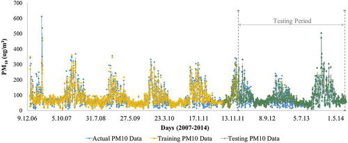
In order to depict the overall performance of NN_W1 and NN_S1 with corresponding parts of the data points used in time series data set, training and testing estimates of the models were plotted. Daily estimates obtained in training and testing were superimposed in Figure 5 on the actual data for the years 2007–2014. The higher concentrations observed in the year 2007 were followed by the model estimates, whereas the better convergences were obtained in next years. Generally, all the models estimated the data points following the historical pattern well, trying to fit peaks at elevated PM₁₀ levels. It is known that ANNs are sensitive to extreme values or outliers in the data set. However, the use of seasonal models over years resulted in better estimates comparing with singular models in this case. In the years that daily PM₁₀ levels did not fluctuate too much on daily basis, a better improvement in the estimations of seasonal ANN models may then be achieved.

Figure 5. Estimates in training and testing stage of the models NN_W1 and NN_S1 against to actual data.

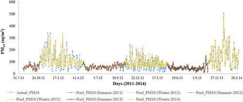
The testing results of NN_W1 and NN_S1 in seasonal sequence were plotted in Figure 6 for the period of 2011–2014. As noted before, elevated PM₁₀ levels during cold months, winter estimates (yellow points) did not overlapped with all the points completely. In contrast, estimates during summer (brown points) showed better convergences in which the fluctuations lied in a lower range than those occurred during winter. Hence, the success in the summer estimates was slightly better than the estimates for winter period.

Figure 6. Testing estimates of NN_W1 and NN_S1 models for seasons in sequence.

Time-series plots of NN_W1 and NN_S1 models’ outputs showed that daily PM₁₀ patterns have been satisfactorily followed by the related model considering convergences at peaks and valleys and statistical predictors.

It has been shown that the variable selection or determination of proper lags for the inputs of ANN models, as it is addressed in the study by Sfetsos and Vlachogiannis (2010) using an iterative process on hourly data from the days before or in the paper by Gennaro et al. (2013) that a lag-based sensitivity analysis has been applied in variable selection, could be alternatively accomplished by applying PCA. Gennaro et al. (2013) obtained R² in the range of 0.73–0.86 for daily predictions, which was better than those of singular models, whereas it was comparable to the results of seasonal models developed in this study. However, it should be noted that the results of performance measures and obtained model structures may change the approach used in modeling and the fluctuations in the data considering extremes. The obtained seasonal models demonstrated reasonable fitting performance comparing with similar studies in terms of efficiency and robustness of the applied approach.

Conclusion

The main goal of this study was to improve ANN model predictions of PM₁₀ levels 1 day ahead by applying PCA method in the selection of the most significant lagged terms of the variables as inputs, developing seasonal ANN models for winter and summer periods, and comparing singular ANN models as benchmark. The most significant lagged inputs were three consecutive lags of PM₁₀ and AT according to PCA runs. In training of ANN models, cascading-training procedure provided by FANN library was employed, which produced reasonably successful models. It may thus be an alternative way to determine the right number of hidden units in the middle layer of ANNs. For seasonal ANN models, the overall model agreement in training between modeled and observed values varied in the range of 0.78–0.83 and R² values ranged in 0.681–0.727. The best testing R² values of seasonal models for winter and summer period models ranged in 0.709–0.711, with lower testing RMSE values comparing with the nonseasonal models. Also, seasonal models did not show a tendency towards overpredicting or underpredicting the daily average PM₁₀ levels 1 day ahead with better estimates. This approach appeared to be promising in capturing nonlinear features in data and could have significant applicability in the case of the data sets with a large number of considered inputs.

ORCID

Fatih Taşpınar

http://orcid.org/0000-0002-5908-8188

Additional information

Notes on contributors

Fatih Taşpınar

Fatih Taşpınar is a professor in the Department of Environmental Engineering in the Faculty of Engineering at the University of Düzce, Düzce, Turkey.

References

- Aneja, V.P., A. Agarwal, P.A. Roelle, S.B. Phillips, Q. Tong, N. Watkins, and R. Yablonsky. 2001. Measurements and analysis of criteria pollutants in New Delhi, India. Environ. Int. 27:35–42. doi:10.1016/S0160-4120(01)00051-4
- Antanasijevic, D.Z., V.V. Pocajt, D.S. Povrenovic, M.D. Ristic, and A.A. Peric-Grujic. 2013. PM10 emission forecasting using artificial neural networks and genetic algorithm input variable optimization. Sci. Total Environ. 443:511–519. doi:10.1016/j.scitotenv.2012.10.110
- Burnett, R.T., J. Brook, T. Dann, C. Delocla, O. Philips, S. Cakmak, R. Vincent, M.S. Goldberg, and D. Krewski. 2000. Association between particulate- and gas-phase components of urban air pollution and daily mortality in eight Canadian cities. Inhal. Toxicol. 12:15–39. doi:10.1080/089583700750019495
- Chen, Y., R. Shi, S. Shu, and W. Gao. 2013. Ensemble and enhanced PM10 concentration forecast model based on stepwise regression and wavelet analysis. Atmos. Environ. 74:346–359. doi:10.1016/j.atmosenv.2013.04.002
- DMSP. 2010. Düzce Municipality Strategic Plan for 2010–2014 [in Turkish]. Düzce, Turkey: Düzce Municipality.
- FANN. 2014. Fast Artificial Neural Network library. http://leenissen.dk/fann/wp (accessed July 14, 2014).
- Gennaro, G., L. Trizio, A. Gilio, J. Pey, N. Pérez, M. Cusack, A. Alastuey, and X. Querol. 2013. Neural network model for the prediction of PM10 daily concentrations in two sites in the Western Mediterranean. Sci. Total Environ. 463–464:875–883.
- Harrison, R.M., A.R. Deacont, and M.R. Jones. 1997. Sources and processes affecting concentrations of PM10 and PM2.5 particulate matter in Birmingham (U.K.). Atmos. Environ. 31:4103–4117. doi:10.1016/S1352-2310(97)00296-3
- Henry, R.C., and G.M. Hidy. 1979. Multivariate analysis of particulate sulfate and other air quality variables by principal components—Part I. Annual data from Los Angeles and New York. Atmos. Environ. 13:1581–1596. doi:10.1016/0004-6981(79)90068-4
- Hornik, K., M. Stinchcombe, and H. White. 1989. Multilayer feed forward networks are universal approximators. Neural Netw. 2:359–366. doi:10.1016/0893-6080(89)90020-8
- Ilten, N., and A.T. Selici. 2008. Investigating the impacts of some meteorological parameters on air pollution in Balikesir, Turkey. Environ. Monit. Assess. 140:267–277. doi:10.1007/s10661-007-9865-1
- Jolliffe, I.T. 1986. Principal Component Analysis. New York: Springer-Verlag.
- Kampa, M., and E. Castanas. 2008. Human health effects of air pollution. Environ. Pollut. 151:362–367. doi:10.1016/j.envpol.2007.06.012
- Khaw, J.F.C., B.S. Lim, L.E.N. Lim. 1995. Optimal design of neural networks using the Taguchi method. Neurocomputing 7:225–245. doi:10.1016/0925-2312(94)00013-I
- Kim, Y.S., and B.J. Yum. 2004. Robust design of multilayer feed-forward neural networks: An experimental approach. Eng. Appl. Artif. Intell. 17:249–263. doi:10.1016/j.engappai.2003.12.005
- Köne, A.C., and T. Büke. 2012. A comparison for Turkish provinces’ performance of urban air pollution. Renew. Sustain. Energy Rev. 16:1300–1310. doi:10.1016/j.rser.2011.10.006
- Kurt, A., and A.B. Oktay. 2010. Forecasting air pollutant indicator levels with geographic models 3 days in advance using neural networks. Expert Syst. Appl. 37:7986–7992. doi:10.1016/j.eswa.2010.05.093
- Lu, H.C. 2002. The statistical characters of PM10 concentration in Taiwan area. Atmos. Environ. 36:491–502. doi:10.1016/S1352-2310(01)00245-X
- Madic, M.J., and M.R. Radovanovic. 2011. Optimal selection of ANN training and architectural parameters using Taguchi method: A case study. FME Trans. 39:79–86.
- Mok, K.M., and K.I. Hoi. 2005. Effects of meteorological conditions on PM10 concentrations–a study in Macau. Environ. Monit. Assess. 102:201–223. doi:10.1007/s10661-005-6022-6
- Nejadkoorki, F., and S. Baroutian. 2012. Forecasting extreme PM10 concentrations using artificial neural networks. Int. J. Environ. Res. 6:277–284.
- Nissen, S. 2007. Large scale reinforcement learning using Q-SARSA(λ) and cascading neural networks. MSc thesis, Department of Computer Science, University of Copenhagen, Copenhagen, Denmark.
- Ordieres, J.B., E.P. Vergara, R.S. Capuz, and R.E. Salazar. 2005. Neural network prediction model for fine particulate matter (PM2.5) on the US–Mexico border in El Paso (Texas) and Ciudad Juárez (Chihuahua). Environ. Model. Softw. 20:547–559. doi:10.1016/j.envsoft.2004.03.010
- Perez, P., and J. Reyes. 2002 Prediction of maximum of 24-h average of PM10 concentrations 30-h in advance in Santiago, Chile. Atmos. Environ. 36:4555–4561. doi:10.1016/S1352-2310(02)00419-3
- Sanchez-Ccoyllo, O.R., and F.M. Andrade. 2002. The influence of meteorological conditions on the behavior of pollutants concentrations in Sao Paulo, Brazil. Environ. Pollut. 116:257–263. doi:10.1016/S0269-7491(01)00129-4
- Saufie, A.Z., A.S. Yahaya, N.A. Ramli, N. Rosaida, and H.A. Hamid. 2013. Future daily PM10 concentrations prediction by combining regression models and feedforward backpropagation models with principle component analysis (PCA). Atmos. Environ. 77:621–630.
- Sfetsos, A., and D. Vlachogiannis. 2010. A new methodology development for the regulatory forecasting of PM10: Application in the Greater Athens Area, Greece. Atmos. Environ. 44:3159–3172. doi:10.1016/j.atmosenv.2010.05.028
- Statheropoulos, M., N. Vassiliadis, and A. Pappa. 1998. Principal component and canonical correlation analysis for examining air pollution and meteorological data. Atmos. Environ. 32:1087–1095. doi:10.1016/S1352-2310(97)00377-4
- Thurston, G.D., K. Ito, and R. Lall. 2011. A source apportionment of U.S. fine particulate matter air pollution. Atmos. Environ. 45:3924–3936. doi:10.1016/j.atmosenv.2011.04.070
- TURKSTAT. 2014. Online Web service of Turkish Statistical Institute (TURKSTAT). http://www.turkstat.gov.tr (accessed August 6, 2014).
- Vahlsing C., and K.R. Smith. 2012. Global review of national ambient air quality standards for PM10 and SO2 (24 h). Air Qual. Atmos. Health 5:393–399. doi:10.1007/s11869-010-0131-2