The air quality forecast rote: Recent changes and future challenges

ABSTRACT

Air quality forecasting is a recent development, with most programs initiated only in the last 20 years. During the last decade, forecast preparation procedure—the forecast rote—has changed dramatically. This paper summarizes the unique challenges posed by air quality forecasting, details the current forecast rote, and analyzes prospects for future improvements. Because air quality forecasts must diagnose and predict several pollutants and their precursors in addition to standard meteorological variables, it is, compared with weather forecasts, a higher-uncertainty forecast. Forecasters seek to contain the uncertainty by “anchoring” the forecast, using an a priori field, and then “adjusting” the forecast using additional information. The air quality a priori, or first guess, field is a blend of past, current, and near-term future observations of the pollutants of interest, on both local and regional scales, and is typically coupled with predicted air parcel trajectories. Until recently, statistical methods, based on long-term training data sets, were used to adjust the first guess. However, reductions in precursor emissions in the United States, beginning in the late 1990s and continuing to the present, eroded the stationarity assumption for the training data sets and degraded forecast skill. Beginning in the mid-2000s, output from modified numerical air quality prediction (NAQP) models, originally developed to test pollution control strategies, became available in near real time for forecast support. The current adjustment process begins with the analyses and postprocessing of individual NAQP models and their ad hoc ensembles, often in concert with new statistical techniques. The final adjustment step uses forecaster expertise to assess the impact of mesoscale features not resolved by the NAQP models. It is expected that advances in model resolution, chemical data assimilation, and the formulation of emissions fields will improve mesoscale predictions by NAQP models and drive future changes in the forecast rote.

Implications: Routine air quality forecasts are now issued for nearly all the major U.S. metropolitan areas. Methods of forecast preparation—the forecast rote—have changed significantly in the last decade. Numerical air quality models have matured and are now an indispensable part of the forecasting process. All forecasting methods, particularly statistically based models, must be continually calibrated to account for ongoing local- and regional-scale emission reductions.

Introduction

Rote is defined as a routine or habitual course of procedure. In weather forecasting, rote refers to the set of task structures used in preparing a forecast. The rote includes both diagnostic and prognostic tools and acts as an information filter to enhance the efficiency of time-constrained operational forecasts (Doswell, 2004). This paper summarizes a version of the current forecast rote for air quality forecasting and, using illustrations from operational forecasts, provides insight into air quality forecast preparation and the tools used by forecasters. Real-time air quality forecasting (RT-AQF) began in the United States (U.S.) in the 1970s in southern California and New York. Beginning in the mid-1990s, air quality forecasts became common in major metropolitan areas of the eastern U.S. (Ryan et al., 2000). For a complete review of air quality forecasting history, the reader is directed to Zhang et al. (2012a) and Zhang et al. (2012b). A brief synopsis is included in this introduction. The first generation of air quality forecasts focused on next-day peak 1-hr mixing ratios of ozone (O₃). Although technically O₃ is measured as a mixing ratio (in parts per billion by volume, ppbv), in practice O₃ mixing ratios are often referred to as a “concentration.” The current health standard in the U.S., the National Ambient Air Quality Standard (NAAQS), for O₃ is based on longer-term average concentrations—an 8-hr average. Following a series of health studies, the NAAQS for fine particulate matter (aerodynamic diameter <2.5 μm; PM_2.5) was tightened and next-day forecasts of PM_2.5 were added in the early 2000s. Today, hundreds of states and municipalities provide daily air quality forecasts for O₃ and PM_2.5 along with other pollutants (U.S. Environmental Protection Agency [EPA], 2015). In Europe, daily forecasts of nitrogen dioxide (NO₂) are routinely provided and, based on changes to the NAAQS for NO₂, forecasts for NO₂ may become common in the U.S. (EPA, 2010).

The early air quality forecasts for O₃ relied on empirical approaches, primarily statistical models, trained on historical air quality and meteorological data—the so-called “perfect prog” approach (Klein, 1971). These methods included multiple linear regression (Robeson and Steyn, 1989; Ryan, 1995; Ryan et al., 2000), nonlinear regression (Cobourn et al., 2000), neural networks (Ruiz-Suárez et al., 1995; Comrie, 1997), and Classification and Regression Trees (CART) (Burrows et al., 1995). Regardless of the technique, all statistical methods relied on the close association of O₃ with a small set of meteorological and chemical predictors. The most commonly used predictors were maximum surface temperature (T_max), persistence (previous day) O₃, wind speed, near the surface and aloft, cloud cover, and a seasonal cycle variable (e.g., Julian date, solar zenith angle). Emissions of O₃ precursors were assumed to be constant day to day, although a separate algorithm for weekend days could be constructed. The training data sets typically used 5–10 years of historical observations. Because O₃ is a photochemical pollutant, the training data were restricted to warm season days (May–September) so that the total number of cases used to develop, train, and test the statistical forecast models was on the order of ~10²–10³. The forecast rote during this period consisted of collecting the appropriate input data for the forecast day and applying the model. The statistical guidance was then used as a first guess for “expert” analysis leading to the final forecast. Statistical approaches proved reasonably accurate throughout the 1990s and early 2000s (Comrie, 1997; Ryan et al., 2000).

The current forecast rote is significantly changed from the early days of air quality forecasting. A comprehensive review of forecast tools used through the 1990s can be found in EPA (2003). These changes occurred gradually through the early 2000s and were driven by several factors, of which three are highlighted here. First, pollution control efforts, primarily electric generating unit (EGU) nitrogen oxide (NO_x) controls and the introduction of cleaner cars, significantly reduced O₃ precursor emissions (He et al., 2013). This led to a large decrease in O₃ concentrations (Gilliland et al., 2008; Godowitch et al., 2008a, 2008b, 2010), particularly in the eastern U.S. (Butler et al., 2011; Cooper et al., 2012). In particular, after the EPA issued the NO_x State Implementation Plan (SIP) Rule, also known as the “NO_x SIP Call” in 1998, with implementation phased in over the next several years, statistical models began to lose skill. The decline in O₃ precursor emissions meant that the statistical model training data set no longer accurately represented current conditions. This led the statistical models to overpredict O₃, particularly in the upper end of the O₃ distribution. In Figure 1, forecast biases for two operational statistical O₃ forecast models developed and used by the author for operational forecasting in Philadelphia are given. Both models used multiple linear regression techniques, although the sets of predictors and training data sets varied. The seasonal bias increased roughly 5 times over the period 2003–2009. Simultaneously, advances in computational efficiency and optimization practices allowed numerical air quality prediction (NAQP) models to be used for operational forecast guidance. In the 1990s, chemical-transport models (CTM) were used for the simulation of historical poor air quality episodes in order to test the efficacy of proposed pollution control strategies. In the regulatory setting, unlike operational forecasting, processing speed was not a concern. With improvements in computation speed, optimization of emissions preprocessing, and improvements in chemical mechanisms and meteorological parameterizations, real-time NAQP models began to be used as forecast guidance (McHenry et al., 2004; Zhang et al., 2012a, 2012b). The use of NAQP model guidance in air quality forecast operations became widespread in the U.S. following the development and deployment of the National Air Quality Forecast Capability (NAQFC) model in the mid-2000s (Otte el al., 2005; Eder et al., 2006, 2009; Yu et al., 2007; McKeen et al., 2009; Doraiswamy et al., 2010). The final factor that increased the use of NAQP models in the forecast rote was the growing awareness of the health dangers posed by PM_2.5 and the subsequent revisions to its NAAQS. This led many state and local air quality protection agencies to extend air quality forecasts to include PM_2.5. Unlike O₃, which is produced primarily by gaseous and photochemical reactions, PM_2.5 is emitted directly and is also formed via a wide variety of mechanisms, including aqueous- and solid-phase processes. As a result, statistical forecast approaches for PM_2.5, based on meteorological and chemical predictors in a manner similar to O₃ forecasts, were never very skillful. In addition, because PM_2.5 and O₃ share common precursors (NO_x, volatile organic compounds [VOCs]), PM_2.5 training data sets also suffer from the same secular changes in emissions that degraded O₃ statistical models. The absence of another adequate prognostic technique made numerical model guidance a necessary tool for PM_2.5 forecasts (Yu et al., 2008).

Figure 1. Forecast bias for two operational O₃ statistical forecast models (REG1 and REG2) used in the Philadelphia Forecast Area (PHLFA) for the period May–September 2003–2009. REG1 and REG2 both used multiple linear regression methods but varied with respect to predictor selection and training data sets. The forecast metric is domain peak 8-hr O₃ mixing ratio.

The air quality forecast

Worldwide, health forecasts are issued for a number of airborne pollutants. The most common forecast pollutants are carbon monoxide (CO), fine particles with aerodynamic diameter less than 10 μm (PM₁₀) or less than 2.5 μm (PM_2.5), ozone (O₃), and nitrogen dioxide (NO₂). This paper will focus on the forecast rote for PM_2.5 and O₃, although the techniques discussed here are applicable to other pollutants. The standard forecast verification metric for air quality forecasts is domain-wide peak concentration (or mixing ratio) of the pollutant of interest or of a group of pollutants. The averaging period varies by pollutant and jurisdiction. In the U.S., peak O₃ is determined by an 8-hr average at an individual monitor and PM_2.5 by a 24-hr (midnight to midnight) average. The Canadian Air Quality Health Index (AQHI) uses a 6-hr average of a weighted suite of pollutants (Taylor, 2014). The forecast is typically released to the public with reference to a set of nondimensional thresholds (in the U.S., the Air Quality Index or AQI) ranging from “good” to “hazardous” and often connected to color codes for ease of understanding. Health warnings are issued for forecasts above a given threshold. In the U.S., for example, the current health threshold for O₃ is ≥76 ppbv (8-hr average) and for PM_2.5 ≥35.5 μg m⁻³ (24-hr average). The public health warnings that follow forecasts in excess of the threshold (often called “Code Orange” or “Code Red,” and for more extreme cases, “Code Purple” plus “Code Maroon” for hazardous situations) identify the “at-risk” population (e.g., very young, very old, anyone with compromised respiratory or cardiopulmonary systems) and suggest actions that the public can take to protect itself. These forecasts are widely used by the health care community to reduce exposure to poor air quality (Wen et al., 2009; Casio et al., 2013). On October 25, 2015, the NAAQS for O₃ was strengthened to 70 ppbv (EPA, 2015a). This rule will become effective on December 28, 2015, and will result in changes to the forecast thresholds noted above. This will increase the need for improvements in the forecast rote as category ranges shrink.

In addition to the dissemination of public warnings, many metropolitan areas have developed public and private initiatives (often called “Action Day Programs”; see, for example, Triangle Air Awareness, 2015) that are activated on forecast. As part of these programs, private and public employers may suspend certain high-emissions industrial operations or allow liberal leave on forecast Action Days. This aspect of air quality forecasting, where forecasts can engage efforts to curb emissions and influence the predictand itself, is unique to air quality forecasting. The time required to activate Action Day plans places constraints on the forecast timing and its latency period. In most locations, the air quality forecast must be issued in the late morning or early afternoon (11:00 am–3:00 pm in the eastern U.S.)in order to allow sufficient time for Action Day partners to be alerted and for their programs to be put into effect. The air quality forecast is therefore a 12–36-hr forecast. At this time scale, the forecast will be subject to influences on both the synoptic scale and mesoscale. This forecast latency period has important implications for forecast preparation and the use of numerical forecast models, as will be detailed below.

The focus of the air quality forecast rote follows from the key parameters that regulate the production of O₃ and PM_2.5. These parameters include the current state of the chemical atmosphere and include concentrations of the forecast pollutants and their precursors. In addition, the transport of pollutants and precursors into and out of the domain over the forecast period must be accounted for as well as the expected local and regional emissions of precursors. The transport question requires a prediction of the path of an air parcel throughout the depth of the lower troposphere. Because air quality is measured near ground level using a volume metric, the depth and rate of change of the planetary boundary layer (PBL) into which the pollutants and their precursors are mixed becomes of great importance. The amount of short-wave radiation, which depends on season and amount of cloud cover, controls photochemical reactions both locally and along the presumed transport path. The amount and location of moist layers are important not only for photochemical effects but also regulating the production of PM_2.5, including both sulfur oxide (SO_x)- and NO_x-based particles. Convection and precipitation, including its timing and extent, has a strong effect on O₃ but can also modulate PM_2.5 as well. As is immediately obvious, many of these key forecast parameters (transport, cloud formation, PBL development, convection) are extremely difficult to forecast and the resolution required is typically beyond the requirements of a standard weather forecast model. As a result, the air quality forecast resides in a large uncertainty space. The air quality forecast rote, detailed below, represents a method to adjust to these uncertainties.

The forecast rote with operational examples

Background

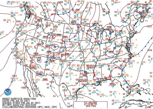
In order to better understand the forecast rote, this section will move sequentially through the forecast preparation process, explaining each component in turn, and use examples when necessary from an extended poor air quality event during early July 2011 in the Mid-Atlantic region of the U.S. During that period, PM_2.5 and O₃ concentrations in excess of the Code Orange (warning) threshold occurred intermittently over an area stretching from Massachusetts to North Carolina and extending west to Ohio. The forecast area of interest for this discussion is the EPA-designated Philadelphia-Wilmington-Atlantic City nonattainment area. This area includes portions of southern New Jersey and northern Delaware as well as the city of Philadelphia and its adjacent counties. For ease of reference, and to avoid confusion, we will refer to the forecast domain as the Philadelphia metropolitan forecast area (PHLFA). A complete case study, with detailed discussion, can be found at Ryan (2011). For our period of interest, July 1–3, O₃ was the leading pollutant, with peaks centered along the I-95 Corridor. PM_2.5 concentrations were higher than average but remained in the range of 10–25 μg m⁻³. The synoptic pattern associated with the onset of this event was standard for poor air quality events in this region (Ryan et al., 1998). A 500 mb ridge, with its axis west of the Mid-Atlantic, assured subsidence and stable conditions aloft (Figure 2). At 850 mb, near the top of the afternoon PBL or what is often termed the “transport layer,” the semipermanent summer season Bermuda High had extended (retrograded) to the west (Figure 3). This alignment drives down sloping westerly flow in the lee of the Appalachians and enhances low-level stability. In addition, westerly flow transports air from the Ohio River Valley, rich in O₃ and PM_2.5 precursors, into the Mid-Atlantic. Surface high pressure leads the mid-level ridge axis and is centered over the Mid-Atlantic, resulting in light winds (Figure 4).

Figure 2. Mean geopotential height (m), using 20th century reanalysis version 2 data, for the period July 1–3, 2011. Figure courtesy of NOAA ESRL.

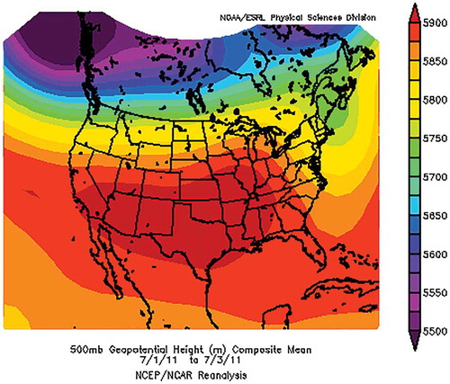
Figure 3. As in Figure 2, but for 850 mb geopotential height (m).

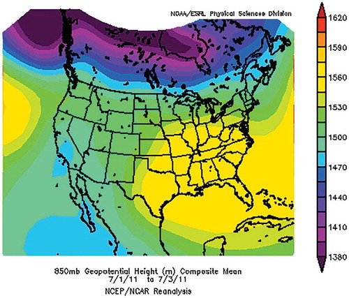
Figure 4. Surface weather analysis for 12:00 a.m. UTC, July 1, 2011.

Use of persistence with local and transport adjustments

As previously noted, air quality forecasts must account for both meteorological and chemical phenomena, and their interactions, and are characterized by high uncertainty. As a result, the forecast rote follows a variation on the “anchoring and adjustment” technique (Doswell, 2004). This can be thought of as a “poor man’s” Bayesian approach in which the initial forecast, also termed the a priori or first guess, is bounded (“anchored”) within some reasonable range, and then “adjusted” to reflect additional information from other forecast guidance sources. The main anchor in the air quality forecast rote is persistence—today’s concentrations used as the forecast for tomorrow. Both O₃ and PM_2.5 have relatively long lifetimes in the lower troposphere (on the order of days), as do some of their precursors. This phenomenon makes persistence a useful anchoring forecast. Climatology may be useful in quantifying the expected range of the forecast with respect to time of year, and can bound the magnitude of extreme cases, but is of limited use otherwise. For example, mean peak O₃ concentrations, averaged over a number of years, in the PHLFA are relatively steady for the period June 15–August 15, although day-to-day variations during this period are on the order of 10s of ppbv. In addition, climatology is a poor predictor in situations such as the eastern U.S. where pollution controls and changes in fuel use (“fuel switching”) as well as retirement of coal fired plants have resulted in a significant decade-long downward trend in precursor emissions and pollutant concentrations (Butler et al., 2011; Cooper et al., 2012). In the absence of stationarity, therefore, climatology for O₃ and PM_2.5 cannot be relied upon for forecasting purposes.

Persistence can be approximated in a number of ways. “Local” persistence draws on observations from the nearby monitor network. The air quality observation network for the PHLFA, for example, draws from 10–20 O₃ monitors and 5–10 continuous PM_2.5 monitors. These monitors are irregularly dispersed in space, with highest density near the urban center. Although O₃ and PM_2.5 observations are reasonably dense, those of their key precursors are very limited. For example, measurements of oxides of nitrogen (NO_x), an important precursor for both O₃ and PM_2.5, are few and are typically located near high motor vehicle traffic areas in order to measure peak concentrations of NO₂—itself a criteria pollutant for which a NAAQS exists. These locations are not representative of metropolitan-scale concentrations. Hydrocarbon measurements (VOCs) are technically complex and require laboratory analysis, resulting in a long latency period that makes them not useful for operational forecasting.

Although the observation network of O₃ and PM_2.5 monitors are sufficiently dense for operational purposes, they must be adjusted for the timing of the forecast. Forecasts are typically issued in the early afternoon. Persistence, defined as the current day peak concentration, is not fully known until much later in the day, so a short-range (0–10-hr) forecast is required to accurately approximate current day peak concentrations. In training data sets, where peak concentrations are known, local persistence is a useful predictor for both PM_2.5 and O₃. For the summer season in the PHLFA, for example, the correlation for both PM_2.5 and O₃ persistence and their next-day peaks are in the range of 0.5–0.6, although PM_2.5 persistence becomes less useful in the cool season (Figure 5). Because short-range persistence forecasts are not error free, the correlation in operational use is likely somewhat lower. For the initial forecast day of our example case (July 1), persistence in the PHL area (June 30) for O₃ was ~60 ppbv. Higher O₃ concentrations, in the range of ~70 ppbv, were observed just south of the Mason-Dixon Line. PM_2.5 concentrations were low (8–10 μg m⁻³) along the I-95 Corridor, suggesting that the air mass on June 30 was relatively unmodified. Because O₃ and PM_2.5 share a number of precursors (NO_x, VOCs), they tend to be tightly correlated. An analysis by the author of the correlation coefficient between peak O₃ and PM_2.5 in the PHLFA during this time period (2010–2012) in the PHLFA was 0.75.

Figure 5. Scatterplot of previous day (persistence) domain peak 8-hr O₃ in the PHLFA (x-axis) and current day (y-axis) for the period June–August 2004–2014. Correlation coefficient (r) = 0.54, r² = 0.29, linear best fit line given as: [O₃]_obs = 29.0 + 0.54·[O₃]_persistence.

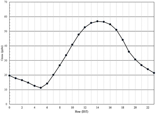
In nearly every case, however, the air mass overhead today is not expected to remain there tomorrow. Local persistence is a truly accurate forecast measure only in extreme stagnation events. As a result, local persistence must be adjusted by some measure of regional or “transport” persistence. The standard method for determining transport persistence, or the current day characteristics of tomorrow’s incoming air mass, is to combine back trajectory model output with current upwind surface observations. The adjustment is usually done qualitatively but can also be developed within a statistical forecast algorithm (Cobourn and Hubbard, 1999; Cobourn, 2007). Back trajectory forecasts for operational air quality forecasting have traditionally used the National Oceanic and Atmospheric Administration Air Resources Laboratory (NOAA-ARL) HYSPLIT (Hybrid Single-Particle Lagrangian Integrated Trajectory) semi-Lagrangian system (Draxler and Hess, 1998; Draxler and Rolph, 2015). In the simplest terms, back trajectories forecast the track of a hypothetical air parcel prior to its arrival over a selected location. Figures 6 and 7 are two examples of the use of back trajectories in operational forecasting. The duration of the back trajectory in these cases is 24 hr beginning at 12:00 p.m. UTC on the day of the forecast and moving backwards in time. In order to reduce the impact of low-level turbulence, and O₃ losses due to NO_x titration and dry deposition within the nocturnal stable layer, back trajectories are usually initiated well above the surface and within the expected overnight residual layer (~500–1500 m above ground level [AGL]). HYSPLIT accommodates a variety of operational numerical weather prediction (NWP) models in order to drive the trajectory forecast. For the July 1 forecast, the back trajectories shown in Figure 6 used the operational North American Model (NAM) model as input to the HYSPLIT model. The back trajectory terminating at PHL on July 1 originated on the previous day in southern Quebec. A back trajectory calculated after the fact using NAM analysis fields (not shown) was very similar to the forecast trajectory with respect to both source region and track. By way of reference, an analysis back trajectory for the Richmond, Virginia (RIC), area is shown in Figure 7. In the RIC case, the source region is located well to the southwest of the PHL back trajectory and suggests a source region in northern Ohio. The back trajectory data are then coupled with current observed data via the EPA AirNow network (EPA, 2015b). There are a variety of methods to quantitatively couple trajectory forecasts and current observations. Due to the strong diurnal gradient in surface O₃ concentrations (Figure 8)—PM_2.5 also has diurnal gradients but these are significantly lower in magnitude—only surface observations after 3:00 p.m. UTC, when the boundary layer is presumed to be well mixed, are reflective of persistence concentrations. The source region for air parcels expected to arrive in the residual layer over PHL on July 1 included Rochester and western New York as well as Scranton-Wilkes-Barre, Pennsylvania. As of 5:00 p.m. UTC on June 30, hourly O₃ concentrations in those locations had a range of 29–42 ppbv. The source region for air parcels expected to arrive in the residual layer over RIC on July 1 included the Cleveland and Pittsburgh metropolitan areas. As of 5:00 p.m. UTC on June 30, hourly O₃ concentrations in those locations had a range of 51–65 ppbv. As is the case with local persistence, a correction factor, based on climatology, can be developed to adjust 1-hr O₃ observed at 5:00 p.m. UTC to peak concentration that occurs later in the day. This correction factor (k) likely varies by region. For the PHFLA, based on observations on days with peak 1-hr O₃ in the moderate range (60 ppbv) or higher, from 2003 to 2014, the 1-hr peak concentration can be approximated by multiplying hourly O₃ at 5:00 p.m. UTC by k ~ 1.2. This empirical correction proved to be adequate in this case, as peak concentrations observed in Pittsburgh and Cleveland (79 and 75, respectively) were forecast to be 78 and 76 ppbv. For Rochester and Wilkes-Barre, the observed peaks, 57 and 44 ppbv, were estimated at 50 and 49 ppbv. The O₃ concentrations observed along the two forecast paths therefore varied by roughly 20–30 ppbv, with the RIC back trajectory carrying higher O₃ air.

Figure 6. 24-hour NOAA ARL HYSPLIT back trajectories for 12:00 p.m. UTC, July 1, 2011, at PHL terminating at 500, 1000, and 1500 m above ground level (AGL). The back trajectories were calculated using the June 30, 6:00 a.m. UTC operational NAM.

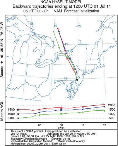
Figure 7. As in Figure 6 except terminating at RIC and using meteorological data from NAM analysis fields.

Figure 8. Average hourly O₃ mixing ratios at the Pennsylvania Department of Environmental Protection (PADEP) Bristol, Pennsylvania, monitor for all days with maximum surface temperature at PHL ≥80 °F for the period June–August 2010–2012.

An alternative approach to determining transport persistence via surface O₃ observations is to seek out observations at locations that have little diurnal variance in O₃. These monitors are located at high elevation, usually in rural surroundings, and are often referred to as “sentinel” monitors. In the Mid-Atlantic, there are a number of these monitors, primarily situated along the spine of the Appalachians. For our example, monitors at Methodist Hill, Pennsylvania (750 m above sea level [ASL]; 39.96°N, 77.48°W), and Shenandoah National Park, Virginia (1000 m ASL; 38.54°N, 78.43°W), are located within the trajectory path for PHL and RIC, respectively. O₃ concentrations from these monitors for June 29–30 are shown in Figure 9. Based on observations from these “sentinel” monitors, residual layer O₃ over the PHLFA on the morning of July 1 is expected to be ~45 ppbv, whereas further south at RIC, concentrations are expected to be significantly higher—on the order of 70 ppbv. Because the diurnal range of O₃ is small at high elevation sites, little adjustment is required to reflect later day peak concentrations. The results of the various persistence measures, and other forecast guidance information for July 1, are given in Table 1.

Table 1. O₃ forecast guidance for July 1, 2011 (all measures in ppbv).

Parameter	PHL	RIC
Adjusted local persistence	62	70
Adjusted transport persistence	48	74
Sentinel monitor average	54	84
NAQFC	65	76
Ensemble of NAQP models	67	75
Range of AQNM models	[62, 72]	[69, 79]
Forecast	68	72
Observed	67	83

Notes: Adjusted local and transport persistence values represent short-term forecasts of peak 8-hr O₃ using observations up to 5:00 p.m. UTC as a base value. Sentinel monitors are high-elevation O₃ monitors in rural locations upwind of the forecast area. In this example, they include Shenandoah National Park (Big Meadows), Virginia, and Methodist Hill, Pennsylvania. NAQFC refers to the operational NOAA Numerical Air Quality Forecast Model. The ensemble of NAQC models includes the NOAA model as well as model output provided by Baron Meteorological Services and the State of North Carolina.

Figure 9. Hourly O₃ concentrations for monitors at Methodist Hill, Pennsylvania, and Shenandoah National Park, Virginia, for the period from 12:00 a.m. EST (05:00 a.m. UTC) June 29, 2011, to 2:00 p.m. EST (7:00 p.m. UTC) June 30, 2011. Location and elevation of monitors given in the text.

Use of numerical air quality prediction models

As noted above, NAQP models are now a critical source of forecast guidance and are the primary step in the adjustment process. A list of NAQP models used regularly in the Mid-Atlantic is given in Table 2. A more detailed description of these models as well as other numerical models used worldwide can be found in Zhang et al. (2012b). NAQP models as used in the eastern U.S. are typically run two to four times daily, with 6:00 a.m. and 12:00 p.m. UTC runs common to all models. In nearly all cases, the NAQP models use the prior (6-hr) run to initialize the succeeding run. In the eastern U.S., air quality forecasters rely on the 6:00 a.m. and 12:00 p.m. UTC model runs for operational guidance. Due to the higher computational requirements for a coupled CTM, the 12:00 p.m. UTC air quality guidance reaches the forecasters well after the 12:00 p.m. UTC NWP model output and, in some cases, immediately prior to the afternoon forecast deadline.

Table 2. Selection of links for Mid-Atlantic numerical air quality forecast model guidance.

Model	Link
NAQFC (NOAA)	http://www.emc.ncep.noaa.gov/mmb/aq/
Baron AMS	https://products.baronams.com/clients/usfs_models.html
North Carolina DENR	http://staging.daq.state.nc.us/airaware/forecast/model/
GEM-MACH (Canada)	http://weather.gc.ca/aqfm/index_e.html
WRF-Chem	http://ruc.noaa.gov/wrf/WG11_RT/
North Carolina State University	http://www.meas.ncsu.edu/aqforecasting/Real_Time.html

NAQP models address a more challenging problem than operational NWP models. Although both types of models solve the standard set of “primitive” equations using numerical methods and parameterizations, NAQP models must also diagnose and predict a wider range of variables, including trace gases and aerosols along with the interactions between them. This includes accurate determinations of the sources and sinks of reactive gases as well as liquid- and solid-phase particles. Simply addressing the issue of many more predictands increases the computational effort required. In addition, the air quality problem places more acute stress on certain model components than standard NWP applications. The chemical species of interest for NAQP models have extremely variable lifetimes in the troposphere. As a result, the chemistry model, in order to handle both very fast and relatively slow reactions, is faced with a numerically “stiff” problem. Solution techniques for this situation can be computationally very expensive and sensitive to the update time between the meteorological and chemistry models. Short chemical lifetimes also result in large concentration gradients in both the horizontal and vertical, which place a higher burden on the accuracy of modeled advection and diffusion terms. Finally, the health effects of poor air quality are primarily a PBL phenomenon. As a result, NAQP models are more sensitive to errors in turbulent processes and to the parameterization methods that are used to close the turbulence equations and determine the state of the boundary layer.

Even assuming a perfect weather forecast from the NWP model, its output may be degraded when incorporated into the chemistry model. NAQP models come in two flavors: “offline” and “online”—the latter sometimes referred to “inline” (Grell et al., 2005; Zhang, 2008; Grell and Baklanov, 2011; Im et al., 2015). Offline describes an air quality modeling system where meteorology is simulated independently of chemistry. Output from the meteorology model, often termed the “driver,” is passed, at prescribed time steps, to the air quality model using an interface that interpolates the state variables from the NWP to the NAQP model grids (e.g., Otte and Pleim, 2010). The amount of interpolation required is a function of the degree of “coupling” or consistency between the two models. A weakly coupled set of offline models will vary with respect to horizontal grid spacing and staggering, map projection, vertical coordinates, and number of layers, as well as the length of discrete time steps between the two models. Although offline NAQP models are computationally less expensive, interpolation inexorably results in the loss of information at each step (Pielke and Uliasz, 1998). This is particularly true for atmospheric processes that have a time scale less than the time scale at which meteorological information is passed. By way of example, the operational NAQP models used by forecasters for the July 2011 case are all offline models. For example, the operational NAM, then a version of the Non-hydrostatic Mesoscale Model (NMM) in the Weather Research and Forecasting (WRF) model framework (Janjic, 2003; Rogers et al., 2006), provided the meteorological driver that was used by the Community Multi-Scale Air Quality (CMAQ) model in the NAQFC-coupled model during 2011 (Byun and Schere, 2006; Otte et al., 2005; Appel et al., 2012). Since that time, the NAQFC has moved to tighter coupling of the NAM and the CMAQ (National Center for Environmental Prediction [NCEP], 2015; Lee et al., 2012) and the operational use of online models has expanded (Kukkonen et al., 2012; Im et al., 2015). Online models solve both meteorological and chemistry variables on the same native grid. In addition to avoiding interpolation issues, the inline model structure can allow for two-way feedback between the models. For example, aerosol formation driven by the chemistry model can influence radiation and temperature in the meteorological model. The drawback of the inline model is the larger computational overhead that is required. As computing resources continue to increase, the trend toward inline models will continue.

Beyond errors related to the coupling of meteorological and chemical models, NAQP models are also subject to errors from sources that are usually less problematic in the NWP model setting. Most NWP models were originally designed to focus on situations of strong dynamical forcing and deep convection. Most poor air quality events occur in weakly forced dynamical conditions where physical parameterization schemes become of more importance (Seaman, 2000). NWP models, in addition to solving the dynamical equations, must account for forcing from initial conditions, radiation, and friction. Significant attention in both research and operations has been paid to addressing these issues by improving data assimilation and initialization techniques as well as radiation, microphysical, and turbulence parameterization schemes. NAQP models must account for those forcings, but they are also sensitive to a number of other factors, including, inter alia, boundary conditions, PBL development, emissions of pollutant precursors, and the effect of unusual weather events such as wildfires and dust storms. Because operational NAQP models are limited area models (LAMs) run for up to five simulation days, they become increasingly sensitive, depending on the size of the model domain, to boundary conditions (McKeen et al., 2005; Chuang et al., 2011). As noted above, an accurate simulation of PBL development is essential to predicting pollutant concentrations but, except for convective parameterization triggers, it is less important in NWP models (Vautard et al., 2012). Emissions drive the chemical processes and vary in scale from large emitters in small areas, termed point source emissions (e.g., electric generating units [EGUs]), to small emitters spread over large areas, termed area source emissions (e.g., dry cleaners, gas stations). Area source emissions include natural (biogenic) hydrocarbons emitted by plants and trees, as well as emissions from on-road and off-road vehicles. The rate of these emissions varies in response to ambient weather conditions. For example, biogenic hydrocarbon emissions are sensitive to temperature, whereas motor vehicle emissions are sensitive to both temperature and local driving conditions and fleet makeup. There can also be secular changes, on daily to annual scales, due to variations in the operation of large emitters, improvements in pollution control technologies, and changes in energy use. Statistical forecast methods do not explicitly treat emission variations and, instead, assume constant background emissions throughout the training period. Operational numerical models, in an effort to streamline computing resources, typically use yearly updated weekday and weekend emissions fields and allow limited emission variations related to meteorological effects. Uncertainties in the emissions fields, and their effect on model performance, are difficult to quantify but are expected to be the most significant source of model error (Hanna et al., 2001).

As a result, users of NAQP model guidance must adjust for errors in the meteorological simulation, errors in interpolation from the meteorological driver to the chemistry model, errors in boundary conditions and emission estimates, and errors in the simulation and parameterization of chemical interactions. Compounding the situation in the operational setting is the timeliness requirement that requires simplified and optimized options for dynamics, physical parameterizations, and chemistry in order to meet forecast deadlines (McHenry et al., 1999).

In the Mid-Atlantic region, NAQP model guidance for O₃ has shown adequate overall accuracy (Garner, 2013; Garner and Thompson, 2012). Recent results for the NAQFC model in the PHLFA are given in Figure 10. In other regions and locations, errors characteristics can be much different (Pan et al., 2014). The forecast rote provides methods to adjust to model uncertainty issues in several ways. Because O₃ and PM_2.5 have relatively long lifetimes in the troposphere, they respond to synoptic-scale weather phenomena. With this in mind, a simple short-term (on the order of days) bias correction can be a useful adjustment method (McKeen et al., 2005; Wilczak, 2006; Djalalova et al., 2010). Its weakness, of course, is during periods of transition between synoptic cycles. Simple bias correction has not been useful in the PHLFA. For the time period bracketing our example case (2010–2012), the use of a 1-day or 2-day lagged bias correction for O₃ resulted in a degradation of mean absolute error ranging from 11% to 29% depending on the subset of cases selected. As will be noted below, more sophisticated bias correction methods do hold promise. In the PHLFA, a seasonal-scale bias correction measure has been useful. For example, applying a seasonal bias correction based on summer season (JJA) 2011–2012 NAQFC forecast guidance for the PHLFA in 2013, median absolute error improved by 16%. Unfortunately, the bulk of this improvement is due to cases in the lower end of the O₃ distribution (≤60 ppbv). For warm cases (T_max ≥80 °F) with peak O₃ concentrations ≥60 ppbv, seasonal bias corrected forecasts are less accurate (median absolute error increases from 5.9 to 7.5 ppbv). In the operational forecasts for July 1–3, 2011, where forecast T_max ≥85 °F, and local persistence expected to be ≥60 ppbv, no bias correction was applied. Another adjustment method addresses a NAQP model artifact often termed “seasonal drift.” In Figure 11, NAQFC daily forecast bias is averaged over the 2007–2013 summer O₃ seasons. The NAQFC model is generally unbiased for the first portion of the summer and then an overprediction bias gradually increases throughout the remainder of the season. This drift is observed in other NAQAP models for this region. The reasons for the seasonal drift remain unclear. A seasonal drift bias correction measure based on 2007–2013 data was applied to 2014 forecasts and resulted in a ~0.5 ppbv decrease in mean and median absolute errors, representing an 8% improvement in this skill measure. In any event, in our example case in very early July, the assumption is that the seasonal drift will not be a factor.

Figure 10. Median absolute error for the PHL metropolitan area “expert” forecast (Forecast) and for the NOAA National Air Quality Forecast Capability model guidance (NAQFC) for the period May–September 2008–2014. The forecast metric is domain peak 8-hr O₃ mixing ratio.

Figure 11. Average daily forecast bias (columns) for the NAQFC model and 7-day running average bias (line) for the period May 1–September 15, 2007–2013.

Although the NAQFC model is the most commonly used model by forecasters in the U.S., there are a number of operational models available to the forecaster community. A sampling of NAQF models that have been reliably available for operational forecasters in the eastern U.S. as of 2015 is given in Table 2. For the Mid-Atlantic region in 2011, the North Carolina Department of Environmental and Natural Resources, Baron, and NAQFC models were commonly used. They are all offline models with different meteorological drivers, parameterization schemes, emissions fields, and similar, though not identical, versions of the CMAQ chemistry model. As a result, they can be combined in ad hoc multimodel ensembles and provide a reasonable distribution of predictions, although certainly far short of a robust sample of probabilities. In addition, the expected skill of the ensemble forecast for any given year is difficult to assess. All the NAQP models change year to year due to upgrades in the meteorological and chemistry models and their associated parameterizations, as well as the emissions fields. This makes a more sophisticated weighted ensemble system based on bias and skill performance measures over time problematic.

In the PHLFA, a simple weighted average of these three models is used to prepare a consensus guidance value. Results for the ensemble forecast as applied in the 2013–2014 O₃ forecast season are given in Figure 12. The NAQFC model was the most skillful single model for this period and is used to quantify the skill added by the ensemble. For the first day of our example forecast, July 1, the range of NAQP model guidance and the ensemble weighted average for the PHLFA are given in Table 1. Applying the forecast rote process outlined above to the PHL forecast area, local and regional O₃ concentrations, constituting the first guess forecast, are in the range of 48–62 ppbv. The numerical forecast guidance are higher, with a range of 65–72 ppbv, and an ensemble average of 67 ppbv. For the RIC forecast area, the first guess forecast based on current observations and transport suggests much higher concentrations, in the range of 70–84 ppbv. The numerical forecast model guidance ranges from 69 to 79 ppbv, with an ensemble forecast of 75 ppbv—just at the Code Orange warning threshold.

Figure 12. Forecast skill measures (bias, mean absolute error, and median absolute error) for the NAQFC and the ensemble of numerical air quality forecast models (ENSEM) for 2014.

Heuristics and expert adjustment

Both statistical and numerical model guidance tend to encounter problems in the higher end of the O₃ distribution, particularly at and above the warning threshold for O₃ (Code Orange AQI, or ≥76 ppbv). Statistical models, particularly those constructed using regression techniques, tend to perform best near the mean and are less successful at the extremes of the distribution. As a result, operational use of statistical model guidance is limited to acting as a “sanity check.” Numerical models are expected to perform better at the upper range of the pollutant distribution, but only if they have sufficient resolution to address the key phenomenon driving a specific forecast scenario. Periods of regional-scale poor air quality are associated with synoptically quiescent conditions, featuring upper-level ridges and enhanced surface pressure. These conditions can be resolved by current NWP and NAQP models but are also conducive to the development of mesoscale circulations that are otherwise inhibited in stronger-forced situations. In coastal areas like the PHLFA, weakly forced synoptic conditions allow the development of bay and sea breezes (Stauffer et al., 2012; Stauffer and Thompson, 2013). Current operational NAQP models, generally at 12 km horizontal grid resolution, cannot fully resolve the location and strength of land-water circulations or the chemical interactions when these circulations intersect with gradients in emissions (Loughner et al., 2011, 2014). Other mesoscale phenomena specific to the Mid-Atlantic region include Appalachian lee side troughs (Weisman, 1990). These troughs are associated with high O₃ and PM_2.5 concentrations and feature large concentration gradients normal to the trough axis, with highest concentrations to the east (Pagnotti, 1987; Gaza, 1998; Seaman and Michelson, 2000). Because the lee side trough is rarely stationary throughout the day, and is usually aligned parallel to the high-emissions I-95 Corridor, resolving the location and movement of the trough axis is a critical air quality forecast question. In addition, nocturnal low-level jets (LLJs) are frequently observed in quiescent synoptic weather and during poor air quality events (Zhang et al., 2006; Hu et al., 2013). Whereas upper-level (≥1 km AGL) transport is often west to east in regional poor air quality episodes in the Mid-Atlantic (Ryan et al., 1998), transport in the LLJ layer (~200–700 m AGL) is southerly, veering southwest near dawn, and therefore directly along the high-emissions I-95 Corridor. The presence or absence of a LLJ influences the air mass characteristics found in the early morning residual layer. All of these mesoscale features pose challenges to numerical models with insufficient horizontal and vertical grid resolution. Finally, convection, which can dramatically alter pollutant concentrations, is often organized on the mesoscale and its timing and location are difficult for synoptic-scale meteorological models to resolve. This becomes particularly problematic given the forecast latency constraint (~12–30 hr) of air quality forecasts.

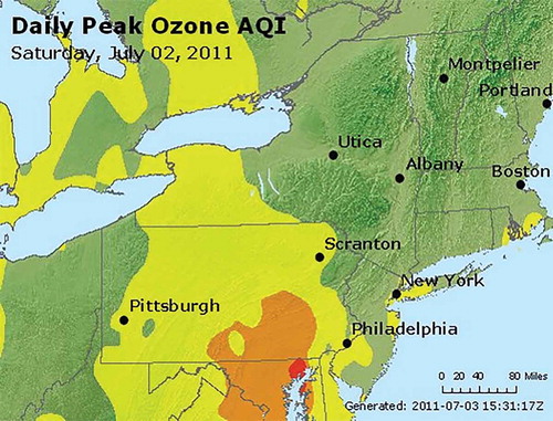
Heuristic or expert analysis has the possibility of adding value to the forecast guidance in cases where mesoscale effects are expected to affect the forecast. The last adjustment stage is the application of forecaster expertise. In the July 1 case summarized above, no air quality–relevant mesoscale effects were expected. As a result, the public forecast hewed to the guidance developed from the forecast rote. As shown in Table 1, the final expert forecast was 68 ppbv for the PHLFA, with 67 ppbv observed on July 1. The RIC area forecast underpredicted with Code Orange O₃ observed on July 1. On the two succeeding days, however, mesoscale effects became more influential. In 2011, the NAM NWP model operated with a12 km horizontal grid and its forecast for July 2, initialized on July 1 at 12:00 p.m. UTC, developed a sea breeze circulation during the day on July 2 with its leading edge reaching central New Jersey (Figure 13). The experience of air quality forecasters in the PHLFA is that air pollutants can pool west of sea or bay breeze boundaries with cleaner conditions to the east. The location of the sea breeze, and the strong O₃ or PM_2.5 gradients in its vicinity, is often poorly forecast by coarser-resolution meteorological models (Rao et al., 1999; Meir et al., 2013). In this case, however, forecaster experience suggested that sea breezes in July rarely penetrate beyond the center of New Jersey. The forecasters were faced with a NWP forecast that met expectations but an NAQP forecast that did not develop high O₃ mixing ratios in the expected location just west of the boundary. As a result, the expert forecast increased concentrations into the Code Orange range and warnings were issued. Observations on July 2 placed the sea breeze much further west than forecast, with radar imagery (not shown) showing the sea breeze from crossing the Delaware River and into Philadelphia County by early afternoon. As a result, the highest O₃ levels occurred just west and south of the PHLFA (Figure 14) and the expert forecast overpredicted peak O₃ (Table 3). However, unhealthy levels of O₃ were widespread across Maryland and central Pennsylvania on July 2, with the zone of Code Orange O₃ reaching to within 25–30 km of the nearest PHLFA monitors. In this case, the error was due to the misplacement of the sea breeze boundary.

Table 3. As in Table 1 but for the PHLFA only, July 2–3, 2011 (all measure in ppbv).

Parameter	July 2	July 3
Adjusted local persistence	67	68
Adjusted transport persistence	42	90
Sentinel monitor average	62	70
NAQFC	65	58
Ensemble of NAQP models	70	60
Range of NAQP models	[65, 76]	[58, 71]
Statistical model (Backcast)	66.3	54.5
Expert forecast	82	72
Observed domain maximum	68	76
Median of all monitors	63	59

Figure 13. Forecast 10 m wind speed (kts) and streamlines for 6:00 p.m. UTC, July 2, 2011. The NCEP WRF model was initialized at 12:00 p.m. UTC on July 1 (30-hr forecast). Figure courtesy of the Penn State Department of Meteorology (eWall, 2015).

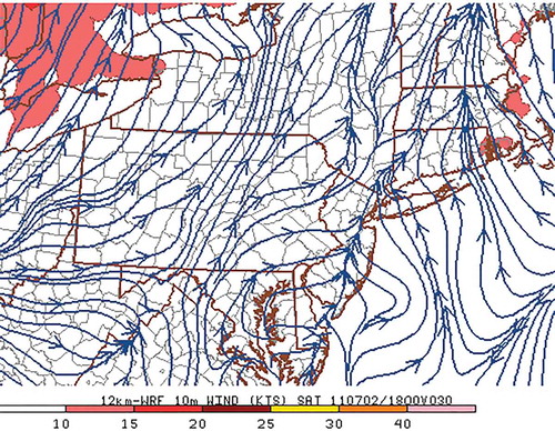
Figure 14. Daily peak O₃ Air Quality Index (AQI) for July 2, 2011. Image courtesy of EPA AirNow (EPA, 2015b).

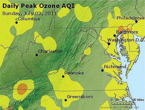
The following day, July 3, all the NWP models predicted that convection would occur during both the early morning and mid-afternoon hours, with the related NAQP models predicting much lower O₃. Forecaster experience has been that, contrary to model guidance and intuition, early morning convective activity has very little impact on late day O₃ peaks. As a result, forecasters discounted the very low O₃ model forecasts and focused on the timing and extent of late day convection. Because O₃ in the eastern U.S. has a broad maximum from 3:00 to 10:00 p.m. UTC, the timing of convection is critical. Early afternoon convection leads to much cleaner conditions, particularly with respect to O₃. Convection reduces O₃ through several mechanisms. First, cloud cover associated with anvils and cumulonimbus acts to decrease short-wave radiation and photochemical activity. Next, although O₃ is only slightly soluble in water (Henry’s law coefficient, H ~ O(10⁻²)), many other components of the O₃ production cycle are very soluble (e.g., HO_x, VOCs). Washout and rainout associated with convection effectively limit further O₃ production. Finally, outflow boundaries can influence O₃ even at large distances from the center of deep convection. In these instances, convective downdraft and updraft couplets act to exchange very clean mid-tropospheric air with polluted boundary layer air (Dickerson et al., 1987). The key issue for the air quality forecast on July 3 was the timing, location, and intensity of convection. In these cases, direct output from a number of NWP models can often be of more value for the air quality forecast than the NAQP models. In the operational setting, NWP models are available much sooner than the NAQP models and can be easily interrogated to determine stability parameters as well as dynamic forcing. In practice, operational air quality forecasters make use of profile visualization and analysis tools such as BUFKIT to assess local convective risk (Mahoney and Niziol, 2015). In the July 3 case, the NWP models predicted sufficient low-level moisture, convergence, and mid-level instability to support convection, although the dynamic forcing aloft was limited. Because the timing of precipitation varied from model to model, and from run to run, the expert forecast adjustment relied on the Short Range Ensemble Forecast (SREF) ensembles that developed convection early in the afternoon (Figure 15). Given the uncertainty in the timing of convection and the expected carry over of persistence O₃, the forecast (72 ppbv) was set higher than the ensemble NAQP model O₃ forecasts (60 ppbv). The NAQP model forecasts appeared to be influenced by early-day convection and persistent cloud cover. As it turned out, cloud cover was limited after 3:00 p.m. UTC. Convection developed as expected but was slightly (2–3 hr) delayed, and a gap in the convective activity was present over northern Delaware and southeastern Pennsylvania (Figure 16). High levels of persistence O₃ allowed scattered locations (five monitors) to record hourly concentrations ≥76 ppbv early in the afternoon, but strong convection prevented further increases. The highest O₃ levels were observed in a convection-free zone in northeastern Maryland and northern Delaware where an 8-hr average peak of 76 ppbv was reached (Figure 17). The expert forecast (72 ppbv) was 4 ppbv less than the domain maximum, although it was in the range of the four highest monitors [68, 76]. The impact of convection was clearly observed at the Bristol, Pennsylvania, and Rider University, New Jersey, monitors, near the Pennsylvania–New Jersey border north-northeast of PHL, where O₃ mixing ratios dropped 23 and 22 ppbv, respectively, in a single hour. In all, seven monitors logged 1-hr declines of >10 ppbv during the mid-late afternoon—a time when O₃ production is often maximized.

Figure 15. SREF 3-hr probability of measurable precipitation (in %) valid 6:00 p.m. UTC, July 3, 2011. SREF initialized 09:00 a.m. UTC, July 2, 2011. Figure courtesy of Penn State Department of Meteorology (eWall, 2015).

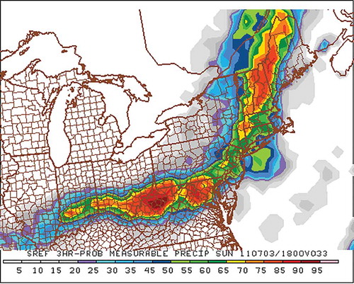
Figure 16. Radar composite image for 9:53 p.m. UTC, July 3, 2011. Figure courtesy of the University Center for Atmospheric Research (UCAR, 2015).

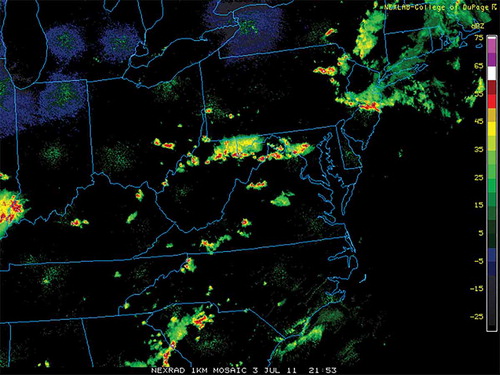
Figure 17. As in Figure 14 but for July 3, 2011.

Conclusion: The future forecast rote

Changes in the air quality forecast rote are expected to continue in the coming decade. Many of these changes will be driven by improvements in operational NWP and NAQP models. Forecasters will certainly applaud improvement in NAQP models, particularly for forecasts of PM_2.5. The most likely avenues for developments in the forecast rote will be related to increased model resolution, tighter coupling of offline models, operational implementation of online NAQP models, the incorporation of chemical data assimilation techniques, and the operational implementation of new postprocessing methods. A few comments from the operational forecaster perspective are given here.

Historically, the resolution of NAQP models has been determined by the resolution of its related meteorological model and the chemical emissions fields. Improving the resolution of the emissions fields is a difficult task, but chemical data assimilation, particularly the use of satellite-derived products, offers an avenue for improvement (Bocquet et al., 2015; Lu et al., 2015). Increases in NAQP model resolution, on the other hand, will be realized in the short term. At the current time, operational NWP models are routinely run at 4 km horizontal resolution with vertical resolution in excess of 50 layers. The expectation is that offline NAQP models will adopt this resolution and do so in the context of a more tightly coupled model system. At finer resolutions, a variety of air quality–relevant mesoscale effects are likely to be more accurately represented. For example, land-sea circulations (bay and sea breezes) are better resolved at horizontal resolutions of 4 km or less (Loughner et al., 2011, 2014). As noted in the example case of July 2 above, knowledge of the location and movement of land-sea circulation boundaries can inform air quality forecasts even in the absence of clear chemical model guidance.

An additional impact of finer-resolution NAQP models is the transition to “convection-allowing” systems. Current NAQP models rely on parameterization schemes in order to resolve convective activity. Higher-resolution models will allow convection to be resolved on the grid itself and promises, over time, better simulation of the timing, strength, and extent of convection. The interaction of convection with air quality is a source of great uncertainty, as seen above in the example case of July 3. Passing these improvements in convection simulation to air quality forecasts is likely to occur at a deliberate pace. First, the forecast latency period for air quality forecasts places a higher burden on convection forecasting. The primary impact of convection on air quality occurs during the afternoon hours of the following day, so that the convection forecast is effectively valid at time scales >24 hr. Skill in convection forecasts tends to decrease with time. Second, even though convection-allowing models dispense with a host of parameterization methods, the forcing of convection is still strongly affected by the simulation of planetary boundary layer (PBL) processes, which are themselves highly parameterized. For example, the transition from clear skies to shallow convection, which has a minimal impact on air quality, to deep convection that has a profound impact cannot be accurately resolved without properly simulating the PBL. Pollutant transport processes are also impacted by the accuracy of the PBL simulation. For example, transport by the nocturnal LLJs above the eastern U.S. coastal plain is a common phenomenon in poor air quality events. Although fine-resolution models should more accurately represent LLJs, the strength and vertical extent of the jet are subject to the accurate simulation of the nocturnal stable layer. The simulation of the nocturnal stable layer is still a challenging issue (Nunalee and Basu, 2014; Schepanski et al., 2014).

Implementation of operational online models is ongoing, particularly in Europe (see, for example, table 3 in Zhang et al., 2012a), and this trend will continue worldwide. The use of online models, which allow feedback between the meteorological and chemistry models, is likely to improve the skill of integrated PM_2.5 and O₃ forecast models as well as the simulation of radiative effects overall. An important limit on the operational use of online NAQP models has been computational resources. This constraint is likely to relax as computational power increases in the coming decade. The use of ensemble air quality models is also related to computational requirements, but its advent is likely to be significantly further in the future. Although NWP models currently use ensembles with a large number of members (~10¹–10²), the computation requirements of NAQP models are so much larger that only a few ensemble members are likely to be computable in the operational time frame in the near future—although multimodel ad hoc ensembles are currently in use operationally and could be expanded. In addition, it is not yet clear how to determine the optimal mix of ensemble members. In current NWP short-range model ensembles, the members are typically selected to characterize the uncertainty resulting from forcing due to initial condition errors and the impact of parameterization (e.g., convection and PBL) schemes. NAQP models must also address forcing due to boundary conditions and emissions fields that continue well past the time of model initialization (Vira and Sofiev, 2012; Bocquet et al., 2015).

The final area of future developments in the forecast rote is the operational implementation of sophisticated postprocessing techniques. In theory, a Model Output Statistics (MOS)-based approach holds the most promise. However, in the near future, a MOS approach will be difficult to apply in air quality applications. The development of a MOS training database requires a “frozen” forecast model. That is, the model on which the statistics are trained must be more or less identical throughout the historical period of interest. This may not be a strong constraint for the meteorological model, but the recent rate of changes in emissions assures that the model system as a whole will not be frozen for the appropriate length of time to develop MOS statistics. Techniques have been developed to use shorter time series—the Updateable MOS (UMOS) (Wilson and Vallee, 2003; Antonopoulos et al., 2012). In addition, using reanalysis data and reforecasting using the current model, or blend of models, is a possibility for further improvement (Hamill et al., 2015). In the short term, a variety of bias correction techniques have been used (Delle Monache et al., 2008; Kang et al., 2008; Neal et al., 2014). In 2015, a Kalman filter/analogue technique was tested for PM_2.5 model forecasts (Djalalova et al., 2015). This approach showed skill as applied in the PHLFA.

Conclusion

Over the past two decades, air quality forecasting techniques have evolved dramatically from a process dependent on diagnostics and empirical techniques to methods that emphasize guidance from numerical forecast models. The coming decade is likely to see further advances in forecast methods and accompanying changes to the operational forecast rote. In the short term, increases in forecast model resolution and more sophisticated postprocessing techniques will drive the most evident changes. There will be some lag in the impact of these changes as operational forecasters become “calibrated” to the behavior of the new models, but forecast skill, particularly in PM_2.5 forecasting, is likely to improve. In the longer term, the introduction of tightly coupled offline meteorology-chemistry models, or fully coupled online models, along with improvements in four-dimensional chemical data assimilation techniques, will result in future improvements in air quality forecasts. It is expected that the rapid changes in the forecast rote observed over the past decade will continue in the coming decades.

Additional information

Notes on contributors

William F. Ryan

William F. Ryan is a research scientist in the Department of Meteorology at the Pennsylvania State University.

References

- Antonopoulos, S., P. Bourgouin, J. Montpetit, and G. Croteau. 2012. Forecasting O3, PM2.5 and NO2 hourly spot concentrations using an updatable MOS methodology. In Air Pollution Modeling and Its Application XXI, ed. D.G Steyn and S.T. Rao, 309–314. Dordrecht, The Netherlands: Springer.
- Appel, K.W., C. Chemel, S.J. Roselle, X.V. Francis, R.-M. Hu, R.S. Sokhi, S.T. Rao, and S. Galmarini. 2012. Examination of the Community Multiscale Air Quality (CMAQ) model performance over the North American and European domains. Atmos. Environ. 53:142–155. doi:10.1016/j.atmosenv.2011.11.016
- Aron, R.H. 1980. Forecasting high level oxidant concentrations in the Los Angeles basin. J. Air Pollut. Control Assoc. 20:1227–1228.doi:10.1080/00022470.1980.10465174
- Black, T.L. 1994. The new NMC mesoscale Eta model: Description and forecast examples. Weather Forecast. 9:265–278. doi:10.1175/1520-0434(1994)009<0265:TNNMEM>2.0.CO;2
- Bocquet, M., H. Elbern, H. Eskes, M. Hirtl, R. Žabkar, G.R. Carmichael, J. Flemming, A. Inness, M. Pagowski, J.L. Pérez Camaño, and P.E. Saide. 2015. Data assimilation in atmospheric chemistry models: Current status and future prospects for coupled chemistry meteorology models. Atmos. Chem. Phys. Discuss. 14:32233–32323.doi:10.5194/acpd-14-32233-2014
- Burrows, W.R., M. Benjamin, S. Beauchamp, E.R. Lord, D. McCollor, and B. Thomson. 1995. CART decision-tree statistical analysis and prediction of summer season maximum surface ozone for the Vancouver, Montreal and Atlantic regions of Canada. J. Appl. Meteorol. 34:1848–1862. doi:10.1175/1520-0450(1995)034<1848:CDTSAA>2.0.CO;2
- Butler, T. J., F. M. Vermeylen, M. Rury, G.E. Likens, B. Lee, G. E. Bowker, and L. McCluney. 2011. Response of ozone and nitrate to stationary source NOx emission reductions in the eastern USA. Atmos. Environ. 45:1084–1094. doi:10.1016/j.atmosenv.2010.11.040
- Byun, D., and K. L. Schere. 2006. Review of the governing equations, computational algorithms, and other components of the Models-3 Community Multiscale Air Quality (CMAQ) modeling system. Appl. Mech. Rev. 59:51–77. doi:10.1115/1.2128636
- Cascio, W. E., A. Davis, and S. L. Stone. 2013. The Green Heart Initiative: Using air quality information to reduce adverse health effects in patients with heart and vascular disease. J. Cardiovasc. Nurs. 28:401–404. doi:10.1097/JCN.0b013e318295d1ae
- Chuang, M. T., Y. Zhang, and D. Kang. 2011. Application of WRF/Chem-MADRID for real-time air quality forecasting over the Southeastern United States. Atmos. Environ. 45:6241–6250. doi:10.1016/j.atmosenv.2011.06.071
- Cobourn, W. G. 2007. Accuracy and reliability of an automated air quality forecast system for ozone in seven Kentucky metropolitan areas. Atmos. Environ. 41:5863–5875. doi:10.1016/2007.03.024
- Cobourn, W. G., L. Dolcine, M. French, and M. C. Hubbard. 2000. A comparison of nonlinear regression and neural network models for ground-level ozone forecasting. J. Air Waste Manage. Assoc. 50:1999–2009. doi:10.1080/10473289.2000.10464228
- Cobourn, W.G., and M. C. Hubbard. 1999. An enhanced ozone forecasting model using air mass trajectory analysis. Atmos. Environ. 33:4663–4674. doi:10.1016/S1352-2310(99)00240-X
- Comrie, A.C. 1997. Comparing neural networks and regression models for ozone forecasting. J. Air Waste Manage. Assoc. 47:653–663. doi:10.1080/10473289.1997.10463925
- Cooper, O. R., R. S. Gao, D. Tarasick, T. Leblanc, and C. Sweeney. 2012. Long-term ozone trends at rural ozone monitoring sites across the United States, 1990–2010. J. Geophys. Res. 117(D22):D22307. doi:10.1029/2012JD018261
- Delle Monache, L., J. Wilczak, S. McKeen, G. Grell, M. Pagowski, S. Peckham, R. Stull, J. McHenry, and J. McQueen. 2008. A Kalman-filter bias correction method applied to deterministic, ensemble averaged and probabilistic forecasts of surface ozone. Tellus B 60:238–249. doi:10.1111/j.1600-0889.2007.00332.x
- Dickerson, R. R., G.J. Huffman, W.T. Luke, L.J. Nunnermacker, K.E. Pickering, et al. 1987. Thunderstorms: An important mechanism in the transport of air pollutants. Science 235:460–464. doi:10.1126/science.235.4787.460
- Djalalova, I., L. Delle Monache, and J. Wilczak. 2015. PM2.5 analog forecast and Kalman filter post-processing for the Community Multiscale Air Quality (CMAQ) model. Atmos. Environ. 108:76–87. doi:10.1016/j.atmosenv.2015.05.058
- Djalalova, I., J. Wilczak, S. McKeen, G. Grell, S. Peckham, M. Pagowski, L. Delle Monache, et al. 2010. Ensemble and bias-correction techniques for air quality model forecasts of surface O3 and PM2.5 during the TEXAQS-II experiment of 2006. Atmos. Environ. 44:455–467. doi:10.1016/j.atmosenv.2009.11.007
- Doraiswamy, P., C. Hogrefe, W. Hao, K. Civerolo, J.-Y. Ku, and G. Sistla. 2010. A retrospective comparison of model-based forecasted PM2.5 concentrations with measurements. J. Air Waste Manage. Assoc. 60:1293–1308. doi:10.3155/1047-3289.60.11.1293
- Doswell, C.A., III. 2004. Weather forecasting by humans—Heuristics and decision making. Weather Forecast. 19:1115–1126. doi:10.1175/WAF-821.1
- Draxler, R. R., and G. D. Hess. 1998. An overview of the HYSPLIT_4 modeling system of trajectories, dispersion, and deposition. Aust. Meteor. Mag. 47:295–308.
- Draxler, R. R., and G. D. Rolph. 2015. HYSPLIT (HYbrid Single-Particle Lagrangian Integrated Trajectory). Model access via NOAA ARL READY Web site. NOAA Air Resources Laboratory, Silver Spring, MD. http://ready.arl.noaa.gov/HYSPLIT.php (accessed October 27, 2015).
- Eder, B., D. Kang, R. Mathur, J. Pleim, S. Yu, T. Otte, et al. 2009. A performance evaluation of the National Air Quality Forecast Capability for the summer of 2007. Atmos. Environ. 43:2312–2320. doi:10.1016/j.atmosenv.2009.01.033
- Eder, B., D. Kang, R. Mathur, S. Yu, and K. Schere. 2006. An operational evaluation of the Eta-CMAQ air quality forecast model. Atmos. Environ. 40:4894–4905. doi:10.1016/j.atmosenv.2005.12.062
- Elbern, H., and H. Schmidt. 2001. Ozone episode analysis by four dimensional variational chemistry data assimilation. J. Geophys. Res. 106:3569–3590. doi:10.1029/2000JD900448
- e-WALL: The Electronic Map Wall Product, copyright 2004–2016. 2015. eWall: The Electronic Wall Map. Department of Meteorology, The Pennsylvania State University, University Park, PA. http://mp1.met.psu.edu/~fxg1/ewall.html (accessed October 27, 2015).
- Garner, G. G., and A. M. Thompson. 2012. The value of air quality forecasting in the mid-Atlantic region. Weather Climate Soc. 4:69–79. doi:10.1175/WCAS-D-10-05010.1
- Gaza, R. S. 1998. Mesoscale meteorology and high ozone in the northeast United States. J. Appl. Meteorol. 37:961–977. doi:10.1175/1520-0450(1998)037<0961:MMAHOI>2.0.CO;2
- Gilliland, A. B., et al. 2008. Dynamic evaluation of regional air quality models: Assessing changes in O3 stemming from changes in emissions and meteorology. Atmos. Environ. 42:5110–5123. doi:10.1016/j.atmosenv.2008.02.018
- Godowitch, J. M., A. B. Gilliland, R. R. Draxler, and S. T. Rao. 2008a. Modeling assessment of point source NOx emission reductions on ozone air quality in the eastern United States. Atmos. Environ. 42:87–100. doi:10.1016/j.atmosenv.2007.09.032
- Godowitch, J. M., C. Hogrefe, and S. T. Rao. 2008b. Diagnostic analyses of a regional air quality model: Changes in modeled processes affecting ozone and chemical-transport indicators from NOx point source emission reductions. J. Geophys. Res. 113(D19):D19303. doi:10.1029/2007JD009537
- Godowitch, J.M., Pouliot, G. A., and S. T. Rao. 2010. Assessing multi-year changes in modeled and observed urban NOx concentrations from a dynamic model evaluation perspective. Atmos. Environ. 44:2894–2901. doi:10.1016/j.atmosenv.2010.04.040
- Grell, G., and A. Baklanov. 2011. Integrated modeling for forecasting weather and air quality: A call for fully coupled approaches. Atmos. Environ. 45:6845–6851. doi:10.1016/j.atmosenv.2011.01.017
- Grell, G. A., S. E. Peckham, R. Schmitz, S. A. McKeen, G. Frost, W. C. Skamarock, and B. Eder. 2005. Fully coupled “online” chemistry within the WRF model. Atmos. Environ. 39:6957–6975. doi:10.1016/j.atmosenv.2005.04.027
- Hamill, T. M., K. Gilbert, and M. Peroutka. 2015. Statistical post-processing in NOAA: Key changes necessary to make the national blend of models and reforecasting successful. http://www.esrl.noaa.gov/psd/people/tom.hamill/WhitePaperImplementationofReforecastsandNationalBlend.pdf (accessed November 2, 2015).
- Hanna, S. R., Z. Lu, H. C. Frey, N. Wheeler, J. Vukovich, S. Arunachalam, M. Fernau, and D. A. Hansen. 2001. Uncertainties in predicted ozone concentrations due to input uncertainties for the UAM-V photochemical grid model applied to the July 1995 OTAG domain. Atmos. Environ. 35:891–903. doi:10.1016/S1352-2310(00)00367-8
- He, H., J. W. Stehr, J. C. Hains, D. J. Krask, B. G. Doddridge, K. Y. Vinnikov, T. P. Canty, et al. 2013. Trends in emissions and concentrations of air pollutants in the lower troposphere in the Baltimore/Washington airshed from 1997 to 2011. Atmos. Chem. Phys. 13:7859–7874. doi:10.5194/acp-13-7859-2013
- Hu, X.-M., P. M. Klein, M. Xue, F. Zhang, D. C. Doughty, R. Forkel, E. Joseph, and J. D. Fuentes. 2013. Impact of the vertical mixing induced by low-level jets on boundary layer ozone concentration. Atmos. Environ. 70:123–130. doi:10.1016/j.atmosenv.2012.12.046
- Im, U., R. Bianconi, E. Solazzo, I. Kioutsioukis, A. Badia, A. Balzarini, R. Baró, et al. 2015. Evaluation of operational online-coupled regional air quality models over Europe and North America in the context of AQMEII phase 2. Part I: Ozone. Atmos. Environ. 115:404–420. doi:10.1016/j.atmosenv.2014.09.042
- Janjic, Z.I. 2003. A nonhydrostatic model based on a new approach. Meteorol. Atmos. Phys. 82:271–285. doi:10.1007/s00703-001-0587-6
- Kang, D., R. Mathur, R., S. T. Rao, and S. Yu. 2008. Bias adjustment techniques for improving ozone air quality forecasts. J. Geophys. Res. 113(D23): D23308. doi: 10.1029/2008JD010151.
- Klein, W. H. 1971. Computer prediction of precipitation probability in the United States. J. Appl. Meteorol. 10:903–915. doi:10.1175/1520-0450(1971)010<0903:CPOPPI>2.0.CO;2
- Kukkonen, J., T. Olsson, D. M. Schultz, A. Baklanov, Thomas Klein, A. I. Miranda, A. Monteiro, et al. 2012. A review of operational, regional-scale, chemical weather forecasting models in Europe. Atmos. Chem. Phys. 12:1–87. doi:10.5194/acp-12-1-2012
- Lee, P., et al. 2012. Incremental development of air quality forecasting system with offline/online capability: Coupling CMAQ to NCEP national mesoscale model. In Air Pollution Modeling and Its Application XXI ed. D.G Steyn and S.T. Rao, 187–192. Dordrecht, The Netherlands: Springer.
- Loughner, C. P., D. J. Allen, K. E. Pickering, D.-L. Zhang, Y.-X. Shou, and R. R. Dickerson. 2011. Impact of fair-weather cumulus clouds and the Chesapeake Bay breeze on pollutant transport and transformation. Atmos. Environ. 45:4060–4072. doi:10.1016/j.atmosenv.2011.04.003.
- Loughner, C. P., et al. 2014. Impact of bay-breeze circulations on surface air quality and boundary layer export. J. Appl. Meteorol. 53:1697–1713. doi:10.1175/JAMC-D-13-0323.1
- Lu, Z., D. G. Streets, B. de Foy, L. N. Lamsal, B. N. Duncan, and J. Xing. 2015. Emissions of nitrogen oxides from US urban areas: Estimation from Ozone Monitoring Instrument retrievals for 2005–2014. Atmos. Chem. Phys. 15:14961–15003. doi:10.5194/acpd-15-14961-2015
- Mahoney, E. A., and T. A. Niziol. 1997. BUFKIT: A software application toolkit for predicting lake-effect snow. Preprints, 13th Intl. Conf. on Interactive Information and Processing Systems for Meteorology, Oceanography, and Hydrology. Long Beach, CA, Amer. Meteor. Soc., 388–391.
- McCollister, G., and K. Wilson. 1975. Linear stochastic models for forecasting daily maxima and hourly concentrations of air pollutants. Atmos. Environ. 9:417–423. doi:10.1016/0004-6981(75)90127-4
- McHenry, J. N., W. F. Ryan, N.L. Seaman, C.J. Coats Jr., J. Pudykiewicz, S. Arunachalam, J.M. Vukovich, et al. 2004. A real-time Eulerian photochemical model forecast system: Overview and initial ozone forecast performance in the northeast US corridor. Bull. Am. Meteorol. Soc. 85:525–548. doi:10.1175/BAMS-85-4-525
- McHenry, J. N., N. Seaman, C. Coats, A. Lario-Gibbs, J. Vukovich, N. Wheeler, and E. Hayes. 1999. Real-time nested mesoscale forecasts of lower tropospheric ozone using a highly optimized coupled model numerical prediction system. In Symposium on Interdisciplinary Issues in Atmospheric Chemistry, 125–128.
- McKeen, S., G. Grell, S. Peckham, J. Wilczak, I. Djalalova, E.-Y. Hsie, et al. 2009. An evaluation of real-time air quality forecasts and their urban emissions over eastern Texas during the summer of 2006 Second Texas Air Quality Study field study. J. Geophys. Res. 114(D7): D00F11. doi: 10.1029/2008JD011697.
- McKeen, S., J. Wilczak, G. Grell, I. Djalalova, S. Peckham, E.-Y. Hsie, W. Gong, et al. 2005. Assessment of an ensemble of seven real-time ozone forecasts over eastern North America during the summer of 2004. J.Geophys. Res. 110(D21):D21307. doi: 10.1029/2005JD005858.
- Meir, T., P. M. Orton, J. Pullen, T. Holt, W. T. Thompson, and M. F. Arend. 2013. Forecasting the New York City urban heat island and sea breeze during extreme heat events. Weather Forecast. 28:1460–1477. doi:10.1175/WAF-D-13-00012.1
- National Center for Environmental Prediction. 2015. National Center for Environmental Prediction (NCEP), Environmental Modeling Center, Washington, DC. NCEP operational air quality forecast change log. http://www.emc.ncep.noaa.gov/mmb/aq/AQChangelog.html ( accessed October 27, 2015).
- Neal, L. S., P. Agnew, S. Moseley, C. Ordóñez, N. H. Savage, and M. Tilbee. 2014. Application of a statistical post-processing technique to a gridded, operational, air quality forecast. Atmos. Environ. 98:385–393. doi:10.1016/j.atmosenv.2014.09.004
- Niemeyer, L. E. 1960. Forecasting air pollution potential. Mon. Weather Rev. 88:88–96. doi:10.1175/1520-0493(1960)088<0088:FAPP>2.0.CO;2
- Nunalee, C.G., and S. Basu. 2014. Mesoscale modeling of coastal low-level jets: Implications for offshore wind resource estimation. Wind Energy 17:1199–1216. doi:10.1002/we.v17.8
- Otte, T. L., and J. E. Pleim. 2010. The Meteorology-Chemistry Interface Processor (MCIP) for the CMAQ modeling system: Updates through MCIPv3. 4.1. Geosci. Model Dev. 3:243–256. doi:10.5194/gmd-3-243-2010
- Otte, T. L., G. Pouliot, J. E. Pleim, J. O. Young, K. L. Schere, D. C. Wong, P. S. Lee, et al. 2005. Linking the Eta model with the Community Multiscale Air Quality (CMAQ) modeling system to build a national air quality forecasting system. Weather Forecast. 20:367–384. doi:10.1175/WAF855.1
- Pagnotti, V. 1987. A meso-meteorological feature associated with high ozone concentrations in the northeastern United States. J. Air Pollut. Control Assoc. 37:720–722. doi:10.1080/08940630.1987.10466258
- Pan, L., D. Q. Tong, P. Lee, H. Kim, and T. Chai. 2014. Assessment of NOx and O3 forecasting performances in the U.S. National Air Quality Forecasting Capability before and after the 2012 major emissions updates. Atmos. Environ. 95:610–619. doi: 10.1016/j.atmosenv.2014.06.020
- Pielke, R. A., and M. Uliasz. 1998. Use of meteorological models as input to regional and mesoscale air quality models—Limitations and strengths. Atmos. Environ. 32:1455–1466. doi:10.1016/S1352-2310(97)00140-4
- Rao, P. A., H. E. Fuelberg, and K. K. Droegemeier. 1999. High-resolution modeling of the Cape Canaveral area land-water circulations and associated features. Mon. Weather Rev. 127:1808–1821. doi:10.1175/1520-0493(1999)127<1808:HRMOTC>2.0.CO;2
- Robeson, S. M., and D. G. Steyn. 1989. A conditional probability density function for forecasting ozone air quality data. Atmos. Environ. 23:689–692. doi:10.1016/0004-6981(89)90016-4
- Rogers, E., G. DiMego, T. Black, M. Ek, B. Ferrier, G. Gayno, Z. Janjic, et al. 2009. The NCEP North American mesoscale modeling system: Recent changes and future plans. In Preprints, 23rd Conference on Weather Analysis and Forecasting/19th Conference on Numerical Weather Prediction. Omaha, NE, Amer. Meteor. Soc., 2A.4., 1–5 June, 2009. http://ams.confex.com/ams/pdfpapers/154114.pdf.
- Ruiz-Suárez, J. C., O. A.Mayora-Ibarra, J. Torres-Jiménez, and L. G. Ruiz-Suárez. 1995. Short-term ozone forecasting by artificial neural networks, Adv. Eng. Softw. 23:143–149. doi:10.1016/0965-9978(95)00076-3
- Russell, A., and R. Dennis. 2000. NARSTO critical review of photochemical models and modeling. Atmos. Environ. 34:2283–2324. doi:10.1016/S1352-2310(99)00468-9
- Ryan, W. F. 1995. Forecasting ozone episodes in the Baltimore metropolitan area. Atmos. Environ. 29:2387–2398. doi:10.1016/1352-2310(94)00302-2
- Ryan, W. F. 2011. July 2011 episode summary. Department of Meteorology, Pennsylvania State University. http://www.meteo.psu.edu/~wfr1/July-2011-episode-summary.pdf (accessed October 27, 2015).
- Ryan, W. F., B. Doddridge, R. R. Dickerson, R. M. Morales, K. A. Hallock, P. T. Roberts, K. L. Civerolo, et al. 1998. Pollutant transport during a regional O3 episode in the Mid-Atlantic States. J. Air Waste Manage. Assoc. 48:786–797. doi:10.1080/10473289.1998.10463737
- Ryan, W.F., C. A. Piety, and E. D. Luebehusen. 2000. Air quality forecasts in the mid-Atlantic region: Current practice and benchmark skill. Weather Forecast. 15:46–60. doi:10.1175/1520-0434(2000)015<0046:AQFITM>2.0.CO;2
- Schaefer, J.T. 1986. Severe thunderstorm forecasting: A historical perspective. Weather Forecast. 1:164–189. doi:10.1175/1520-0434(1986)001<0164:STFAHP>2.0.CO;2
- Schepanski, K., et al. 2014. The sensitivity of nocturnal low-level jets and near-surface winds over the Sahel to model resolution, initial conditions and boundary-layer set-up. Q. J. R. Meteorol. Soc. 141:1442–1456. doi: 10.1002/qj.2453.
- Seaman, N. L. 2000. Meteorological modeling for air-quality assessments. Atmos. Environ. 34:2231–2259. doi:10.1016/S1352-2310(99)00466-5
- Seaman, N. L., and S. A. Michelson. 2000. Mesoscale meteorological structure of a high-ozone episode during the 1995 NARSTO-Northeast study. J. Appl. Meteorol. 39:384–398. doi:10.1175/1520-0450(2000)039<0384:MMSOAH>2.0.CO;2
- Stauffer, R. M., and A. M. Thompson. 2013. Bay breeze climatology at two sites along the Chesapeake Bay from 1986–2010: Implications for surface ozone. J. Atmos. Chem. 70:1–18. doi:10.1007/s10874-013-9260-y
- Stauffer, R. M., A. M. Thompson, D. K. Martins, R. D. Clark, D. L. Goldberg, C. P. Loughner, R. Delgado, R. R. Dickerson, J. W. Stehr, and M. A. Tzortziou. 2012. Bay breeze influence on surface ozone at Edgewood, MD during July 2011. J. Atmos. Chem. 69:1–19. doi:10.1007/s10874-012-9241-6
- Tang, Y., P. Lee, M. Tsidulko, H. Huang, J. T. McQueen, G. J. DiMego, L. K. Emmons, R. B. Pierce, A. M. Thompson, H. Lin, et al. 2008. The impact of chemical lateral boundary conditions on CMAQ predictions of tropospheric ozone over the continental United States. Environ. Fluid Mech. 9:43–58. doi: 10.1007/s10652-008-9092-5
- Taylor, E. 2014. The Canadian Air Quality Health Index. In Air Quality Management, ed. E. Taylor and A. McMillan, 351–363. Dordrecht, The Netherlands: Springer.
- Triangle Air Awareness. 2015. Triangle Air Awareness Web site. http://www.triangleairawareness.org (accessed October 28, 2915).
- University Center for Atmospheric Research. 2015. Image Archive. http://www2.mmm.ucar.edu/imagearchive (accessed October 27, 2015).
- U.S. Environment Protection Agency. 2003. Guidelines for Developing an Air Quality (Ozone and PM2.5) Forecasting Program. EPA-456/R-03-002. http://www3.epa.gov/airnow/aq_forecasting_guidance-1016.pdf (accessed December 19, 2015).
- U.S. Environment Protection Agency. 2010. Primary National Ambient Air Quality Standard for nitrogen dioxide. Fed. Regist. 75:6473–6537. http://www3.epa.gov/ttn/naaqs/standards/nox/fr/20100209.pdf (accessed December 19, 2015).
- U.S. Environment Protection Agency. 2015a. National Ambient Air Quality Standard for ozone. Fed. Regist. 80: 65292–65468.https://www.gpo.gov/fdsys/pkg/FR-2015-10-26/pdf/2015-26594.pdf (accessed December 19, 2015).
- U.S. Environment Protection Agency. 2015b. AirNow Program, Research Triangle Park, NC. http://www.airnow.gov (accessed October 26, 2015).
- Vautard, R., M. D. Moran, E. Solazzo, R. C. Gilliam, V. Matthias, R. Bianconi, C. Chemel, et al. 2012. Evaluation of the meteorological forcing used for the Air Quality Model Evaluation International Initiative (AQMEII) air quality simulations. Atmos. Environ. 53:15–37. doi:10.1016/j.atmosenv.2011.10.065
- Vira, J., and M. Sofiev. 2012. Comparing air quality forecast and a reanalysis: Improvements due to chemical data assimilation and better NWP forcing. In Air Pollution Modeling and its Application XXI, ed. D.G Steyn and S.T. Rao, 403–406. Dordrecht, The Netherlands: Springer.
- Weisman, R. A. 1990. An observational study of warm season southern Appalachian lee troughs. Part I: Boundary layer circulation. Mon. Weather Rev. 118:950–963. doi:10.1175/1520-0493(1990)118<0950:AOSOWS>2.0.CO;2
- Wen, X.-J., L. Balluz, and A. Mokdad. 2009. Association between media alerts of air quality index and change of outdoor activity among adult asthma in six states, BRFSS, 2005. J. Community Health 34:40–46. doi:10.1007/s10900-008-9126-4
- Wilczak, J., S. McKeen, I. Djalalova, G. Grell, S. Peckham, W. Gong, V. Bouchet, et al. 2006. Bias-corrected ensemble and probabilistic forecasts of surface ozone over eastern North America during the summer of 2004. J.Geophys. Res. 111(D23):D23528. doi:10.1029/2006JD007598
- Wilson, L. J., and M. Vallée. 2003. The Canadian updateable model output statistics (UMOS) system: Validation against perfect prog. Weather Forecast. 18:288–302. doi:10.1175/1520-0434(2003)018<0288:TCUMOS>2.0.CO;2
- Wolff, G.T., and P.J. Lioy. 1978. An empirical model for forecasting maximum daily ozone levels in the northeastern United States. J. Air Pollut. Control Assoc. 28:1034–1038. doi:10.1175/1520-0434(2003)018<0288:TCUMOS>2.0.CO;2
- Yu, S., R. Mathur, K.Schere, D. Kang, J. Pleim, and T. L. Otte. 2007. A detailed evaluation of the Eta-CMAQ forecast model performance for O3, its related precursors, and meteorological parameters during the 2004 ICARTT study. J. Geophys. Res. 112(D12): D12514. doi: 10.1029/2006JD007715.
- Yu, S., R. Mathur, K.Schere, D. Kang, J. Pleim, Young, J., et al. 2008. Evaluation of realtime PM2.5 forecasts and process analysis for PM2.5 formation over the eastern United States using the Eta-CMAQ forecast model during the 2004 ICARTT study. J. Geophys. Res. 113(D6): D06204. doi: 10.1029/2007JD009226.
- Zhang, D.-L., S. Zhang, and S. J. Weaver. 2006. Low-level jets over the Mid-Atlantic states: Warm-season climatology and a case study. J. Appl. Meteorol. 45:194–209. doi:10.1175/JAM2313.1
- Zhang, Y. 2008. Online-coupled meteorology and chemistry models: History, current status, and outlook. Atmos. Chem. Phys. 8:2895–2932. doi:10.5194/acp-8-2895-2008
- Zhang, Y., M. Bocquet, V. Mallet, C. Seigneur, and A. Baklanov. 2012a. Real-time air quality forecasting, Part I: History, techniques, and current status. Atmos. Environ. 60:632–655. doi:10.1016/j.atmosenv.2012.06.031
- Zhang, Y., M. Bocquet, V. Mallet, C. Seigneur, and A. Baklanov. 2012b. Real-time air quality forecasting, Part II: State of the science, current research needs, and future prospects. Atmos. Environ. 60:656–676. doi:10.1016/j.atmosenv.2012.02.041