Forecasting air quality time series using deep learning

ABSTRACT

This paper presents one of the first applications of deep learning (DL) techniques to predict air pollution time series. Air quality management relies extensively on time series data captured at air monitoring stations as the basis of identifying population exposure to airborne pollutants and determining compliance with local ambient air standards. In this paper, 8 hr averaged surface ozone (O₃) concentrations were predicted using deep learning consisting of a recurrent neural network (RNN) with long short-term memory (LSTM). Hourly air quality and meteorological data were used to train and forecast values up to 72 hours with low error rates. The LSTM was able to forecast the duration of continuous O₃ exceedances as well. Prior to training the network, the dataset was reviewed for missing data and outliers. Missing data were imputed using a novel technique that averaged gaps less than eight time steps with incremental steps based on first-order differences of neighboring time periods. Data were then used to train decision trees to evaluate input feature importance over different time prediction horizons. The number of features used to train the LSTM model was reduced from 25 features to 5 features, resulting in improved accuracy as measured by Mean Absolute Error (MAE). Parameter sensitivity analysis identified look-back nodes associated with the RNN proved to be a significant source of error if not aligned with the prediction horizon. Overall, MAE's less than 2 were calculated for predictions out to 72 hours.

Implications: Novel deep learning techniques were used to train an 8-hour averaged ozone forecast model. Missing data and outliers within the captured data set were replaced using a new imputation method that generated calculated values closer to the expected value based on the time and season. Decision trees were used to identify input variables with the greatest importance. The methods presented in this paper allow air managers to forecast long range air pollution concentration while only monitoring key parameters and without transforming the data set in its entirety, thus allowing real time inputs and continuous prediction.

Introduction

Tropospheric ozone (O₃) is a secondary pollutant formed by complex photochemical processes that impacts human health, plants, and structural materials. More than 21,000 premature deaths in Europe are attributed annually to O₃ exposure (Amann et al. 2008), with more than 1.1 million deaths worldwide—more than 20% of all deaths attributed to respiratory diseases (Malley et al. 2017). In cases where O₃ levels will exceed standards for long periods of time, air managers may issue air quality warnings and even limit industrial and vehicular activities (Kuhlbusch et al. 2014; Welch, Gu, and Kramer 2005). Improving forecast accuracy provides planning and decision options that can impact receptor health and local economies.

In this paper, we train a deep learning model, consisting of a recurrent neural network (RNN) with long short-term memory (LSTM), to accurately predict local 8-hr averaged (ave) O₃ concentrations based on hourly air monitoring station measurements as a tool to forecast air pollution. RNNs are particularly well suited for air concentration prediction because they incorporate sequential history into the training and processing of input data. Air quality measurements are time-series data sets in which the order of data is important. Tropospheric O₃ was chosen as a parameter to forecast because of its complex formation processes and sources.

Background

Ozone as an ambient air pollutant

The majority of tropospheric O₃ is generated through anthropogenic sources (Cooper et al. 2006; Lelieveld and Dentener 2000) attributed to the photo-disassociation of NO₂, as shown next in the simplified reaction (Finlayson-Pitts and Pitts 1993):

(1)

where M is a stabilization molecule used during the intermediate formation between O and O₂. In addition to nitrogen oxides (NOx’s), volatile organic compounds (VOCs), chlorine, solar radiation (SR), relative humidity (RH) and ambient temperature also impact tropospheric O₃ formation (Song et al. 2011). Local concentrations of O₃ are further influenced by weather patterns and terrain that disperse the pollutants, precursors, and by-products (Beck, Krzyzanowski, and Koffi 1998). At night, O₃ reacts with NO₂ to form NO3 (nitrate radical) (Finlayson-Pitts and Pitts 1993):

(2)

The NO₃ radicals react with NO₂ to form dinitrogen pentoxide (N₂O₅), which in turn forms nitric acid (HNO₃) through hydrolysis with water or aqueous particles (Song et al. 2011; Thornton et al. 2010). The acid is finally neutralized by ammonia (NH₃) to complete the reaction chain (Brown and Stutz 2012).

Additional contributions to tropospheric O₃ concentrations come from the stratosphere–troposphere exchange (STE) of stratospheric ozone (Tarasick and Slater 2008). The percentage of O₃ provided by STE at surface levels ranges from 13% (Cooper et al. 2006) to more than 42% (Lelieveld and Dentener 2000), depending on area and conditions. With so many chemical and transport phenomena taking place throughout the day and night, modeling O₃ becomes a very complex task even before local terrain, sources, and weather patterns are incorporated (Bei et al. 2014). Nonetheless, predicting ambient O₃ concentrations, and in particular, concentrations that may exceed air quality standards, is important for air managers and at-risk populations.

Forecasting ozone with machine learning

Due to the formation process of O₃, the actual concentration a local population is exposed to may have been generated from precursors emitted hundreds or even thousands of kilometers away (Glavas and Sazakli 2011). Populations living in coastal regions may be exposed to pollutants generated locally but transformed and mixed with other precursors in circulating land–sea breezes (Freeman et al. 2017a). Tropospheric O₃ is therefore a more complex pollutant to estimate than primary pollutants such as sulfur dioxide (SO₂) or carbon monoxide (CO).

Many studies have used supervised machine learning techniques, such as artificial neural networks (ANNs) to predict O₃ time-series concentrations (Biancofiore et al. 2017; Ettouney et al. 2009; Kurt et al. 2008; Wirtz et al. 2005). ANNs have been shown to provide better predictive results than linear models such as multiple linear regression (MLR) and time-series models such as autoregressive integrated moving averages (ARIMA) (Liu 2007; Prybutok, Yi, and Mitchell 2000; Vlachogianni et al. 2011; Zickus, Greig, and Niranjan 2002). Support vector machines (SVMs) have also been applied to O₃ prediction scenarios with results that often outperform ANNs (Luna et al. 2014; Papaleonidas and Iliadis 2013; Singh, Gupta, and Rai 2013).

The benefits of using ANNs include not requiring a priori assumptions of the data used for training and not requiring weighting of initial inputs (Gardner and Dorling 1998). In practice, dimensionality reduction is often used to remove inputs to the model that are not independent and identically distributed (IID) or offer little influence on the overall training. Principal component analysis (PCA) is often used to reduce the overall inputs to the model by removing transformed components, but provides little variability to the actual number of features required to train (Singh, Gupta, and Rai 2013; Wang et al. 2015).

Most of the studies that use ANNs apply a single hidden-layer feed forward neural network (FFNN) architecture trained with meteorological and concentration data and have limited success in forecasting air quality. The canonical FFNN model consists of an input layer, a hidden layer, and an output layer. Each layer is constructed from interlinked nodes that generate a value (usually between −1 and 1 or between 0 and 1). The individual node model is shown in Figure 1.

Figure 1. Individual node model.

The node sums the weighted inputs of the previous layer, sometimes with a bias, and transforms the combined sum with a nonlinear activation function, σ. The node activation equation is given by

(3)

where w is an array of weights for the connections between the previous layer and the current layer, x is a vector of input values from the previous layer, and b is a bias value. Common activation functions include the sigmoid, tanh, and relu functions. A general property for activation functions is that they normalize the output and have a continuous first-order derivative that can be used during the back-propagation training process (Goodfellow, Bengio, and Courville 2016). The common activation functions mentioned earlier are shown in Table 1 along with their first-order derivative and output range.

Table 1. Common activation functions.

Name	Equation	First derivative	Output range
sigmoid
tanh			−1, 1
relu

More recent studies, however, looked at the limitations of FFNNs, namely, the difficulty in choosing a suitable architecture and the tendency to overfit the training data, leading to poor generalization, particularly in situations where limited labeled data are available (Lu and Wang 2005; Papaleonidas and Iliadis 2013). The predicted outputs in previous air quality forecast studies (Arhami, Kamali, and Rajabi 2013) were based on continuous concentration values measured in parts per billion (ppb) or micrograms per cubic meter (μg/m³) from single stations. Achar et al. (2011) investigated the intervals between O₃ exceedances and maxima of daily concentration levels instead of estimating real-time values. Their study of interoccurrence between peaks was used to determine overall improvements in air quality trends over time as compared to predicting future air quality concentrations (Achcar et al., 2011).

For our validation case study area in Kuwait, several studies were completed that focused on ambient air quality and modeling using ANNs. Abdul-Wahab (2001) used 5-min measurements of precursors (CH₄, nonmethane hydrocarbons (NMHCs), CO, CO₂, dust, NO, NO₂, and NOx) and meteorological inputs (wind speed [WS], wind direction [WD], temperature [TEMP], RH, and solar radiation) from a mobile site in the Khaldiya residential area to estimate ozone and smog produced (SP) using a single hidden layer FFNN (Abdul-Wahab 2001). Al-Alawi and Abdul-Wahab later enhanced their model by applying PCA to reduce the dimensionality of the input data (Al-Alawi, Abdul-Wahab, and Bakheit 2008). Ettouney et al. (2009) used the same inputs as Abdul-Wahab (replacing dust with methanated hydrocarbons) and two FFNNs to predict monthly O₃ concentrations from the Jahra and Um Al Hayman stations. They suggested that O₃ in Kuwait often comes from outside the local area via long-range transport (Ettouney et al. 2009).

Deep learning and time series

Studies in atmospheric sciences and O₃ concentration predictions using deep learning (DL) have not been as common as single hidden layer ANNs. DL refers to the families of ANNs that have more than one hidden layer or use advanced architectures such as recurrent neural networks (RNNs) and convolutional neural networks (CNNs) (Goodfellow, Bengio, and Courville 2016). Partially recurrent network models, such as the Elman network (EN), were used with air station inputs to predict ground-level concentrations of O₃ (Biancofiore et al. 2015) and PM_2.5 (Biancofiore et al. 2017). The feedback provides memory to the system when a single input set is fed into the system. Different ANN architectures are shown in Figure 2. The simple node in Figure 1 is redrawn as a circle for comparison. The arrows between layers represent synaptic weights that interconnect each node. Figure 2 shows that each layer can have different numbers of nodes; however, the numbers of nodes in deep neural networks (DNNs) hidden layers are usually kept the same for each layer.

Figure 2. Different ANN model architectures: (a) simple feed-forward neural network, (b) a recurrent (Elman) neural network, and (c) a deep feed-forward neural network with multiple hidden layers.

Implementations of procedures such as LSTM for RNNs allow network training to take place without having long-term parameters “explode” or “vanish” as a result of multiple learning updates (Pascanu, Mikolov, and Bengio 2013). LSTM was first introduced by Hochreiter and Schmidhuber in 1997 to overcome these training issues (Hochreiter and Schmidhuber 1997). Gomez was one of the first researchers to use a single-layer RNN to forecast maximum ozone concentrations in Austria (Gomez et al. 2003). His model utilized LSTM to outperform other architectures such as ENs. Noting the gap of years from Gomez et al. in 2003 and the work by Biancofirore et al. as recently as 2017 using ENs shows that the complexity of preparing and training RNNs that use LSTM has kept researchers from using DL methods. DL has recently become popular for many applications due to improvements in training procedures and software libraries such as Theano (Theano Development Team 2016) and Keras (Chollet et al., 2015) and Tensorflow (Abadi et al. 2015). These libraries have made implementing DL models easier, and therefore more accessible for researchers outside of the machine learning fields. A discussion of the theory of RNNs is presented in the next section.

Theoretical approach

Time series data

Air quality data are continuous, multivariate time series where each reading constitutes a set measurement of time and the current reading is in some way related to the previous reading, and therefore dependent (Gheyas and Smith 2011). Measured pollutants may be related through photochemical or precursor dependencies, while meteorological conditions are limited by physical properties. Time series are often impacted by collinearity and nonstationarity that also violate independence assumptions and can make forecast modeling difficult (Gheyas and Smith 2011). Autocorrelation of individual pollutants shows different degrees of dependence to past values. Correlation coefficients were calculated using the equation

(4)

where X is the input vector of a time step and τ is the lag (in hours). The correlogram was plotted based on lags up to 72 hr, as shown in Figure 3.

Figure 3. Correlogram of O₃ and NOx for 72 hr.

The parameters of Figure 3 show clear diurnal cycles, with O₃ having very strong relational dependence every 24 hr, regardless of the time delay. In contrast, the dependency of NOx falls rapidly over time, despite peaking every 24 hr. Nonstationarity, collinearity, correlations, and other linear dependencies within data are easily handled by ANNs if enough training data and hidden nodes are provided (Goodfellow, Bengio, and Courville 2016). More important to time series are the near-term history associated with the previous time step. RNNs incorporate near-term time steps by unfolding the inputs over the time sequence and sharing network weights throughout the time sequence. Additionally, the sequence fed to the RNN has fixed order, ensuring that for that individual observation, the sequence follows the order it appeared in, rather than being randomly sampled as is the case for FFNN training (Elangasinghe et al. 2014). Previous models using ANNs could assume that some historical essence of the data was incorporated into the weights during updating as long as the training data were fed in temporal order and not shuffled as most categorical applications are (Bengio 2012). Another way of handling sequential data is to use a time-delay neural network (TDNN). This type of architecture takes multiple time steps of data and feeds into the network at the input, using extensions of the input to represent previous states and become the system memory. TDNNs, in modern terminology, are called one-dimensional CNNs (Goodfellow, Bengio, and Courville 2016). These models were not considered in this study.

Recurrent neural networks

As mentioned previously, RNNs are well suited for multivariate time series data, with the ability to capture temporal dependencies over variable periods (Che et al. 2016). RNNs have been used in many time-series applications, including speech recognition (Graves, Mohamed, and Hinton 2013), electricity load forecasting (Walid and Alamsyah 2017), and air pollution (Fan et al. 2017; Gomez et al. 2003). RNNs use the same basic building blocks as FFNNs with the addition of the output fed back into the input. This time-delay feedback provides a memory feature when sequential data are fed to the RNN. The RNN share the layer’s weights as the input cycles through. In Figure 4, X is the input values, Y is the network output, and H is the hidden layers. An FFNN is included to compare the data over time. By maintaining sequential integrity, the RNN can identify long-term dependencies associated with the data, even if removed by several time steps. An RNN with one time step, or delay, is called an Elman network (EN) and has been used successfully to predict air quality in previous studies (Biancofiore et al. 2017, 2015). The structure of the EN is shown in Figure 4b.

Figure 4. Architecture of an RNN showing layers unfolding in time.

RNNs are trained using a modified version of the back propagation algorithm called back-propagation through time (BPTT). While allowing the RNN to be trained over many different combinations of time, BPTT is vulnerable to vanishing gradients due to a large number of derivative passes, making an update very small and making it nearly impossible to learn correlations between remote events (Graves 2013; Pascanu, Mikolov, and Bengio 2013). Different approaches were tried to resolve these training challenges, including the use of gated blocks to control network weight updates, such as LSTM. LSTMs are discussed in another section. While RNNs and LSTMs have been around for many years Hochreiter and Schmidhuber (1997), their use was limited until recently, in what Goodfellow et al. call a “third wave of neural network research.” This period began in 2006 and continues to this day (Goodfellow, Bengio, and Courville 2016). Like FFNNs, RNNs are trained on loss functions using optimizers to minimize the error. The loss function, or cost function, is the function that measures the error between the predicted output and the desired output (Goodfellow, Bengio, and Courville 2016). In optimization theory, there are many loss functions that can be used, with the mean square error (MSE) and cross entropy (CE) functions being the most popular for machine learning applications. In our study, the MSE loss function was used instead of the CE function. Optimizers provide a method to minimize the loss function and include terms and parameters that determine the amount of incremental changes to the network weights during training. In addition to a learning rate, optimizer terms often include momentum and regularization. Momentum is used to speed up convergence and avoid local minima (Sutskever et al. 2013), while regularization describes terms that reduce generalization errors (Goodfellow, Bengio, and Courville 2016). The most common optimizer used for the back propagation training algorithm used on most neural networks is stochastic gradient descent (SGD). The basic first-order SGD equation with a classic momentum (CM) term is given as

(5)

where g is the gradient update term, μ is the momentum factor (), α is the learning rate, and is the gradient of the loss function for a specific parameter, θ_t. The parameter is updated by

(6)

Solving for the vanishing gradient

A major limitation of SGD for training very deep learning networks is the vanishing gradient problem, where the gradient update term becomes so small that no update takes place and the network parameters do not converge. Hinton et al. (2006) introduced greedy layer-wise pretraining, in which a network was trained layer by layer and then integrated with SGD when compiled together (Hinton and Osindero 2006). Since then, other first-order optimizers have been introduced that modify the SGD’s basic algorithm by updating the learning rate and momentum terms during the training process (Sutskever et al. 2013). One such method was to apply a Nesterov accelerated gradient (NAG) (Nesterov 1983) term to the SGD gradient update. The NAG update closely resembles the SGD update in eq 5 except for the addition of another momentum term in the parameter gradient:

(7)

Other algorithms include the adaptive subgradient descent (AdaGrad) optimizer (Duchi, Hazan, and Singer 2011), the root mean square propagation (RMSProp) optimizer (Tieleman and Hinton 2012), the adaptive momentum (Adam) optimizer (Kingma and Ba 2014), and the Nesterov adaptive momentum (Nadam) optimizer (Dozat 2016). A summary of how these optimizers differ is shown in Table 2.

Table 2. Enhanced first-order optimizers used for DL.

Optimizer	Description summary	Source
AdaGrad	Divides the learning rate, α, by the L2 norm	Duchi (2011)
RMSProp	Divides gradient by a running average of its recent magnitude	Tieleman (2012)
Adam	Combines CM with RMSProp	Kingman (2014)
Nadam	Combines NAG with RMSProp	Dozat (2016)

After experimenting with all four of the optimizers in Table 2 and SGD, the Nadam optimizer proved to work the best with our study, as described in the next section.

Long short-term memory

In order to preserve the memory of the data in the current state of the model, the RNN feeds parameters of its current state to the next state. This transfer can continue for multiple time steps and presented significant training challenges, as mentioned earlier. The issue of vanishing gradients that took place during the BPTT updates was largely solved with the implementation of gating systems such as LSTM that allow nodes to forget or pass memory if it is not being used, thus preserving enough error to allow updates (Hochreiter and Schmidhuber 1997). The LSTM uses a series of gates and feedback loops that are themselves trained on the input data, as shown in Figure 5.

Figure 5. LSTM architecture showing unit time delays (−1), gates, and recurrentactivation functions (σ).

Each individual node in the LSTM acts like a standard FFNN node, similar to the one in Figure 1. The choice of activation function is another parameter to consider in the LSTM design. Common functions include the sigmoid, tanh, and relu functions, as shown in Table 1. In addition to the observations, X, input from the recurrent output, Y_R, representing a time-delayed element of the network, is included for a composite input of

(8)

The processed recurrent input, X_R, feeds into several gates that allow the data to pass, represented by Φ in Figure 5. The weights that pass X_R to the gate summations are trained as well. The use of LSTM in RNN architecture allows long-term dependencies in data to be remembered within the model (Graves 2013), a feature required when working with sequential series.

Methodology

Study area and data

For our validation case study area, we used data sets collected in the State of Kuwait. Kuwait is a small country of approximately 17,818 km² located on the northwest corner of the Persian Gulf, between longitudes 46:56° and 48:37° east and latitudes 28:51° and 30:16° north with more than 499 km of coastline (CIA 2015). The country is classified as a desert zone, with the highest altitude reaching only 300 m above sea level. In 2016, approximately 4.1 million people lived in Kuwait (CSB 2016), with more than 64% of its annual gross domestic product (GDP) coming from the production of hydrocarbons (KAMCO 2013). More than 98% of the population lives within 10 km of the coast and are subject to coastal effect winds, caused by the diurnal differential heating/cooling of the sea and land (Crosman and Horel 2010; Cuxart et al. 2014). The land-sea breezes continuously shift direction and speed over the course of the day, recirculating pollution back and forth from land sources creating different zones of concentration mixing (Freeman et al., 2017a). Fixed air monitoring stations are operated throughout the country near residential and industrial areas, but predominantly in the coastal zone areas (Freeman et al., 2017b). For this study, data were collected using OPSIS differential optical absorption spectroscopy (DOAS) analyzers (www.opsis.se) located near a local college, as shown in Figure 6.

Figure 6. Location of Kuwait and Air Monitoring Station used in the study.

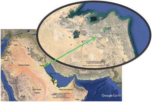
The location is centered between two major highways (5th and 6th Ring Highways) in a concentrated mixed commercial/residential area and north of the Kuwait International Airport. While not near the heavy refineries and industries in southern Kuwait, the site is impacted by land–sea breezes that recirculate emitted pollutants from throughout the Persian Gulf (Freeman et al., 2017a). A data set from December 1, 2012, to September 30, 2014, was used for this study. Parameters available are shown in Table 3.

Table 3. Chemical and meteorological parameters captured at the Air Monitoring Station.

Chemical analytes	Meteorological
Nitrous oxide (NO)	Wind direction (WD)
Ammonia (NH3)	Wind speed (WS)
Ozone (O3)	Temperature
Sulfur dioxide (SO2)	Atmospheric pressure (ATP)
Formaldehyde (CH2O)	Solar radiation (SR)
Nitrogen dioxide (NO2)	Relative humidity (RH)
Benzene (C6H6)
Toluene (C7H8)
p-Xylene (C8H10)
m Xylene (C8H10)
1,2,3-trimethylbenzene (C6H3(CH3)3)
o-Xylene (C8H10)
Ethylene glycol tertiary butyl ether (ETB) (C6H14O2)
Styrene (C8H8)
Chlorine (Cl2)
Carbon dioxide (CO2)
Methane (CH4)
Hydrogen sulfide (H2S)
Carbon monoxide (CO)

The local O₃ air quality standard is 75 ppb measured against an 8-hr moving average (KEPA 2017). The DOAS station recorded O₃ concentrations hourly, along with the other measured parameters. Measured units (μg/m³) were converted to ppb using the conversion formula

(9)

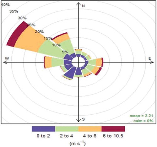
where C(ppb) is the gas concentration in parts per billion, C(μg/m³) is the concentration in micrograms per cubic meter, R is the ideal gas constant given as 8.3144 m³ kPa K⁻¹ mol⁻¹, MW is the molecular weight of the gas in grams per mole (O₃ = 48.01 g/mole), T is the ambient temperature in degrees Kelvin, and P is the atmospheric pressure at ground level (kPa). The station receives a prevailing wind from the northwest throughout the year, as shown in Figure 7.

Figure 7. Station wind rose from 2012 to 2014.

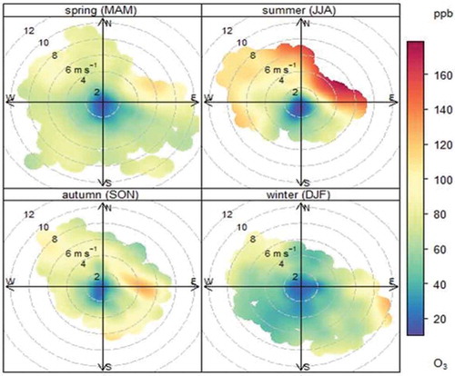
Seasonal effects are shown in a bivariate polar plot in Figure 8. High O₃ concentrations occur in the summer months from June to August, but come from the northeast, indicating the transport of pollutants from the coast. Not surprisingly, most of the compliance exceedances take place during this period.

Figure 8. Seasonal bivariate polar plots of 1-hr O_3.

Average hourly O₃ and NOx concentrations are shown in Figure 9. The two variables are highly inverse correlated (R² = −0.963), with common maxima/minima at 3:00 a.m., 6:00 a.m., 2:00 p.m., and 10:00 p.m. The raw hourly data are less correlated (R² = –.576), but still higher than other variables. The NOx peaks correspond to rush-hour traffic periods with winds blowing from the 6th and 7th Ring Highways in the southwest. O₃ levels peak in the afternoon, corresponding with solar radiation levels, but there is also a local maximum, or “morning bump,” due to photolyzed chlorine ions reacting with N₂O₅ to form NO₃ as part of the O₃ formation cycle in eq 2 (Calvert et al. 2015). The formation of NO₃ radicals was observed to be inversely related to O₃ concentrations (Song et al. 2011).

Figure 9. Hourly averages of 1-hr O₃ and NOx.

Building the RNN

The RNN used in this study used the Keras (version 2.0.9) machine learning application programming interface (Chollet et al., 2015) with Theano back end. Theano is a C++ library that allows mathematical expressions to be calculated symbolically and evaluated using data sets in matrices and arrays (Al-Rfou et al. 2016). The architecture used a single RNN layer with LSTM and a single output feed forward node. The output activation function for both layers was the sigmoid function, while the activation function for the recurrent nodes was the tanh function. The learning rate, α, was left at the default value of 0.002 (Chollet et al., 2015). Other Keras defaults included weight initialization (using a uniform distribution randomizer). Regulation was not used, although a dropout layer was included between the LSTM and the output layer.

Input data preparation

Each available feature was compared to the maximum possible data range of 16,056 hourly measurements over the observation period. Gaps in data were assumed to be Missing completely at random (MCAR) and attributed to maintenance down-time, power failures, and storm-related contamination (Le, Batterman, and Wahl 2007). Additionally, some data were out of range or had negative readings (Junger and Ponce De Leon 2015). Data recorded as a 0 were assumed to be censored and converted to the smallest recorded value within the data set of the individual parameter (Raa, Aneiros, and Vilar 2015). Negative and missing data were converted to 0 and identified using a filter mask. Two different single imputation (SI) techniques were used based on the number of consecutive gaps in data. For gaps (g) < 8, the first measurement and last measurement within the gap were used as a Bayesian estimator based on the previous observation to create a linear estimate of the missing data given by

(10)

where n is the missing data point in sequence (), and

(11)

For consecutive gaps > 8, the corresponding hourly measurement from the previous and preceding day was averaged:

(12)

The value of eight consecutive gaps was determined by comparing the root mean square error (RMSE) of the original data with data generated from the different statistical (imputed data) methods on artificially generated gaps (Junninen et al. 2004). The first method’s error varied with gap size, while the second method had a higher, static error. The RMSE for O₃ and NOx using the first method is shown in Figure 10 along with the intersection of the second method.

Figure 10. RMSE of O₃ and NOx from consecutive gaps of data using the first imputation method.

Features with more than 50% missing data, like RH and chlorine (Cl₂), were discarded. The remaining variables from Table 3 had few missing data points, ranging from 41 missing points out of 16,053 (0.3%) for WS, WD, and temperature, to 137 missing points (0.9%) for NH₃. The available data set used for this study is larger than data sets used in other studies that had up to 16% missing data (Taspnar 2015). Missing data adds noise to the training set and are often used to improve generalization and prevent overfitting the network to meet the training data set. Adding dropouts, or intentional data removal, is often used during network training for this reason (Srivastava et al. 2014).

Cyclic and continuous data

WD and time of day were converted into representations that preserved their cyclic nature. Wind direction was converted into sine and cosine components (Arhami, Kamali, and Rajabi 2013). Other parameters were transformed and scaled between values of 0 and 1 (Chatterjee et al. 2017) using the MinMaxScaler function in the Python Sci-Kit preprocessor library (Pedregosa et al. 2011). Overall, 25 features were prepared for initial training. These included the parameters measured in Table 3 with the addition of sine and cosine components for wind direction.

Feature selection using decision trees

Prior to training the RNN, features were reviewed to reduce input dimensionality by training multiple decision trees on the data sets and prioritizing features using the feature importance metric calculated during classifier training with the DecisionTreeClassifier, also in the Sci-Kit library (Pedregosa et al. 2011). Decision trees and random forest classifiers have been used to reduce input dimensions for sensors (Cho and Kurup 2011) and data classification competitions, outperforming other methods such as PCA and correlation filters (Al-Alawi, Abdul-Wahab, and Bakheit 2008; Silipo et al. 2014; Voukantsis et al. 2011). Decision trees are a supervised learning algorithm that recursively partition inputs into non-overlapping regions based on simple prediction models (Loh 2011; Singh, Gupta, and Rai 2013). Decision trees do not require intensive resources to train and evaluate, and keep their features, unlike PCA that transforms input variables into linear combinations based on the singular value decomposition (SVD) of the total data set’s covariance matrix (Wang, Ma, and Joyce 2016). While PCA is a form of unsupervised learning that allows dimensionality reduction by removing the number of transformed components fed to the input, decision trees identify which raw variables offer less impact so that they can be removed from the data collection stream. This can reduce future efforts required to collect, clean, and prepare data sets.

Using PCA for model input also limits the inclusion of new data that may become available on real-time systems. If a model is trained on transformed principal components only, any new data must also be transformed, thus changing the historical data set. Using a linear transformation method that only changes the individual observation and not the entire data set is more practical for time-series applications where new data is expected to be added over time. Other feature reduction techniques include evaluating contribution factors of weights to nodes to remove, or “prune,” low-value weights (de Oña and Garrida, 2014). This technique is not recommended for RNNs, especially with LSTMs, because of the way the weights are updated through different time steps. Alternative pruning techniques can be applied to RNNs to not only reduce inputs, but also reduce internal interconnections between the LSTM and look-back nodes (Narang et al. 2017). We did not explore internal pruning techniques in this paper. Instead, we evaluated the contribution of features externally and independent of the RNN using decision trees. Binary classification trees, a type of decision tree used for categorical separation, were trained to predict exceedances of 8-hr ave O₃ over 1-hr to 12-hr horizons. Individual observations were first scaled using the MinMaxScaler function based on the equation

(13)

where x_max and x_min are the maximum and minimum values in the data set, respectively. It can be argued that this method also suffers from legacy biasing like PCA in that the system retains x_max and x_min in order to restore transformed data to original scale, similar to a key for encryption decoding. If new data are included that exceed the x_max/x_min values, the data need to be reprocessed using the new points. Since we are already working with a historical data set and not using real-time data, there is no need to incorporate this issue. However, even if we were using real-time data, we could safely assume that any value measured that exceeded x_max in our historical set was also an extreme point and could be accounted for in the model as a value > 1.

Eighty percent (80%) of the scaled data were divided into a training set, with 20% reserved for testing. In larger data sets, a percentage of the total data is often reserved to allow parameter optimization prior to training in order to reduce time and system resources. Additionally, for FFNNs, training often takes hundreds or thousands of epochs, where an epoch is a complete training cycle that uses all training sets. With our relatively small data set and fast training using the LSTM, reviewing system performance using the full training set did not take much time and therefore did not require reserving a subset.

Output exceedances were classified by the decision tree as either 0 (less than the exceedance standard of 75 ppb) or 1 (exceeds the standard). Overall accuracy of each horizon was measured using the accuracy score function in Sci-Kit, which calculated the standard error of exact matches of the observed output with the predicted (Raschka 2016). Other classifiers in the Sci-Kit library were evaluated as well, including SVMs and Random Forest classifiers. The decision tree in classification mode using “gini” criteria to measure the data split at each decision node proved to be the most accurate. The importance of each feature was computed using the Sci-Kit feature_importances_ function that normalizes the total reduction of the criterion brought by individual features. Results of individual feature importance from classifying O₃ exceedances at different horizons are shown in Figure 11. The computed values are unitless and displayed in relative importance to each other.

Figure 11. Feature importance from decision tree prediction of 8-hr O₃ exceedances from 1 hr to 12 hr.

Output data preparation

The RNN output was trained to predict the 8-hr moving average of measured 1-hr O₃. To predict future values, the calculated values were shifted in time based on the desired horizon so that input observations X (t = 0) was trained on Y (t = 12) if the prediction horizon was 12 hr. Output data were generated from 8-hr moving averaged O₃ calculated from measured 1-hr O₃ concentrations at each station. The first 7 hours of both the input and output training data set was then discarded.

Tensor preparation for RNN input data

Data sets provided to the RNN were converted into three-dimensional tensors based on the sample size of data. The sample size was based on the number of look-back elements within the RNN, as compared to an observation that represented one row of the original data set, X. The transformation of the original two-dimensional data set X is illustrated in Figure 12 using Python notations. Assuming X is a data set of input data (for training or testing the RNN) with n observations and p variables, the total number of elements is the product of n and p, or 20 elements for the 5 × 4 data set in the figure. A tensor (T) is created with dimension (s, l, p) where s is the number of samples, given as n – l. The total number of elements within T is s – l – p. In the example of Figure 12, the dimensions of T are s = 5 – 2 = 3, l = 2, and p = 4.

Figure 12. Process of converting data input columns into a tensor for training the RNN.

Analysis of results

Final parameter selection

Because of the Tensor formation for input, the actual number of samples provided for training and testing was based on the look-ahead horizon and number of recurrent (look-back) units of the individual run. The farther out the prediction, the fewer samples were available because of the time shifting required. The total amount of samples available for training and testing could be calculated as total samples = (16,035 – h) where h is the prediction horizon (as an integer value > 1). The number of training epochs was limited after reviewing training error values up to 20 epochs for look-ahead horizons of 24 hr, 36 hr, and 48 hr as seen in Figure 13. An optimum number of 10 epochs was used for later model runs, as it minimizes the training error without overfitting, which begins to take place after 12 epochs, especially in Figure 13a.

Figure 13. Loss function errors for training and test data sets for different horizons at (a) 24 hr, (b) 36 hr, and (c) 48 hr.

Performance measures

Final parameter selection and performance were measured by mean absolute error (MAE) and root mean square error (RMSE). MAE and RMSE are widely used measures of continuous variables, with RMSE criticized for overbiasing toward large errors (Chai and Draxler 2014; Willmott and Matsuura 2005). Both metrics were calculated for comparison; however, MAE is used more often for descriptive analytics in this paper.

Impact of features and parameters on results

The network trained very well with all 25 input features from Table 3. An example of the predicted results compared with the observed measurements (8-hr ave O₃) over a 24-hr horizon is shown in Figure 14.

Figure 14. Results of training an RNN with a 24-hr horizon.

The MAE for this scenario is 0.41 ppb during training and 0.37 ppb during testing. The residuals of this scenario are shown in Figure 15, where they show a Normal distribution tendency (skewness = 0.411, kurtosis = 3.94, where Normal is 0 and 3, respectively) with a positive bias given by the distribution mean of 1.632 ppb. This is consistent with Figure 14, which shows the model slightly underpredicting.

Figure 15. Distribution of residual test errors for 24-hr horizon network.

The results of the decision tree analysis in Figure 11 showed that many features could be removed without impacting network performance. Features were removed based on the order of least importance in groups of five until the most prominent feature remained. The results in Figure 16 show that overall training error improves with fewer inputs. By removing input features, the system complexity is also reduced, allowing the network to train easier. While providing better training results, reducing feature inputs also makes it easier to overfit on the training data.

Figure 16. Training error associated with feature reduction on network prediction.

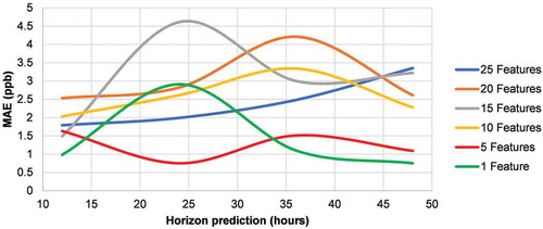
Based on the training error curves in Figure 16, the five-feature data set was used for evaluation because it provided stable errors over the prediction horizons of interest. The features used were (in order of importance) 8-hr ave O₃ in ppb, 1-hr O₃ in ppb, SR, the cosine of WD, and CH₄. Parameter sensitivity analysis was performed on a model with default values shown in Table 4.

Table 4. Default values for parameter sensitivity analysis.

Parameter	Default value
Input features	26
Prediction horizon (hr)	24
Look back nodes	26
Samples/batch	72
Dropout factor	0.2

All other parameters were held constant as an individual parameter was varied. The prediction horizon value of 24 hr was held constant throughout all runs, shown in Figure 17. In all cases, the error measurements, MAE and RMSE, showed similar forms, despite the RMSE having a consistently higher value, as expected, and as seen in other research (Singh et al. 2012). The prediction horizon of the model using the five-feature data set is shown in Figure 17.

Figure 17. Prediction horizons using five features and default parameters.

As the prediction extends further into the future (>80 hr), the training error climbs rapidly, while the test error appears to level off. The model began to overfit by this point and predictions past that range were considered to be unreliable. The results in Figure 18a show training error for different prediction horizons over several parameters. The parameter that influences the model performance the most is the number of look-back nodes in relation to the prediction horizon. A horizon value of +2 provides the lowest errors, while adding additional nodes increases the model complexity and makes training more challenging. Samples/batches in Figure 18b show relatively little error variance until many samples are included (>75 samples/batch). While more samples per batch are preferred to reduce training time, too many create bias in the loss function as the overall average of each sample reduces chances for updates. The number of recurrent, or look-back, nodes in relation to the prediction horizon was considered in Figure 18b. Both training and test results are minimized at 26, the horizon value + 2. This was consistent with other horizon prediction values such as 36 and 48. As more look-back nodes are added, the error increases. Finally, the use of dropout is recommended to improve generalization of the model and reduce overfitting (Gal and Ghahramani 2016). For this model, dropout was applied only between the output of the LSTM layer and the FF output layer. The error shows reasonably good optimization at around 0.2. The errors level out at higher rates at around 0.35. The default values were the optimum parameters based on the results shown in Figure 18.

Figure 18. Impact of (a) batch samples, (b) look-back nodes, and (c) dropout factor parameters on training errors in the model.

An LSTM model has many more variables that can be optimized compared to other models. The RNN used in this study with 25 input features had 16,485 updateable parameters, of which 16,432 were in the LSTM layer alone. As a comparison, an FFNN with 3 hidden layers (5 layers total), bias on all layers, and the same 25 feature inputs had only 2,107 parameters. Nonlinearities are further introduced during the training phase, in which the derivative of the activation function for each layer is used to influence the weight updates. It is therefore difficult to fully explain the mechanisms driving the output results of complex DL models. In order to ensure the model is working, the output must be compared with known results and parameters adjusted to optimize performance.

Comparison to previous studies

Previous studies mentioned in the first section used RMSE and error measurement methods other than MAE. The three studies that used RMSE were compared to our results with an LSTM network. Luna et al. (2014) used SVMs and FFNNs. Feng et al. (2011) used a multilayered system that included an SVM and a genetic algorithm-stabilized FFNN. Wang and Lu used an FFNN with a particle swarm optimization (Wang and Lu 2006). All studies, except Gomez et al. (2003), used PCA to preprocess the data. Comparing the results of the RNN to these previous studies gives an initial impression that the RNN has an order of magnitude improvement over the best FFNN or SVM models, as shown in Table 5.

Table 5. Comparison of RNN test data results to previously published results.

Source	Prediction horizon	Results (RMSE)	RNN (RMSE)
Luna et al. (2014)	1 hr	6.3–12.3	0.8
Feng et al. (2011)	12 hr	5.5–86.9	1.5
Wang and Lu (2006)	24 hr	7.9–11.2	2.5
Gomez et al. (2003)	24 hr	6.9–9.9

The results cannot, however, be directly compared because they were based on different data sets. While the other studies used complex and hybrid architectures along with complicated preprocessing, the RNN model preprocessing was very simple after the features were prioritized using a decision tree. The RNN and LSTM are themselves complex algorithms with many internal parameters that undergo training and updates.

Comparison to different models

The RNN model performance was compared to other forecasting models using the same dataset by comparing 24 hr predictions against an FFNN with three hidden layers and an ARIMA model. The FFNN was built with the Keras library using relu activation functions in the hidden layers and sigmoid function for the output. The inputs included all the parameters from Table 3 and the model was allowed to train for 1,000 epochs. The number of nodes in the hidden layer was based on the estimated number of hidden nodes = (SF × number of input nodes) + number of output nodes, where SF is a scaling factor between 0.5 and 1 (Papaleonidas and Iliadis 2013). For an SF of 0.75, the number of nodes is 20 nodes in each hidden layer. An MSE loss function and Nadam optimizer were also used to build the model. The ARIMA model was built using the arima function in R and fitted on the 8-hr ave O₃ only. The formatting parameters p, d, and q were automatically estimated using the auto.arima function as 3, 0, and 0, respectively (Hyndman and Athanasopolous, 2013). The results are shown in Figure 19 and summarized in Table 6.

Table 6. Comparison of different forecasting errors over a 24-hr period.

	RNN	FFNN	ARIMA
MAE (ppb)	0.235	15.28	23.574

Figure 19. Comparison of different model forecasts over a 24-hr period.

Conclusion and recommendations

This is one of the first papers that employ deep learning techniques in the prediction of air quality time series events. This new methodology produced very good results using our validation data set. A recurrent neural network with LSTM was trained on time series air pollutant and weather data from an air monitoring station in Kuwait to predict 8-hr ave O₃ over different prediction horizons. Missing data and censored data were replaced using a first-order imputation technique that accounted for sequential influence of previous readings for small gaps (<8 consecutive gaps) and seasonal effects for larger gaps. A decision tree was used to prioritize the most influential features for training by categorizing pollution exceedances using the input parameters.

Prioritizing and removing less important feature allows for real-time observations to be fed into the model without transforming large blocks of data as is required when using principal components or wavelets. New observations need only be scaled by normalizing or standardizing with the scaling values calculated from historical data sets.

A sensitivity analysis of key parameters showed that the network could be tuned for optimal performance. Measurements of the performance, in terms of observed and predicted results, were consistent in form, but the RMSE was always biased higher than the MAE measurement. Either measurement would have produced the same conclusions based on observation of local minima and maxima regardless of the error value. Error increased with the complexity of the network, even with reduced features. This “curse of dimensionality” led to overfitting of the model, reducing the ability to generalize if new data sets were introduced. Slight overfitting is not a problem for time-series data that follow predictable cyclic patterns and if the main output product of interest goes higher than a set limit.

While the results cannot be directly compared to other studies because different data sets were used, the results should not be dismissed either. Comparing the same data set results to other common forecasting models such as ARIMA and a multilayer FFNN shows that the RNN does perform significantly better. The complexity of RNN implementation has been dramatically reduced with the use of the Keras developmental library, allowing non-computer scientists the ability to use DL without the coding overhead. The LSTM model provided very good results for this case and can be applied to other environmental time-series challenges such as forecasting wide-area pollution exceedances from multiple stations and multiple pollutants. LSTMs could also be effective in predicting individual source emissions or modeling source apportionment under different criteria.

Reducing features and optimizing parameters assisted with lowering error of both training and test sets. Initial runs using local data showed excellent results compared to the performance from FFNNs, even with the inclusion of complex preprocessing of input data and architecture of the model. The relative ease of model structure in the programming code is misleading, though. The Keras and Theano libraries are some of the most advanced, validated, and complex libraries available in the research community. The underlying errors within the model implementation may not be resolved or even quantified. However, they are still useful tools for rapid prototyping and architecture validation. Using the data sets of the sources listed in Table 5 with our RNN would be a more direct way to prove which method works better. Further investigations will target multiple station influences on local concentration prediction, as well as how imputation techniques for missing data impacts overall prediction accuracy.

Acknowledgment

Data collection was completed under the United Nations Development Program (UNDP) Kuwait Integrated Environmental Management System project from 2010 to 2015.

Additional information

Funding

We acknowledge partial financial support of Natural Science and Engineering Research Council of Canada (NSERC) and Lakes Environmental.

Notes on contributors

Brian S. Freeman

Brian S. Freeman is a Ph.D. candidate in the School of Engineering at the University of Guelph, Ontario, Canada.

Graham Taylor

Graham Taylor is an associate professor at the School of Engineering at the University of Guelph, Ontario, Canada.

Bahram Gharabaghi

Bahram Gharabaghi is a professor at the School of Engineering at the University of Guelph, Ontario, Canada.

Jesse Thé

Jesse Thé is the president of Lakes Environmental Software at Waterloo, Ontario, Canada.

References

- Abadi, M., A. Agarwal, P. Barham, E. Brevdo, Z. Chen, C. Citro, G.S. Corrado, A. Davis, J. Dean, M. Devin, S. Ghemawat, I. Goodfellow, A. Harp, G. Irving, M. Isard, Y. Jia, R. Jozefowicz, L. Kaiser, M. Kudlur, J. Levenberg, D. Mané, R. Monga, S. Moore, D. Murray, C. Olah, M. Schuster, J. Shlens, B. Steiner, I. Sutskever, K. Talwar, P. Tucker, V. Vanhoucke, V. Vasudevan, F. Viégas, O. Vinyals, P. Warden, M. Wattenberg, M. Wicke, Y. Yu, and X. Zheng (2015) TensorFlow: Large-scale machine learning on heterogeneous systems. tensorflow.org (accessed January 16, 2018).
- Abdul-Wahab, S.A. 2001. IER photochemical smog evaluation and forecasting of short-term ozone pollution levels with artificial neural networks. Process Saf. Environ. Prot. 79 (2):117–128. doi:10.1205/09575820151095201.
- Achcar, J.A., E.R. Rodrigues, and G. Tzintzun. 2011. Modeling the time between ozone exceedances. Braz. J. Probab. Stat. 25 (2):183–204. doi:10.1214/10-BJPS116.
- Al-Alawi, S.M., S.A. Abdul-Wahab, and C.S. Bakheit. 2008. Combining principal component regression and artificial neural networks for more accurate predictions of ground-level ozone. Environ. Modell. Software 23 (4):396–403. doi:10.1016/j.envsoft.2006.08.007.
- Al-Rfou, R., G. Alain, A. Almahairi, C. Angermueller, D. Bahdanau, N. Ballas, F. Bastien, J. Bayer, A. Belikov, A. Belopolsky, et al. 2016, May. Theano: A Python framework for fast computation of mathematical expressions. arXiv e-prints abs/1605.02688.
- Amann, M., D. Derwent, B. Forsberg, O. Hnninen, F. Hurley, M. Krzyzanowski, F.D. Leeuw, S.J. Liu, C. Mandin, J. Schneider, P. Schwarze, and D. Simpson (2008). Health risks of ozone from long-range transboundary air pollution. Report, WHO Regional Office for Europe. http://www.euro.who.int/__data/assets/pdf_file/0005/78647/E91843.pdf (accessed January 17, 2018).
- Arhami, M., N. Kamali, and M.M. Rajabi. 2013. Predicting hourly air pollutant levels using artificial neural networks coupled with uncertainty analysis by Monte Carlo simulations. Environ. Sci. Pollut. Res. 20 (7):4777–4789. doi:10.1007/s11356-012-1451-6.
- Beck, J., M. Krzyzanowski, and B. Koffi (1998). Tropospheric ozone in the European Union: The consolidated report. Report, European Environment Agency. https://publications.europa.eu/en/publication-detail/-/publication/3cacc7e4-1113-44e4-810d-ac630234fd76 (accessed January 17, 2018).
- Bei, N., G. Li, Z. Meng, Y. Weng, M. Zavala, and L. Molina. 2014. Impacts of using an ensemble Kalman filter on air quality simulations along the California-Mexico border region during Cal-Mex 2010 field campaign. Sci. Total Environ. 499 (Supplement C):141–153. doi:10.1016/j.scitotenv.2014.07.121.
- Bengio, Y. (2012). Practical recommendations for gradient-based training of deep architectures. CoRR 1206.5533. http://arxiv.org/abs/1206.5533.
- Biancofiore, F., M. Busilacchio, M. Verdecchia, B. Tomassetti, E. Aruffo, S. Bianco, S. Di Tommaso, C. Colangeli, G. Rosatelli, and P. Di Carlo. 2017. Recursive neural network model for analysis and forecast of PM10 and PM2:5. Atmos. Pollut. Res. 8 (4):652–659. doi:10.1016/j.apr.2016.12.014.
- Biancofiore, F., M. Verdecchia, P. Di Carlo, B. Tomassetti, E. Aruffo, M. Busilacchio, S. Bianco, S. Di Tommaso, and C. Colangeli. 2015. Analysis of surface ozone using a recurrent neural network. Sci. Total Environ. 514:379–387. doi:10.1016/j.scitotenv.2015.01.106.
- Brown, S. S., and J. Stutz. 2012. Nighttime radical observations and chemistry. Chem. Soc. Rev. 41 (19):6405–6447. doi:10.1039/C2CS35181A.
- Calvert, J., J. Orlando, W. Stockwell, and T. Wallington. 2015. The mechanisms of reactions influencing atmospheric ozone. New York, NY: Oxford University Press. ISBN: 978-0-19-023302-0.
- Central Intelligence Agency (2015). CIA World Factbook: Middle East: Kuwait. https://www.cia.gov/library/publications/the-world-factbook/geos/ku.html. (accessed January 26, 2018)
- Chai, T., and R.R. Draxler. 2014. Root mean square error (RMSE) or mean absolute error (MAE)?-Arguments against avoiding RMSE in the literature. Geosci. Model Dev. doi:10.5194/gmd-7-1247-2014.
- Chatterjee, S. K., S. Das, K. Maharatna, E. Masi, L. Santopolo, I. Colzi, S. Mancuso, and A. Vitaletti. 2017. Comparison of decision tree based classification strategies to detect external chemical stimuli from raw and filtered plant electrical response. Sens. Actuators, B 249 (Supplement C):278–295. doi:10.1016/j.snb.2017.04.071.
- Che, Z., S. Purushotham, K. Cho, D. Sontag, and Y. Liu (2016). Recurrent neural networks for multivariate time series with missing values. CoRR abs/1606.01865. http://arxiv.org/abs/1606.01865.
- Cho, J.H., and P.U. Kurup. 2011. Decision tree approach for classification and dimensionality reduction of electronic nose data. Sens. Actuators, B 160 (1):542–548. doi:10.1016/j.snb.2011.08.027.
- Chollet, F. et al. 2015. Keras: Deep learning library for Theano and Tensor ow. github.com/fchollet/keras. http://github.com/fchollet/keras.(accessed February 12, 2018).
- Cooper, O.R., A. Stohl, M. Trainer, A.M. Thompson, J.C. Witte, S.J. Oltmans, G. Morris, K. E. Pickering, J.H. Crawford, G. Chen, R.C. Cohen, T.H. Bertram, P. Wooldridge, A. Perring, W.H. Brune, J. Merrill, J.L. Moody, D. Tarasick, P. Ndlec, G. Forbes, M.J. Newchurch, F.J. Schmidlin, B.J. Johnson, S. Turquety, S.L. Baughcum, X. Ren, F.C. Fehsenfeld, J.F. Meagher, N. Spichtinger, C. C. Brown, S.A. Mc-Keen, I.S. McDermid, and T. Leblanc. 2006. Large upper tropospheric ozone enhancements above midlatitude North America during summer: In situ evidence from the IONS and MOZAIC ozone measurement network. Journal of Geophysical Research: Atmospheres 111 (D24). doi:10.1029/2006JD007306.
- Crosman, E.T., and J.D. Horel. 2010. Sea and lake breezes: A review of numerical studies. Boundary Layer Meteorol. 137 (1):1–29. doi:10.1007/s10546-010-9517-9.
- CSB (2016). Chapter 3 population. Report, State of Kuwait Central Statistic Bureau. https://www.csb.gov.kw/Socan_Statistic_EN.aspx?ID=67.(accessed February 12, 2018).
- Cuxart, J., M.A. Jimnez, M.T. Prtenjak, and B. Grisogono. 2014. Study of a sea-breeze case through momentum, temperature, and turbulence budgets. J. Appl. Meteorol. Climatol. 53 (11):2589–2609. doi:10.1175/JAMC-D-14-0007.1.
- de Oña, J., and C. Garrido. 2014. Extracting the contribution of independent variables in neural network models: A new approach to handle instability. Neural Comput. Appl. 25 (3):859–869. doi:10.1007/s00521-014-1573-5.
- Dozat, T. (2016). Incorporating Nesterov momentum into ADAM. In 4th International Conference on Learning Representations. https://openreview.net/pdf?id=OM0jvwB8jIp57ZJjtNEZ.(accessed February 12, 2018).
- Duchi, J., E. Hazan, and Y. Singer. 2011. Adaptive subgradient methods for online learning and stochastic optimization. J. Mach. Learn. Res. 12:2121–2159. http://dl.acm.org/citation.cfm?id=1953048.2021068.
- Elangasinghe, M.A., N. Singhal, K.N. Dirks, J.A. Salmond, and S. Samarasinghe. 2014. Complex time series analysis of PM10 and PM2:5 for a coastal site using artificial neural network modelling and k-means clustering. Atmos. Environ. 94:106–116. doi:10.1016/j.atmosenv.2014.04.051.
- Ettouney, R.S., F.S. Mjalli, J.G. Zaki, M.A. ElRifai, and H.M. Ettouney. 2009. Forecasting of ozone pollution using artificial neural networks. Manage. Environ. Qual. Int. J. 20 (6):668–683. doi:10.1108/14777830910990843.
- Fan, J., Q. Li, J. Hou, X. Feng, H. Karimian, and S. Lin (2017). A spatiotemporal prediction framework for air pollution based on deep RNN. In 2nd International Symposium on Spatiotemporal Computing, Volume V-4/W2, pp. 15–22. ISPRS Annals of the Photogrammetry, Remote Sensing and Spatial Information Sciences. DOI:10.5194/isprs-annals-IV-4-W2-15-2017.
- Feng, Y., W. Zhang, D. Sun, and L. Zhang. 2011. Ozone concentration forecast method based on genetic algorithm optimized back propagation neural networks and support vector machine data classification. Atmos. Environ. 45 (11):1979–1985. doi:10.1016/j.atmosenv.2011.01.022.
- Finlayson-Pitts, B., and J.J.N. Pitts. 1993. Atmospheric chemistry of tropospheric ozone formation: Scientific and regulatory implications. Air Waste 43 (8):1091–2100. doi:10.1080/1073161X.1993.10467187.
- Freeman, B., B. Gharabaghi, J. Thé, M. Munshed, S. Faisal, M. Abdullah, and A.A. Aseed. 2017a. Mapping air quality zones for coastal urban centers. J. Air Waste Manage. Assoc. 67 (5):565–581. doi:10.1080/10962247.2016.1265025.
- Freeman, B., E. McBean, B. Gharabaghi, and J. Thé. 2017b. Evaluation of air quality zone classification methods based on ambient air concentration exposure. J. Air Waste Manage. Assoc. 67 (5):550–564. doi:10.1080/10962247.2016.1263585.
- Gal, Y., and Z. Ghahramani 2016. A theoretically grounded application of dropout in recurrent neural networks. ArXiv e-prints 1512.05287. https://arxiv.org/abs/1512.05287v5.
- Gardner, M.W., and S.R. Dorling. 1998. Artificial neural networks (the multilayer perceptron) A review of applications in the atmospheric sciences. Atmos. Environ. 32 (1415):2627–2636. doi:10.1016/S1352-2310(97)00447-0.
- Gheyas, I.A., and L.S. Smith. 2011. A novel neural network ensemble architecture for time series forecasting. Neurocomputing 74 (18):3855–3864. doi:10.1016/j.neucom.2011.08.005.
- Glavas, S.D., and E. Sazakli. 2011. Ozone long-range transport in the Balkans. Atmos. Environ. 45 (8):1615–1626. doi:10.1016/j.atmosenv.2010.11.030.
- Gomez, P., Nebot, Angela, Ribeiro, Sabrine, Alquézar, René, Mugica, Francisco,Wotawa and Franz. 2003. Local maximum ozone concentration prediction using soft computing methodologies. Syst. Anal. Modell. Simul. 43 (8):1011–1031. doi:10.1080/0232929031000081244.
- Goodfellow, I., Y. Bengio, and A. Courville. 2016. Deep Learning. Cambridge, MA: MIT Press. ISBN: 9780262035613.
- Graves, A. (2013). Generating sequences with recurrent neural networks. CoRR abs/1308.0850. http://arxiv.org/abs/1308.0850.
- Graves, A., A. Mohamed, and G.E. Hinton 2013. Speech recognition with deep recurrent neural networks. CoRR abs/1303.5778. http://arxiv.org/abs/1303.5778.
- Hinton, G.E., and S. Osindero. 2006, July. A fast learning algorithm for deep belief nets. Neural Comput. 18(7):1527–1554. doi:10.1162/neco.2006.18.7.1527.
- Hochreiter, S., and J. Schmidhuber. 1997. Long short-term memory. Neural Comput. 9 (8):1735–1780. doi:10.1162/neco.1997.9.8.1735.
- Hyndman, R., and G. Athanasopoulos. 2013. Forecasting: Principles and practice, Chapter 8.7 ARIMA modelling in R. Melbourne. Australia: OTexts.
- Junger, W.L., and A. Ponce De Leon. 2015. Imputation of missing data in time series for air pollutants. Atmos. Environ. 102:96–104. doi:10.1016/j.atmosenv.2014.11.049.
- Junninen, H., H. Niska, K. Tuppurainen, J. Ruuskanen, and M. Kolehmainen. 2004. Methods for imputation of missing values in air quality data sets. Atmos. Environ. 38 (18):2895–2907. doi:10.1016/j.atmosenv.2004.02.026.
- KAMCO 2013. State of Kuwait: Economic & financial facts. Report, KIPCO Asset Management Company KSC. http://www.kamconline.com/Temp/Reports/48218661-476e-43f1-8d12-ecc124e90e93.pdf.(accessed February 12, 2018).
- KEPA. 2017, June. Decree no. 8 of 2017 Promulgating the bylaws in accordance with the protection of external air against pollution. Kuwait: Kuwait Al Yom. 1345.
- Kingma, D.P., and J. Ba. 2014. Adam: A method for stochastic optimization. CoRR abs/1412.6980. http://arxiv.org/abs/1412.6980. (accessed February 18, 2018).
- Kuhlbusch, T.A.J., P. Quincey, G.W. Fuller, F. Kelly, I. Mudway, M. Viana, X. Querol, A. Alastuey, K. Katsouyanni, E. Weijers, A. Borowiak, R. Gehrig, C. Hueglin, P. Bruckmann, O. Favez, J. Sciare, B. Hoffmann, K. EspenYttri, K. Torseth, U. Sager, C. Asbach, and U. Quass. 2014. New directions: The future of European urban air quality monitoring. Atmos. Environ. 87:258–260. doi:10.1016/j.atmosenv.2014.01.012.
- Kurt, A., B. Gulbagci, F. Karaca, and O. Alagha. 2008. An online air pollution forecasting system using neural networks. Environ. Int. 34 (5):592–598. doi:10.1016/j.envint.2007.12.020.
- Le, H.Q., S.A. Batterman, and R.L. Wahl. 2007. Reproducibility and imputation of air toxics data. J. Environ. Monit. 9 (12):1358–1372. doi:10.1039/B709816B.
- Lelieveld, J., and F. Dentener. 2000. What controls tropospheric ozone? J. Geophys. Res. 105 (D3):3531–3551. doi:10.1029/1999JD901011.
- Liu, P.-W.G. 2007. Establishment of a Box-Jenkins multivariate timeseries model to simulate ground-level peak daily one-hour ozone concentrations at Ta-Liao in Taiwan. J. Air Waste Manage. Assoc. 57 (9):1078–1090. doi:10.3155/1047-3289.57.9.1078.
- Loh, W.-Y. 2011. Classification and regression trees. Data Min. Knowl. Discovery 1 (1):14–23. doi:10.1002/widm.8.
- Lu, W.Z., and W.J. Wang. 2005. Potential assessment of the support vector machine method in forecasting ambient air pollutant trends. Chemosphere 59 (5):693–701. doi:10.1016/j.chemosphere.2004.10.032.
- Luna, A.S., M.L.L. Paredes, G.C.G. de Oliveira, and S.M. Corra. 2014. Prediction of ozone concentration in tropospheric levels using artificial neural networks and support vector machine at Rio de Janeiro, Brazil. Atmos. Environ. 98:98–104. doi:10.1016/j.atmosenv.2014.08.060.
- Malley, C.S., D.K. Henze, J.C. Kuylenstierna, H.W. Vallack, Y. Davila, S.C. Anenberg, M.C. Turner, and M.R. Ashmore. 2017. Updated global estimates of respiratory mortality in adults >30 years of age attributable to long-term ozone exposure. Environ. Health Perspect. 125 (8). doi:10.1289/EHP1390.
- Narang, S., G. Diamos, S. Sengupta, and E. Elsen, 2017. Exploring sparsity in recurrent neural networks. CoRR abs/1704.05119. http://arxiv.org/abs/1704.05119.
- Nesterov, Y. 1983. A method of solving a convex programming problem with convergence rate O(1/k2). Sov. Math. Dokl. 27 (2):372–376. https://arxiv.org/pdf/1510.08740.pdf.
- Papaleonidas, A., and L. Iliadis. 2013. Neurocomputing techniques to dynamically forecast spatiotemporal air pollution data. Evolving Syst. 4 (4):221–233. doi:10.1007/s12530-013-9078-5.
- Pascanu, R., T. Mikolov, and Y. Bengio 2013. On the difficulty of training recurrent neural networks. In 30th International Conference on Machine Learning, Volume 28. W&CP., http://proceedings.mlr.press/v28/pascanu13.pdf.
- Pedregosa, F., G. Varoquaux, A. Gramfort, V. Michel, B. Thirion, O. Grisel, M. Blondel, P. Prettenhofer, R. Weiss, V. Dubourg, J. Vanderplas, A. Passos, D. Cournapeau, M. Brucher, M. Perrot, and E. Duchesnay. 2011, November. Scikit-learn: Machine learning in python. J. Mach. Learn. Res. 12:2825–230. http://dl.acm.org/citation.cfm?id=1953048.2078195.
- Prybutok, V.R., J. Yi, and D. Mitchell. 2000. Comparison of neural network models with ARIMA and regression models for prediction of Houston’s daily maximum ozone concentrations. Eur. J. Oper. Res. 122 (1):31–40. doi:10.1016/S0377-2217(99)00069-7.
- Raa, P., G. Aneiros, and J.M. Vilar. 2015. Detection of outliers in functional time series. Environmetrics 26 (3):178–191. doi:10.1002/env.2327.
- Raschka, S. 2016. Python machine learning. Birmingham UK: Packt Publishing. ISBN: 978-1-78355-513-0.
- Silipo, R., I. Adae, A. Hart, and M. Berthold 2014. Seven techniques for data dimensionality reduction. Report, KNIME.com AG. January 12, 2018).
- Singh, K.P., S. Gupta, A. Kumar, and S.P. Shukla. 2012. Linear and nonlinear modeling approaches for urban air quality prediction. Sci. Total Environ. 426 (Supplement C):244–255. doi:10.1016/j.scitotenv.2012.03.076.
- Singh, K.P., S. Gupta, and P. Rai. 2013. Identifying pollution sources and predicting urban air quality using ensemble learning methods. Atmos. Environ. 80 (Supplement C):426–437. doi:10.1016/j.atmosenv.2013.08.023.
- Song, F., J. Young Shin, R. Jusino Atresino, and Y. Gao. 2011. Relationships among the springtime ground level NOx, O3 and NO3 in the vicinity of highways in the US East Coast. Atmos. Pollut. Res. 2 (3):374–383. doi:10.5094/APR.2011.042.
- Srivastava, N., G. Hinton, A. Krizhevsky, I. Sutskever, and R. Salakhutdinov. 2014, January. Dropout: A simple way to prevent neural networks from overfitting. J. Mach. Learn. Res. 15 (1):1929–1958. http://dl.acm.org/citation.cfm?id=2627435.2670313.
- Sutskever, I., J. Martens, G. Dahl, and G. Hinton 2013. On the importance of initialization and momentum in deep learning. In Proceedings of the 30th International Conference on Machine Learning, Volume 28. http://www.datascienceassn.org/content/importanceinitialization-and-momentum-deep-learning. (accessed February 28, 2018).
- Tarasick, D., and R. Slater. 2008. Ozone in the troposphere: Measurements, climatology, budget, and trends. Atmos. Ocean 46 (1):93–115. doi:10.3137/ao.460105.
- Taspnar, F. 2015. Improving artificial neural network model predictions of daily average PM10 concentrations by applying principle component analysis and implementing seasonal models. J. Air Waste Manage. Assoc. 65 (7):800–809. doi:10.1080/10962247.2015.1019652.
- Theano Development Team 2016. Theano: A Python framework for fast computation of mathematical expressions. arXiv e-prints abs/1605.02688. http://arxiv.org/abs/1605.02688.
- Thornton Joel A., Kercher, James P., Riedel, Theran P., Wagner, Nicholas L., Cozic, Julie, Holloway, John S., Dube, William P., Wolfe, Glenn M., Quinn, Patricia K., Middlebrook, Ann M., Alexander, Becky, Brown, Steven S. 2010. A large atomic chlorine source inferred from mid continental reactive nitrogen chemistry. Nature 464: 271–274. doi: 10.1038/nature08905.
- Tieleman, T., and G. Hinton 2012. Lecture 6.5 - RMSprop: Divide the gradient by a running average of its recent magnitude. COURSERA: Neural Networks for Machine Learning, 4. http://www.cs.toronto.edu/~tijmen/csc321/slides/lecture_slides_lec6.pdf (accessed February 12, 2018).
- Vlachogianni, A., P. Kassomenos, A. Karppinen, S. Karakitsios, and J. Kukkonen. 2011. Evaluation of a multiple regression model for the forecasting of the concentrations of NOx and PM10 in Athens and Helsinki. Sci. Total Environ. 409 (8):1559–1571. doi:10.1016/j.scitotenv.2010.12.040.
- Voukantsis, D., K. Karatzas, J. Kukkonen, T. Rasanen, A. Karppinen, and M. Kolehmainen. 2011. Intercomparison of air quality data using principal component analysis, and forecasting of PM10 and PM2:5 concentrations using artificial neural networks, in Thessaloniki and Helsinki. Sci. Total Environ. 409 (7):1266–1276. doi:10.1016/j.scitotenv.2010.12.039.
- Walid, and Alamsyah. 2017. Recurrent neural network for forecasting time series with long memory pattern. J. Phys. Conf. Ser. 824 (1):012038. http://stacks.iop.org/1742-6596/824/i=1/a=012038.
- Wang, D., and W.-Z. Lu. 2006. Ground-level ozone prediction using multilayer perceptron trained with an innovative hybrid approach. Ecol. Modell. 198 (34):332–340. doi:10.1016/j.ecolmodel.2006.05.031.
- Wang, P., Y. Liu, Z. Qin, and G. Zhang. 2015. A novel hybrid forecasting model for PM10 and SO2 daily concentrations. Sci. Total Environ. 505 (Supplement C):1202–1212. doi:10.1016/j.scitotenv.2014.10.078.
- Wang, Y., X. Ma, and M.J. Joyce. 2016. Reducing sensor complexity for monitoring wind turbine performance using principal component analysis. Renew. Energy 97:444–456. doi:10.1016/j.renene.2016.06.006.
- Welch, E., X. Gu, and L. Kramer. 2005. The effects of ozone action day public advisories on train ridership in Chicago. Transp. Res. Part D: Transp. Environ. 10 (6):445–458. doi:10.1016/j.trd.2005.06.002.
- Willmott, C.J., and K. Matsuura. 2005. Advantages of the mean absolute error (MAE) over the root mean square error (RMSE) in assessing average model performance. Clim. Res. 30 (1):79–82. doi:10.3354/cr030079.
- Wirtz, D.S., M.G. El-Din, A.G. El-Din, and A. Idriss. 2005. Systematic development of an artificial neural network model for real-time prediction of ground-level ozone in Edmonton, Alberta, Canada. J. Air Waste Manage. Assoc. 55 (12):1847–1857. doi:10.1080/10473289.2005.10464780.
- Zickus, M., A.J. Greig, and M. Niranjan. 2002. Comparison of four machine learning methods for predicting PM10 concentrations in Helsinki, Finland. Water Air Soil Pollut. Focus 2 (5–6):717–729. doi:10.1023/A:1021321820639.