Integrating site-specific dispersion modeling into life cycle assessment, with a focus on inhalation risks in chemical production

ABSTRACT

It has become increasingly important for environmental managers to evaluate the human health (HH) impact of chemicals in their supply chain. Current life cycle assessment (LCA) methods are limited because they often only address the HH impact at large geographical scales. This paper aims to develop a method that derives a regionalized life cycle inventory data set and site-specific air dispersion modeling to evaluate the HH impact of chemicals along the life cycle phases at finer geographical scales to improve decision-making, with focus on inhalation pathway. More specifically, cancer risk and noncancer hazard index (HI) are quantified at the county level to identify high-risk regions and at the census tract level to reveal the geographical pattern of health impacts. The results showed that along the cradle-to-gate life cycle stages of a widely used chemical, methylene diphenyl diisocyanate (MDI), the accumulative inhalation risk was 3 orders of magnitude below the U.S. Environmental Protection Agency (EPA) risk management thresholds for both cancer risk (2.16 × 10⁻⁹) and noncancer HI (1.53 × 10⁻³). However, the absolute value of inhalation risks caused by the case study chemicals varied significantly in different geographical areas, up to 4 orders of magnitude. This paper demonstrates a feasible approach to improve human health impact assessment (HHIA) by combining site-specific air dispersion modeling and LCA using publicly available inventory data. This proposed method complements existing life cycle impact assessment (LCIA) models to improve HHIA by employing both HH risk assessment and LCA techniques. One potential outcome is to prioritize pollution prevention and risk reduction measures based on the risk maps derived from this method.

Implications: It has become increasingly important for environmental managers to evaluate the human health impacts of chemicals in their supply chain. Regionalized life cycle inventory data sets should be developed using publically available databases such as EPA’s toxic release inventory. The combination of site-specific dispersion modeling and life cycle assessment modeling can improve human health impact assessment of chemicals by providing more regionalized results along their supply chain.

Introduction

The chemical industry and chemical management regulations

In the United States, the chemical industry supported 25% of the gross domestic product (GDP) and produced 15% of the world’s chemicals in 2015 (American Chemistry Council 2016; Bureau of Economic Analysis 2016). According to the U.S. Environmental Protection Agency (EPA), there are currently over 84,000 chemicals listed in the Toxic Substances Control Act (TSCA) inventory (United States Government Accountability Office 2013). Federal and state agencies have set laws and regulations to manage hazard, exposure, and risks along a chemical’s supply chain. TSCA was passed in 1976 to evaluate hazards and potential risks from new or existing chemicals. In 1986, the Toxic Release Inventory (TRI) was created to address chemical releases from industrial facilities under the Emergency Planning and Community Right-to-Know Act. In 2016, the Frank R. Lautenberg Chemical Safety for the 21st Century Act was passed to strengthen the chemical management laws (United States Congress 2016). Under the strengthened chemical management law framework, the EPA has developed the ToxCast and ExpoCast programs to prioritize chemicals of concern (Biryol et al. 2017; Bonnell et al. 2018; Isaacs et al. 2014; Wambaugh et al. 2013, 2014). To achieve the goal of environmental and human health protection, many tools have been developed by federal agencies and academia to assess the impact of chemicals (Centers for Disease Control and Prevention 2012). For example, ExpoCast used two far-field tools: the USEtox model and the Risk Assessment IDentification and Ranking (RAIDAR) model, to prioritize chemical exposure among 1936 chemicals (Wambaugh et al. 2013). However, each existing tool has its strength and weakness.

Existing methods for evaluating human health impact of far-field chemical emissions

Human health risk assessment (HHRA) and life cycle assessment (LCA) are two methods that can be used to quantify chemical human health impact. HHRA is a receptor-based method that evaluates the human health impact of chemicals emitted to the environment for targeted population (e.g., a specific geographical location or an age group). HHRA often focuses on a chemical (e.g., is bisphenol A safe?). Since it is a receptor-driven method, HHRA is often conducted for individual life cycle phase separately. However, LCA considers the human health impacts from all life cycle emissions of a chemical simultaneously. Another key distinction between HHRA and LCA, subsequently described, is the risk minimization principle. HHRA is commonly referred as “only over the threshold” (Potting, Hauschild, and Wenzel 1999). It assumes that only the risks over certain thresholds (e.g., cancer risk: 1 in a million, noncancer hazard index (HI): 1) should be managed (EPA 2005).

LCA is another method for studying the environmental and human health impact of processes and products. Unlike HHRA, LCA defines a functional unit as the basis to collect the emission inventory released into the environment along life cycle phases, and in the life cycle impact assessment (LCIA) step, the toxic chemical emissions such as hazardous air pollutants (HAPs) are characterized according to human health end points, such as cancer and noncancer. Depending on the geographical scale of the LCIA models, human health impacts can be evaluated at global, continental, or regional levels. Some of the widely used LCIA models for human health impact assessment (HHIA) are listed in Table 1. The more recent model development focuses on providing more geographical relevance by quantifying regional environmental characteristics. For example, USEtox 2.0 provides regionalized environmental conditions for 24 regions in the world (Rosenbaum et al. 2011).

Table 1. Existing LCIA methods/models for assessing human health impact.

LCIA method/Human health characterization model	Last update to human health CFs	Level of regionalization
TRACI 2/USEtox (Bare 2011)	2016	USEtox divides the world into 24 regions* and provides regionalized environmental landscape parameters for each region.
CML/USEtox (Rosenbaum et al. 2008, Rosenbaum et al. 2011)	2010
ReCiPe/USES-LCA 2.0 (Zelm, Huijbregts, and Meent 2009)	2015	USES-LCA 2.0 provides default environmental landscape parameters at three geographical scales (global, continental, and urban). ReCiPe provides different CFs based on “archetype LCIA” such as high vs. low population density areas and high vs. very high stress watersheds.
IMPACT North America (Humbert et al. 2009)	2013	IMPACT North America divides the United States and Canada into 1° × 1° air cells, 523 watersheds, and five coastal zones. Within each cell or zone, the “archetype LCIA” is used to differentiate high vs. low population density area and high vs. low agricultural production regions.
GLOBOX (Wegener Sleeswijk and Heijungs 2010)	2011	GLOBOX divides the world into 250 regions and provides default environmental landscape parameters.

Notes. CF = characterization factor.

*With overlap (e.g., North America vs. USA and southern Canada).

Although HHIA in LCIA has been improved by regionalizing the environmental compartments, research efforts are still desirable to overcome two major obstacles in order to assess the health risk of chemicals along their life cycle phases. First, disaggregated life cycle inventory (LCI) data with site-specific geographical information are lacking. In current LCI databases such as Gabi and Ecoinvent (Thinkstep 2014; Weidema et al. 2013), the location of emissions is recorded at a large and often generic geographical scale, such as the continental air of North America, instead of a specific geographical coordinate. Except certain unit processes, most chemicals are produced in chemical plants that have geographical coordinates recorded in publicly available databases, such as EPA’s TRI and National Emissions Inventory (NEI). With the exact emission location, site-specific human health impact can be assessed for a unit process using localized meteorological, terrestrial, and demographical information. Second, current LCIA models assume that chemical distribution in each environmental compartment is homogenous. However, in a real-world scenario, chemical concentrations vary both temporally and geographically. For example, USEtox assumes that everyone in the entire continental compartment (a population of 998 million) has the same level of inhalation exposure. This approach fits the purpose of high-throughput assessment but may neglect the temporal and geographical differences within each environmental compartment. For chemicals emitted into the air, it is expected that the inhalation risk is higher for people living closer to the emission source. With current LCIA methods and regionalization approaches, such differentiations may not be achieved. Therefore, the homogeneous environmental compartment assumptions may not be adequate for comprehensive HHIA. A method is truly needed to derive site-specific LCI using public information and assess human health impacts at a finer geographical scale.

Previous work evaluating the human health impact of far-field chemical emissions

There are approaches and case studies that combine HHRA and LCA to advance HHIA of chemicals (Sleeswijk 2011; Sonnemann, Castells, and Schuhmacher 2004; Walser et al. 2014). In late 1990s, Spadaro and Rabl proposed a framework to calculate the end-point impact of air pollutants by utilizing both short-range (<50 km) and long-range (>50 km) air dispersion modeling. The calculated airborne concentration was coupled with population data, dose-response curves, and monetary valuation to derive the “real damage” from air pollutants (Spadaro and Rabl 1999). In early 2000s, researchers adopted the intake fraction or similar concepts to increase the geographical relevance in LCIA (Moriguchi and Terazono 2000; Yurika et al. 2002). For example, Yurika and colleagues applied the CALPUFF (California Puff) air dispersion model to evaluate the human health risk reduction from insulation materials in four U.S. regions. Moriguchi and Terazono used the Gaussian dispersion equations to develop an exposure per emission coefficient that can differentiate the amount of air emissions intake by population in different regions. Later in mid-2000s, Sonnemann proposed an integrated LCA and risk assessment (RA) method for industrial processes that first employed multimedia models to identify a group of chemicals, using an arbitrary 10% cutoff rule based on the LCIA result. The site-specific impact assessment was then conducted for the selected chemicals. More recently, LCA and RA have been used together to study indoor chemical exposures (Hellweg et al. 2009; Rosenbaum et al. 2015; Walser et al. 2014). These studies have been thoroughly discussed by Harder and colleagues (Harder et al. 2015).

At the national level, the EPA has published the National Air Toxics Assessment (NATA) since early 2000s to characterize nationwide chronic cancer risk and noncancer HIs of HAPs. NATA, essentially a national-level HHRA, used NEI data of point and mobile sources, applied air dispersion modeling to quantify the human health impact of HAPs, and identified risk hotspots throughout the country. The most recent NATA was published in 2015, using 2011 NEI data, which included 180 pollutants (EPA 2015b). The EPA has also created the Risk Screening Environmental Indicator (RSEI) model, integrating TRI data, chemical toxicity values, air dispersion modeling, and population census to calculate the relative hazard–based and risk-based scores for one facility. At the state level, a few authors quantified the human health risks of chemical emissions from manufacturing facilities, especially HAPs, by analyzing the TRI and NEI data sets (Morello‐Frosch et al. 2000; Neumann, Forman, and Rothlein 1998; Tam and Neumann 2004). Although these national- and state-level assessments have the potential to offer rich data sources for the often data-scarce LCA community, their goal is not to evaluate the human health impact of one product but rather focus on one facility or an industry sector.

Previous work identified two major obstacles to combining tools in HHRA and LCA for human health assessment of chemicals. The most discussed is the different fundamental assumptions in HHRA and LCA. HHRA assumes that chemicals will only cause damage when the health risk exceeds a certain threshold and therefore should be managed (“over the threshold”). LCA assumes a linear cause-effect relationship between chemical emissions and health impacts; therefore, more emissions will cause additional health damage (“less is better”) (Potting, Hauschild, and Wenzel 1999; Sleeswijk 2011). Walser and colleagues studied the human health impact of printed magazines by conducting an LCA using the USEtox model and an HHRA for indoor chemical exposures (Walser et al. 2014). They found that the two methods did not necessarily identify the same health hotspots. The second obstacle is that HHIA in LCA is based on a functional unit, whereas HHRA often focuses on one facility or industry sector. Previous research discovered that the functional unit is one of the major differences between HHRA and LCA (Olsen et al. 2001; Sleeswijk 2011). Therefore, any improvement to include site-specific modeling in HHRA and LCA should first develop a regionalized LCI based on the selected functional unit and conduct the human health assessment with site-specific environmental fate and transport tools.

Objectives

The goal of this research is to develop a method to assess the human health impact of chemicals and products along their life cycle phases with high geographical relevance by combining site-specific air dispersion modeling and LCA, using publicly available data. An approach to derive a regionalized LCI, lacking in current LCI databases, is described and can be used to bridge the gaps. The outcome of this research reveals the geographical pattern of health risks and prioritizes pollution reduction measures both along a chemical’s life cycle phases and at a finer geographical scale. A case study of quantifying the inhalation risks of methylene diphenyl diisocyanate (MDI) is presented to demonstrate the development and application of this proposed method. We present our method and immediately follow each method subsection with case study information to better contextualize the method. For the purpose of this research, only chemicals listed as HAPs are included. Criteria air pollutants and other chemical emissions such as nitrogen oxides (NO_x) and ammonia may be characterized to have human health impacts in traditional LCIA methods but are excluded from this assessment. Therefore, the results of this case study are not directly comparable with a conventional LCA.

Case study: Cradle-to-gate production of MDI

MDI was chosen as the case study material, since it is a chemical widely used in the production of many common products, such as mattress foam, building insulation material, oriented strand board, footwear, coating, and sealants (American Chemistry Council 2015). MDI is produced worldwide by five major manufacturers, with a capacity of 6.51 million tons/yr, of which 1.27 million tons are produced in the United States (Afshar 2014). There are only three locations in the United States where MDI is produced. These locations are Baytown and Freeport in Texas and Geismar in Louisiana, but many other production sites are involved in producing the raw materials needed for MDI. In 2011, the American Chemistry Council (ACC) published a life cycle inventory (LCI) report that summarized the raw materials and emissions involved in cradle-to-gate MDI production (American Chemistry Council 2011). In this report, LCI emissions were reported for each unit process, which made it possible to track the exact emission location by geocoding the raw material suppliers. MDI is also an important chemical from a regulatory perspective. The EPA had an action plan to address the concerns of “uncured” MDI products in locations where the general population could be exposed (EPA 2015a). The case study also aims to show how human health assessment can be performed along a chemical’s cradle-to-gate life cycle phases so that health risks (inhalation) can be addressed with high geographical relevance at the same time.

Methods

This section introduces a method that describes how publicly available data sets can be used to derive regionalized LCI and then applies site-specific air dispersion modeling to evaluate the human health risks of a case study chemical, with a focus on inhalation pathway. The main steps can be summarized as follows: (1) define the scope of the study and identify unit processes that emit hazard air pollutants (HAPs) (step 1); (2) develop a regionalized LCI for the selected unit processes by geocoding manufacturing plants (step 2); (3) perform air dispersion modeling (step 3a) and calculate the inhalation risks of the unit processes for which exact manufacturing locations are known (site-specific unit process) (step 3b); (4) calculate the inhalation risks of unit processes for which the exact locations are unknown (non-site-specific unit processes) using the USEtox model (step 4); (5) combine the risks calculated to derive the total inhalation risks (step 5); and (6) identify risk hot spots and patterns (step 6).

Scope of the case study (step 1)

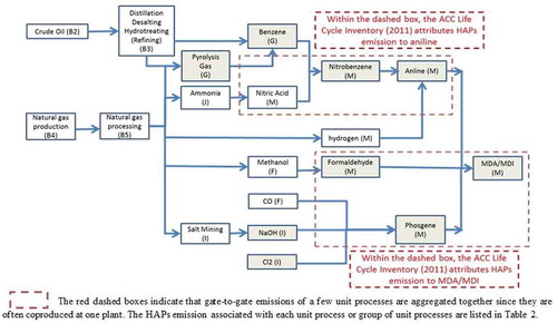
The system boundary defined for this case study is “cradle-to-gate,” which starts from raw material extraction and ends at the manufacturing plant where MDI is ready to be shipped (see Figure 1). The functional unit is 1000 kg of MDI produced. The unit processes to be included and studied in future site-specific modeling were identified by the following steps. First, on-site (i.e., gate-to-gate) emissions were obtained from the ACC report (American Chemistry Council 2011), as shown in Figure 1. It should be noted that the red dashed boxes indicate that gate-to-gate emissions of a few unit processes are aggregated together, since they are often co-produced at one plant. Second, unit processes that emit HAPs were identified based on the HAPs list (United States Congress 1990; EPA 2016), as shown in Table 2 under “site-specific dispersion modeling (exact location is known).” Third, the Directory of Chemical Producers (DCP) was used to locate the manufacturers of the identified unit process (e.g., benzene) (Stanford Research Institute 2011) for site-specific dispersion modeling. If the manufacturers could not be identified in the DCP, such as crude oil and natural gas, then the unit processes were excluded from site-specific modeling but included in the multimedia modeling. For cradle-to-gate MDI production, a total of five unit processes were identified for site-specific modeling and three unit processes were identified for multimedia modeling, as shown in Table 2. The remaining unit processes in this cradle-to-gate LCI do not have HAPs reported in the LCI developed by ACC.

Table 2. Classification of unit processes (based on ACC LCI; American Chemistry Council 2011) .

Model scenario	Unit process	HAPs emitted	Total no. of plants*
Site-specific dispersion modeling (Exact location is known)	Cl2 and NaOH	Benzene, CCl4, Cl2, Pb, and Hg(II)	14
	Aniline	Pb	5
	Pyrolysis gas (olefins)	Cl2	3
	Benzene	Cl2	16
	MDA/MDI	Cl2, formaldehyde, methanol, Cl2, and CCl4	4
Non-site-specific multimedia modeling (Exact location is unknown)	Crude oil production and processing	As(V), benzene, Cl2, Cr(VI), ethyl benzene, ethylene dibromide, Hg(II), Ni(II), PAH as B(a)P, Sb(V), toluene and xylene	N/A
	Natural gas production and processing
	Salt mining
Not modeled	Ammonia	No HAP emissions reported at the manufacturing site	N/A
	Methanol
	Hydrogen
	Carbon monoxide

*Total number of plants that were included for site-specific modeling that covers 85% of the annual production capacity.

Figure 1. The system boundary of cradle-to-gate MDI production (modified from American Chemistry Council 2011).

Developing a regionalized LCI (step 2)

In order to assess the inhalation risks of each unit process at the site-specific level, a regionalized LCI is required. The first step was geocoding the unit process identified in step 1. TRI is a publicly available database that contains the latitude and longitude coordinates of each plant (EPA 2018b). The geocoded plant locations were entered into a geographical information system (ArcGIS) (Environmental Systems Research Institute 2015). For certain unit processes (e.g., benzene) that have multiple plants (may be owned by the same company) in the United States, a cutoff criteria was applied as described below. All plants were ranked by their production capacities from the highest to the lowest, and the production capacities were summed. Only the plants (from the highest to the lowest production capacity) that contributed to the top 85% production capacity were included for site-specific modeling. For example, there were 36 plants in the United States that produce benzene, and the top 16 of them accounted for over 85% of the total production capacity (Stanford Research Institute 2011). Therefore, the cutoff criteria was set to include the top 16 plants (based on production capacity) in site-specific modeling. When two plants had the same capacity, the one in proximity to Houston, Texas, or Geismar, Louisiana, was selected, as these two locations are the primary regions of MDI production. Individual plant capacity was also recorded for future analysis.

Performing air dispersion modeling (step 3a)

EPA’s Human Exposure Model (HEM-3) with American Meteorological Society/U.S. Environmental Protection Agency Regulatory Model (AERMOD) (EPA 2018a) was used for site-specific air dispersion modeling. AERMOD is different from LCIA models, as it uses site-specific meteorological and geographical conditions to study the fate and transport of HAPs whereas LCIA approaches largely assume that the aforementioned conditions are homogenous within one environmental compartment. AERMOD calculates the concentration of airborne HAPs at a certain distance from the emission source. This concentration can be linked with a specific census block (i.e., receptor). The common trend is that the airborne concentration is higher at receptors that are closer to the emission sources. Key input files needed to perform such modeling include emission, meteorological, and surface terrain files.

In site-specific modeling, the amount of HAPs emitted from each unit process at an individual plant was calculated based on the functional unit (mt HAPs emitted per 1 mt MDI produced). All emissions were modeled as a point source located at the coordinates as previously geocoded in ArcGIS. One important component in the emission profile is the stack parameters. The NEI Standard Classification Code (SCC) average stack parameters were chosen for the unit processes, as listed in Table 3. Meteorological and surface terrain files were obtained from weather stations closest to the manufacturing plant according to the station list provided by HEM-3. A total of 36 unique plants that produced one or more of the five unit processes listed in Table 3 were modeled.

Table 3. Unit processes and site-specific modeling/average stack parameters (EPA 1999a) .

	Average stack parameters
Unit process	Height (m)	Diameter (m)	Exit velocity (m/sec)	Exit temperature (K)
Cl2 and NaOH	10.68	0.92	8.94	318.61
Aniline	16.73	1.17	8.20	399.73
Pyrolysis gas (olefins)	25.10	1.31	4.75	409.72
Benzene	14.67	0.23	0.31	297.13
MDA/MDI	5.87	0.12	1.00	315.28

Calculating inhalation risks of site-specific unit processes (step 3b)

Two human health end points (cancer and noncancer) were evaluated based on the modeled average airborne concentration of each HAP at a specific census block and its toxicity values in the reference library of HEM-3 (EPA 2017). At a specific census block, the cancer risk of HAPs by inhalation pathway was expressed mathematically as eq 1.

(1)

where C_i,j (μg/m³ per ton of HAP) is the modeled yearly average airborne concentration of HAP i at a specific census block based on 1 ton HAP i emission from plant j. URE_i (m³/μg) is the inhalation cancer unit risk estimate of HAP i, which represents the upper-bound excess lifetime cancer risk estimated to result from continuous exposure to a chemical at a concentration of 1 μg/m³ in air (EPA 1996). EF_i,k (emission factor, mt HAP i/mt MDI) is the amount of HAP i emitted from unit process k per functional unit (1000 kg MDI), PC_k,_j (%) is the plant j’s production capacity percentage among all plants that produce unit process k, P_MDI (mt) is the total MDI production capacity in the United States, m is the number of HAPs emitted from unit process k, n is the number of manufacturing plants that produce unit process k, and p is the number of unit processes identified for site-specific air dispersion modeling.

Similarly, noncancer risk of HAPs by inhalation pathway can be expressed as eq 2. The noncancer hazard index can be calculated as follows:

(2)

where RfC_i is the reference concentration for noncancer end points by inhalation pathway for HAP i. For chemicals with multiple noncancer end points, HEM-3 identifies all the targeted organs, but only the RfC that results in the highest HI is included in the toxicity value reference library.

An example calculation can be found in the supplementary information.

Calculating inhalation risks of non-site-specific unit processes (step 4)

For unit processes without exact production location as shown in Table 2, the USEtox model was used to perform screening level risk characterization. In this case study, the HAP emission rate (kg/day) of non-site-specific unit processes was calculated based on the emission factor per functional unit and then scaled by annual MDI production capacity. The HAPs were assumed to be released into the continental air compartment. For example, a total of 0.037 kg benzene is emitted from all non-site-specific unit processes per 1 metric ton of MDI produced. Based on the annual MDI production of 1.27 million metric tons in the United States, the average daily benzene emission is 129 kg. In the USEtox model, HAP emissions from non-site-specific unit processes created an emission rate matrix containing an entry for the continental air compartment only. The emission rate matrix was then multiplied by the fate factor matrix, which describes the fate and transport of HAPs amongst different environmental compartments. The product of these two matrices was the HAP mass in each compartment at steady state. Then the HAP mass was divided by the air compartment volume defined in USEtox to calculate the steady-state airborne concentration (urban: 5.76 × 10¹⁰ m³; continental: 1.00 × 10¹⁶ m³; global: 4.60 × 10¹⁷ m³). Following the Risk Assessment Guidance for Superfund (EPA 1989), the inhalation risk of each HAP was calculated using the steady-state airborne concentration and the toxicity values provided in the reference library of HEM-3. For the same benzene example, USEtox calculated the steady-state benzene concentration in continental air compartment at 4.18 × 10⁻⁵ μg/m³. The corresponding cancer risk was 3.26 × 10⁻¹⁰ and noncancer HI was 1.39 × 10⁻⁶. Finally, the inhalation risks associated with non-site-specific unit processes were calculated by adding the risk characterization values of all HAPs involved in USEtox modeling.

Combining the risk characterization values of all unit processes (step 5)

Finally, the total inhalation risks of the cradle-to-gate MDI production were calculated by adding the site-specific (step 3b) and non-site-specific (step 4) risk characterization values.

Identifying inhalation risk hot spots and patterns in GIS (step 6)

In HEM-3, the modeled airborne concentration is at the census block level, which is the smallest graphical unit in the census (United States Census Bureau 2015). However, due to model uncertainties, it has been shown in previous studies that census block– or census tract–level results should only be used to identify geographical patterns of human health risks instead of pinpointing any specific census block or tract (EPA 2015b). Therefore, this research investigated the census tract–level results to identify the geographical pattern of inhalation risks and used the total inhalation risk at the county level for risk characterization. The census block–level results were averaged within each census tract to represent tract-level results and plotted in ArcMap. Similarly, census tract results were averaged within each county to represent county-level results.

Results

As described in the method steps 4 and 5, inhalation risks associated with cradle-to-gate MDI production were calculated separately for the site-specific and non-site-specific unit processes.

Site-specific unit processes

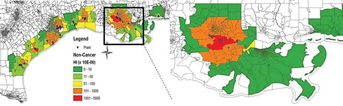
A total of 36 plants were included in the site-specific modeling, which covered the five unit processes listed in Table 3. All plants are located in the Gulf Coast region, including four states: Texas, Louisiana, Mississippi, and Alabama. Out of the 36 plants, 1 plant covers three unit processes, 4 plants cover two unit processes, and the remaining plants cover only one unit process each. The inhalation risks were first plotted at the census tract level in ArcGIS to illustrate the risk pattern in terms of plant locations (Figure 2). Then in Figure 3, the averaged census tract result was chosen to represent the entire county. The color scheme only shows the absolute values of inhalation risks and does not correspond to any risk management threshold values.

Figure 2. Census tract–level inhalation risks of site-specific unit processes (left: cancer risk; right: noncancer HI).

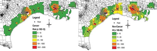
Figure 3. County-level average inhalation risks of site-specific unit processes (left: cancer risk; right: noncancer hazard index).

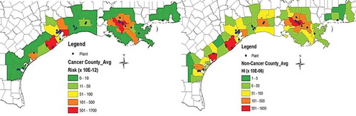
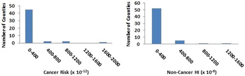
Overall, for the five unit processes involved in site-specific modeling, the accumulated inhalation risks ranged from 10⁻¹² to 10⁻⁹ for cancer risk and 10⁻⁶ to 10⁻³ for noncancer HI. At the county level, the highest average cancer risk was 1.70 × 10⁻⁹ at Ascension Parish, Louisiana, and the highest average noncancer HI was 1.53 × 10⁻³ at Iberville Parish, Louisiana. The majority of the county-level average inhalation risks were much lower than the highest values. As shown in Figure 4, the distribution of inhalation risk is skewed to the right for both cancer risk and noncancer HI, with the majority of counties at lower than 10⁻¹⁰ for cancer risk (45 out of 50) and 10⁻⁴ for noncancer HI (44 out of 59).

Figure 4. Distribution of inhalation risks associated with site-specific unit processes at the county level (left: cancer risk; right: noncancer hazard index).

In addition to the average inhalation risks shown at the county level, the census tract–level map reveals the spatial distribution of inhalation risks. Figures 5 and 6, demonstrate that higher potential inhalation risks occurred in regions that have manufacturing plants with greater production capacities. Two regions with relatively higher risks were identified: Houston and Baton Rouge. Production capacities in these regions can be found in Table 4. The four counties (Harris, Chamber, and Brazoria in Texas and Ascension Parish in Louisiana) in these two regions were among the highest cancer and noncancer risk counties out of a total of 59 counties evaluated. Plant production capacity was an important factor in determining the potential inhalation risks and their spatial distribution. The majority of aniline, olefins, and MDI were produced in these four counties, as shown in Table 4. In comparison, Jefferson County had four plants, which only supply 14.0% of aniline and 8.6% benzene and ranked the 20th for cancer risk and the 21st for noncancer HI out of the 59 counties evaluated.

Table 4. Production capacities of chemical plants in relatively high risk areas.

Area	No. of plants	Production capacities by mass
		Aniline	Benzene	Cl2/NaOH	Olefins	MDI
Houston	10	18.1%	37.1%	26.5%	48.2%	43.5%
Baton Rouge	7	55.3%	0%	6.0%	46.3%	56.5%
Sum	17	73.4%	37.1%	32.5%	94.5%	100%

Figure 5. Site-specific plant locations and high cancer risk areas.

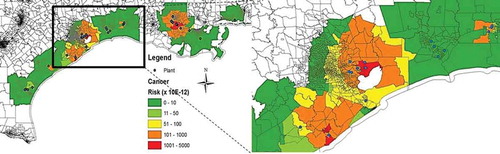
Figure 6. Site-specific plant locations and high noncancer hazard index areas.

All the plants modeled by site-specific modeling are located in the Gulf Coast, which is known to be the petrochemical corridor of the United States. However, the inhalation risks associated with MDI production varied among and within counties. The ratios between the highest risk and the lowest risk county were 14,457 for cancer risk and 1,369 for noncancer HI. Within the same county, inhalation risk pattern could have significant spatial variations. For example, the cancer risk of the highest census tract was about 20,000 times higher than the lowest one in Harris County, as shown in Figure S1. Such spatial differentiation revealed the limitation of existing LCIA models, which assume homogeneity within each environmental compartment. The site-specific modeling results showed that the variation in the same environmental compartment was not negligible. Therefore, the assumption that chemicals have a homogenous steady-state concentration in each environmental compartment may not be valid in cases where geographical variations are significant.

Non-site-specific unit processes

Site-specific modeling was not feasible for those unit processes with unknown production locations. Therefore, the USEtox model was used as an approach to assess inhalation risks associated with these unit processes, as explained in step 5 of the method. Table 5 shows the total inhalation risks of non-site-specific unit processes in each modeled environmental compartment. Urban and continental air compartments (cancer: 10⁻¹⁰; noncancer: 10⁻⁶) had similar risk results, which were 1 order of magnitude higher than the global air compartment (cancer: 10⁻¹¹; noncancer: 10⁻⁷). Figure 7 illustrates the relative contributions of HAPs to the inhalation risks. Benzene and nickel compounds were the two major contributors in all compartments, and ethylene dibromide accounted for about 21% of the total noncancer HI in the global air compartment. The relative contributions of HAPs were similar in urban and continental air compartments.

Table 5. Inhalation risks of unit processes without exact location (HAPs emitted to the continental air compartment).

Environmental compartment	Volume (m^3)	Cancer risk	Noncancer HI
Urban air	5.76 × 10^10	4.42 × 10^−10	4.46 × 10^−6
Continental air	1.00 × 10^16	4.61 × 10^−10	4.65 × 10^−6
Global air	4.60 × 10^17	2.13 × 10^−11	1.52 × 10^−7

Figure 7. Inhalation risks by HAPs for non-site-specific unit processes.

Total inhalation risks of cradle-to-gate MDI production

Risk characterization results of site-specific and non-site-specific unit processes were combined to derive the overall inhalation risks of cradle-to-gate MDI production. To be conservative, the highest risk of non-site-specific unit processes among air compartments (continental air) and the highest county-level risks of site-specific unit processes (Ascension Parish and Iberville Parish) were combined. The combined overall inhalation risks were 2.16 × 10⁻⁹ for cancer risk and 1.53 × 10⁻³ for noncancer HI. These levels are 3 orders of magnitude lower than the EPA risk management threshold values of 10⁻⁶ for cancer risk and 1 for noncancer HI (EPA 1999b).

Discussion

Comparisons between HEM-3/AERMOD and USEtox

In this study, two models were used to evaluate the unit processes in MDI production, depending on whether exact production location was known. Compared with the multimedia modeling (USEtox), the site-specific modeling (HEM-3/AERMOD) provides more information on the geographical distribution of inhalation risks. Table 6 shows that the inhalation risks of the cradle-to-gate MDI production can vary significantly in terms of geographical locations. The highest averaged county-level cancer risk at Ascension Parish, Louisiana, was 5 orders of magnitude higher than the lowest value at Wharton County, Texas. Similarly, for noncancer HI, this ratio was approximate 1400 between the highest value at Iberville Parish, Louisiana, and the lowest value at Stephens County, Texas.

Table 6. County-level inhalation risk statistics (AERMOD).

Risk level	Cancer Risk	Noncancer HI
Maximum	1.70 × 10^−9	1.54 × 10^−3
Median	1.84 × 10^−12	5.36 × 10^−5
Minimum	5.30 × 10^−14	1.12 × 10^−6

In order to demonstrate the differences between the two modeling approaches, a comparison was made by assuming all HAPs modeled in HEM-3/AERMOD (from site-specific processes) were emitted into the urban air compartment in USEtox. The mass of the HAPs that remained in the three air compartments (global, continental, and urban) at steady state was calculated and converted to concentration, using the volume of each environmental compartment. All the HAPs included in AERMOD were considered in USEtox except Cl₂, which has not been characterized in the most recent version of USEtox.

The results are shown in Table 7. For cancer risk, the urban, continental, and global air compartment results in USEtox were within 1 order of magnitude of the maximum, median, and minimum county-level results in HEM-3/AERMOD, respectively. However, for noncancer HI, only the urban air compartment result was within 1 order of magnitude of the maximum county-level result in HEM-3/AERMOD. One possible reason of USEtox underestimating the noncancer HI is the lack of characterization factor of Cl₂. Such results also show that inhalation risks can vary significantly within the modeled domain (50 km radius from the source), when HAPs were evaluated using HEM-3/AERMOD. In fact, the USEtox model can only calculate one risk value per air compartment based on the steady-state concentration. Without accounting for the geographical differences, assuming a homogenous environmental compartment could potentially over- or underestimate inhalation risks. Therefore, HEM-3/AERMOD can better characterize the inhalation risk of emissions if the production location is available, since in a real-world scenario, many factors may cause the homogeneous condition assumed in USEtox to be invalid. These factors are the relative location of the receptor to emission source, meteorological and terrain conditions in a specific region/site, and removal mechanisms of chemicals such as dry and wet depositions. Due to the nonhomogeneous nature of each environmental compartment, the lack of geographical granularity limits the use of USEtox beyond a high-throughput tool in human health assessment.

Table 7. Inhalation risks of site-specific unit processes (if using USEtox) (assuming that HAPs were emitted to the urban air compartment).

Environmental compartment	Cancer risk	Noncancer HI
Urban air	1.99 × 10^−9	5.42 × 10^−4
Continental air	1.14 × 10^−12	8.98 × 10^−8
Global air	3.25 × 10^−13	1.64 × 10^−9

Impact of emission compartments in USEtox

This research demonstrates the possibility of tracking exact emission locations of unit processes using publicly available data. However, such data are not always available for all unit processes. In this case study, natural gas, crude oil, and salt production were not included in the Directory of Chemical Producers. The selection of the emission compartment in USEtox could impact risk characterization of the non-site-specific unit processes. If the HAPs of the aforementioned three unit processes were emitted to the urban air compartment (Table 8) instead of the continental air compartment (Table 5), inhalation risks in urban air compartment would increase by 4 orders of magnitude for both cancer risk and noncancer HI. The cancer risk in the urban air compartment alone was even higher than the 10⁻⁶ risk management threshold value. Such difference in risk characterization demonstrates the need of regionalized LCI and the importance of identifying the HAP emission locations.

Table 8. Inhalation risks of non-site-specific unit processes (assuming that HAPs were emitted to the urban air compartment).

Environmental compartment	Cancer risk	Noncancer HI
Urban air	1.83 × 10^−6	2.32 × 10^−2
Continental air	4.60 × 10^−10	4.62 × 10^−6
Global air	2.13 × 10^−11	1.52 × 10^−7

Relative unit process contribution to the inhalation risks

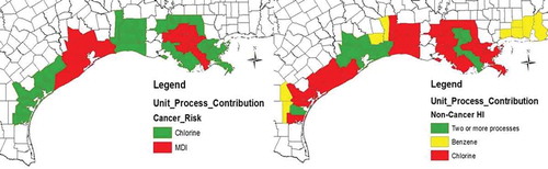
In the interpretation step of an LCA, the indicator results are often presented by unit process, so that high-impact processes can be identified. However, since the human health LCIA is conducted at continental or global scale, such analysis fails to reveal the relative contribution of each unit process at different geographical locations. In this research, site-specific modeling results were analyzed to determine which unit processes contribute the most to the averaged county-level inhalation risks (Figure 8). In this cradle-to-gate LCI, among the five unit processes modeled using AERMOD, only two unit processes (MDI and Cl₂) emitted HAPs that have carcinogenic effect. All five unit processes contributed to the noncancer HI. HAPs emitted from Cl₂ production contributed 100% to the cancer risk in 31 out of the 50 counties, and HAPs emitted from MDI production (gate-to-gate) contributed more than Cl₂ production in the remaining 19 counties. In terms of noncancer HI, 14 out of 59 counties had at least two unit processes that contributed more than 10% of the overall inhalation risk. Most of the counties are located in the two relatively high inhalation risk regions (Houston and Baton Rouge). In other regions, Cl₂ production had the highest impact; it alone contributed more than 70% of the noncancer HI in 36 counties. In this analysis, HEM-3/AERMOD enabled us to identify the top contributing unit processes in different regions. The results can guide decision makers to reduce the human health impact of MDI supply chain, with a focus on specific unit process in a high-risk region. For example, in the two counties with highest cancer risk (Ascension Parish, Louisiana) and noncancer HI (Iberville Parish, Louisiana), HAP reduction should focus on the unit processes of Cl₂ and MDI, since they were the highest contributing unit processes.

Figure 8. Relative contributions of unit processes to inhalation risks.

Limitation of this study

The ACC MDI LCI only includes HAPs based on the EPA’s HAP list. However, there could be other air pollutants that may cause adverse health outcomes that were not included. The reporting responsibilities of those air pollutants outside the EPA’s HAP list vary by states. Future work should be expanded to include those air pollutants that are in the state emission inventory but not the federal EPA’s HAP list.

USEtox results indicate that inhalation may not be the primary exposure pathway of certain chemicals. The steady-state mass distribution of HAPs among different environmental compartments depends on chemical characteristics such as vapor pressure, octanol-water partition coefficient, and degradation constant. Among the 11 HAPs modeled in USEtox, only 5 had the majority of mass partitioned in the air compartments at the steady-state condition. Table 9 shows the mass distribution of HAPs when they were emitted to the continental air compartment. Although Nickel(II) contributed significantly to the total inhalation risks (Figure 7), only a tiny amount of nickel stayed in the air compartment. Similar results can be found for other inorganics, of which very little mass stayed in the air compartment at steady state while most of the mass was distributed into the soil compartment. Therefore, ingestion pathway should be included in future studies to evaluate the overall health risks of these inorganics in addition to the inhalation pathway.

Table 9. Mass distributions of HAPs in different environmental compartments.

HAP	Air compartment (%)	Water compartment(%)	Soil compartment (%)
As(V)	4.81 × 10^−3	6.57	93.4
Benzene	89.2	10.7	5.59 × 10^−3
Cr(VI)	4.41 × 10^−2	33.8	66.2
Ethyl benzene	98.0	1.88	0.152
Ethylene dibromide	72.1	27.5	0.484
Hg(II)	7.23 × 10^−4	7.39 ×10^−2	99.9
Ni(II)	6.53 × 10^−5	33.4	66.6
PAH as B(a)P	1.03	11.5	87.4
Sb(V)	2.30 × 10^−2	46.9	53.1
Toluene	97.4	2.47	0.127
Xylene	97.6	2.12	0.256

Notes. HAPs with the majority of the mass distributed in the air compartment at steady state are in bold.

This research evaluated the inhalation risks associated with cradle-to-gate MDI production but did not include downstream use of MDI. Future work should apply indoor fate and transport models to evaluate the health risks of downstream products that are made from MDI such as foam insulation.

Conclusion

Air dispersion modeling and LCA together can provide a holistic view of the human health risks of a chemical. Many current human health LCIA models assume that environmental compartments are homogeneous and perform assessment under steady-state conditions. However, such assumption lacks the ability to identify the geographical differences and patterns of human health risks, which is an essential piece of information for decision makers to mitigate risk and improve manufacturing processes. A current challenge is to increase the geographical relevance of HHIA without using confidential business information or proprietary data. This research demonstrates the development of a regionalized LCI using publicly available data and illustrates the application of site-specific air dispersion modeling together with USEtox to assess the inhalation risk of chemicals along the supply chain. To the best of our knowledge, this work derives the first regionalized LCI of a chemical for the industry using publicly available data and evaluates inhalation risks along its cradle-to-gate production. With regionalized LCI, air dispersion modeling can be performed simultaneously for multiple facilities and unit processes in multifacility HEM-3. The case study used MDI as an example, but this method can be applied to any other chemicals or products to address the question often faced by decision makers: “Is manufacturing certain products along the life cycle adding unacceptable risk to the society?”

The case study results showed that the conservative overall inhalation risks of cradle-to-gate MDI were 3 orders of magnitude lower than the EPA risk management threshold values. In addition, it was found that the highest inhalation risks occurred in two counties in Louisiana where HAPs emitted from Cl₂ and MDI production (gate-to-gate) contributed the most risks. The advantage of employing site-specific air dispersion modeling is that geographical relevance in human health LCIA is increased by better understanding the spatial pattern of risks. As a result, pollution reduction and risk management actions can be implemented more efficiently.

This work illustrates that whenever feasible, site-specific air dispersion modeling should be considered. For many chemicals used as raw materials in commerce, the production location and capacity can be obtained using publicly available data. However, such data for some other chemicals (e.g., crude oil and salt) are not always available. To improve the geographical relevance, emission inventory, manufacturer location, and production capacity data should be continually collected and made publicly available.

In future studies, additional exposure pathways need to be evaluated for release of inorganic HAPs to the air. It will require regionalized or site-specific information on watersheds and agricultural production. Furthermore, downstream applications and disposal options should be included to assess the overall health risks along the rest of life cycle phases. In general, human health assessment could benefit by embracing life cycle thinking and employing the site-specific modeling to increase geographical relevance.

supplemental data

Supplemental data for this paper can be access on the publisher’s website..

Additional information

Funding

Shen Tian also works at Covestro LLC, and Covestro funds his research at the University of Pittsburgh through tuition support.

Notes on contributors

Shen Tian

Shen Tian is a senior environmental engineer at Covestro LLC and a Ph.D. candidate at the Civil and Environmental Engineering Department, University of Pittsburgh.

Melissa Bilec

Melissa Bilec is an Associate Professor with the Civil and Environmental Engineering Department at the University of Pittsburgh and the Deputy Director at the Mascaro Center for Sustainable Innovation.

References

- Afshar, A. A. 2014. Chemical profile: Methylene diphenyl diisocyanate. Accessed March 23, 2018. http://www.chemplan.biz/(X(1)S(r05csalpuogmwlo1c3mrhj4g))/chemplan_demo/sample_reports/MDI_Profile13.pdf.
- American Chemistry Council. 2011. Cradle-to-gate life cycle inventory of nine plastic resins and four polyurethane precursors. Washington, DC: American Chemistry Council.
- American Chemistry Council. 2015. What are diisocyanates? Accessed March 21, 2018. http://dii.americanchemistry.com/Diisocyanates-Explained/What-Are-Diisocyanates.
- American Chemistry Council. 2016. American chemistry: The cornerstone of our economy. Accessed March 21, 2018. https://www.americanchemistry.com/Jobs/EconomicStatistics/American-Chemistry-The-Cornerstone-of-our-Economy.pdf.
- Bare, J. 2011. TRACI 2.0: The tool for the reduction and assessment of chemical and other environmental impacts 2.0. Clean Technol. Environ. Policy 13 (5):687–696. doi:10.1007/s10098-010-0338-9.
- Biryol, D., C. I. Nicolas, J. Wambaugh, K. Phillips, and K. Isaacs. 2017. High-throughput dietary exposure predictions for chemical migrants from food contact substances for use in chemical prioritization. Environ. Int. 108:185–194. doi:10.1016/j.envint.2017.08.004.
- Bonnell, M. A., A. Zidek, A. Griffiths, and D. Gutzman. 2018. Fate and exposure modeling in regulatory chemical evaluation: New directions from retrospection. Environ. Sci.: Process. Impacts 20 (1):20–31. doi:10.1039/C7EM00510E.
- Bureau of Economic Analysis. 2016. Gross-Domestic-Product-(GDP)-by-industry data. Accessed March 21, 2018. http://www.bea.gov/industry/gdpbyind_data.htm.
- Centers for Disease Control and Prevention. 2012. The different types of health assessments. Accessed March 21, 2018. https://www.cdc.gov/healthyplaces/types_health_assessments.htm.
- Environmental Systems Research Institute. 2015. ArcGIS desktop 10.2.. Redlands, CA.
- Harder, R., H. Holmquist, S. Molander, M. Svanstrom, and G. M. Peters. 2015. Review of environmental assessment case studies blending elements of risk assessment and life cycle assessment. Environ. Sci. Technol. 49 (22):13083–13093. doi:10.1021/acs.est.5b03302.
- Hellweg, S., E. Demou, R. Bruzzi, A. Meijer, R. K. Rosenbaum, M. A. J. Huijbregts, and T. E. McKone. 2009. Integrating human indoor air pollutant exposure within life cycle impact assessment. Environ. Sci. Technol. 43 (6):1670–1679. doi:10.1021/es8018176.
- Humbert, S., R. Manneh, S. Shaked, C. Wannaz, A. Horvath, L. Deschenes, O. Jolliet, and M. Margni. 2009. Assessing regional intake fractions in North America. Sci. Total Environ. 407 (17):4812–4820. doi:10.1016/j.scitotenv.2009.05.024.
- Isaacs, K. K., W. G. Glen, P. Egeghy, M. R. Goldsmith, L. Smith, D. Vallero, R. Brooks, C. M. Grulke, and H. Ozkaynak. 2014. SHEDS-HT: An integrated probabilistic exposure model for prioritizing exposures to chemicals with near-field and dietary sources. Environ. Sci. Technol. 48 (21):12750–12759. doi:10.1021/es502513w.
- Morello‐Frosch, R., A. T. J. Woodruff, D. A. Axelrad, and J. C. Caldwell. 2000. Air toxics and health risks in California: The public health implications of outdoor concentrations. Risk Anal. 20 (2):273–292. doi:10.1111/0272-4332.202026.
- Moriguchi, Y., and A. Terazono. 2000. A simplified model for spatially differentiated impact assessment of air emissions. Int J. Life Cycle Assess. 5 (5):281. doi:10.1007/bf02977580.
- Neumann, C. M., D. L. Forman, and J. E. Rothlein. 1998. Hazard screening of chemical releases and environmental equity analysis of populations proximate to toxic release inventory facilities in Oregon. Environ. Health Perspect. 106 (4):217–226.
- Olsen, S. I., F. M. Christensen, M. Hauschild, F. Pedersen, H. F. Larsen, and J. Tørsløv. 2001. Life cycle impact assessment and risk assessment of chemicals — A methodological comparison. Environ. Impact Assess. Rev. 21 (4):385–404. doi:10.1016/S0195-9255(01)00075-0.
- Potting, J., M. Hauschild, and H. Wenzel. 1999. “Less is better” and “only above threshold”: Two incompatible paradigms for human toxicity in life cycle assessment? Int. J. Life Cycle Assess. 4 (1):16–24. doi:10.1007/bf02979391.
- Rosenbaum, R. K., A. Meijer, E. Demou, S. Hellweg, O. Jolliet, N. L. Lam, M. Margni, and T. E. McKone. 2015. Indoor air pollutant exposure for life cycle assessment: Regional health impact factors for households. Environ. Sci. Technol. 49 (21):12823–12831. doi:10.1021/acs.est.5b00890.
- Rosenbaum, R. K., M. J. Huijbregts, A. Henderson, M. Margni, T. McKone, D. Meent, M. Hauschild, S. Shaked, D. Li, L. Gold, and O. Jolliet. 2011. USEtox human exposure and toxicity factors for comparative assessment of toxic emissions in life cycle analysis: Sensitivity to key chemical properties. Int. J. Life Cycle Assess. 16 (8):710–727. doi:10.1007/s11367-011-0316-4.
- Rosenbaum, R. K., T. Bachmann, L. Gold, M. J. Huijbregts, O. Jolliet, R. Juraske, A. Koehler, H. Larsen, M. MacLeod, M. Margni, T. McKone, J. Payet, M. Schuhmacher, D. Meent, and M. Hauschild. 2008. USEtox—The UNEP-SETAC toxicity model: Recommended characterisation factors for human toxicity and freshwater ecotoxicity in life cycle impact assessment. Int. J. Life Cycle Assess. 13 (7):532–546. doi:10.1007/s11367-008-0038-4.
- Sleeswijk, A. 2011. Regional LCA in a global perspective. A basis for spatially differentiated environmental life cycle assessment. Int. J. Life Cycle Assess. 16 (2):106–112. doi:10.1007/s11367-010-0247-5.
- Sonnemann, G., F. Castells, and M. Schuhmacher. 2004. Integrated life-cycle and risk assessment for industrial processes. USA: Lewis Publishers.
- Spadaro, J. V., and A. Rabl. 1999. Estimates of real damage from air pollution: Site dependence and simple impact indices for LCA. Int. J. Life Cycle Assess. 4 (4):229. doi:10.1007/bf02979503.
- Stanford Research Institute. 2011. Directory of chemical producers: United States of America. Menlo Park, CA: Chemical Information Services, Stanford Research Institute.
- Tam, B. N., and C. M. Neumann. 2004. A human health assessment of hazardous air pollutants in Portland, OR. J. Environ. Manage. 73 (2):131–145. doi:10.1016/j.jenvman.2004.06.012.
- Thinkstep. 2014. GaBi LCA databases. Accessed March 21, 2018. http://www.gabi-software.com/databases/gabi-databases/.
- U.S. Environmental Protection Agency. 1989. Risk assessment guidance for superfund. In Human health evaluation manual (Part A). , ed.. Vol. I. Washington, D.C: U.S. Environmental Protection Agency. .
- U.S. Environmental Protection Agency. 1996. Technology transfer network: 1996 national-scale air toxics assessment - Unit Risk Estimate (URE). Accessed March 21, 2018. https://archive.epa.gov/airtoxics/nata/web/html/gloadd.html.
- U.S. Environmental Protection Agency. 1999a. Estimate of stack heights and exit gas velocities for TRI facilities in OPPT’s risk-screening environmental indicators model, June 1999. Accessed May 5, 2018. https://www.epa.gov/rsei/estimate-stack-heights-and-exit-gas-velocities-tri-facilities-oppts-risk-screening.
- U.S. Environmental Protection Agency. 1999b. Residual risk - report to congress. In Office of air quality planning and standards, ed. 27711. Research Triangle Park, NC: U.S. Environmental Protection Agency.
- U.S. Environmental Protection Agency. 2015a. Assessing and managing chemicals under TSCA: Methylene Diphenyl Diisocyanate (MDI) and related compounds. Accessed March 21, 2018. https://www.epa.gov/assessing-and-managing-chemicals-under-tsca/methylene-diphenyl-diisocyanate-mdi-and-related.
- U.S. Environmental Protection Agency. 2015b. Technical support document EPA’s 2011. National-scale Air Toxic Assessment. Research Triangle Park, NC: U.S. Environmental Protection Agency.
- U.S. Environmental Protection Agency. 2016. Modifications to the 112(b)1 hazardous air pollutants. Accessed March 21, 2018. https://www3.epa.gov/airtoxics/pollutants/atwsmod.html.
- U.S. Environmental Protection Agency. 2017. Download Human Exposure Model (HEM). Accessed December 10, 2017. https://www.epa.gov/fera/download-human-exposure-model-hem.
- U.S. Environmental Protection Agency. 2018a. Human exposure modeling - overview. Accessed March 21, 2018. https://www.epa.gov/fera/human-exposure-modeling-overview.
- U.S. Environmental Protection Agency. 2018b. Toxics Release Inventory (TRI) program. Accessed March 21, 2018. https://www.epa.gov/toxics-release-inventory-tri-program.
- U.S. Environmental Protection Agency. 2005. Human health risk assessment protocol. In Office of solid waste and emergency response, ed. Washington, D.C: U.S. Environmental Protection Agency.
- United States Census Bureau. 2015. Census blocks. Accessed March 21, 2018. https://www.census.gov/geo/reference/webatlas/blocks.html.
- United States Congress. 1990. 42 U.S.C. chapter 85-air pollution prevention and control, section 7412. Washington, D.C.: U.S. Government Printing Office.
- United States Congress. 2016. H.R.2576 - Frank R. Lautenberg chemical safety for the 21st century act, ed. Washington, D.C: House - Energy and Commerce.
- United States Government Accountability Office. 2013. Chemical regulation: Observations on the toxic substances control act and EPA implementation. In United states government accountability office, ed.. 20548. Washington, DC: U.S. Governmental Accountability Office.
- Walser, T., R. Juraske, E. Demou, and S. Hellweg. 2014. Indoor exposure to toluene from printed matter matters: Complementary views from life cycle assessment and risk assessment. Environ. Sci. Technol. 48 (1):689–697. doi:10.1021/es403804z.
- Wambaugh, J. F., A. Wang, K. L. Dionisio, A. Frame, P. Egeghy, R. Judson, and R. W. Setzer. 2014. High throughput heuristics for prioritizing human exposure to environmental chemicals. Environ. Sci. Technol. 48 (21):12760–12767. doi:10.1021/es503583j.
- Wambaugh, J. F., R. W. Setzer, D. M. Reif, S. Gangwal, J. Mitchell-Blackwood, J. A. Arnot, O. Joliet, A. Frame, J. Rabinowitz, T. B. Knudsen, R. S. Judson, P. Egeghy, D. Vallero, and E. A. Cohen Hubal. 2013. High-throughput models for exposure-based chemical prioritization in the expocast project. Environ. Sci. Technol. 47 (15):8479–8488. doi:10.1021/es400482g.
- Wegener Sleeswijk, A., and R. Heijungs. 2010. GLOBOX: A spatially differentiated global fate, intake and effect model for toxicity assessment in LCA. Sci. Total Environ. 408 (14):2817–2832. doi:10.1016/j.scitotenv.2010.02.044.
- Weidema, B., C. Bauer, R. Hischier, and C. Mutel. 2013. The ecoinvent database: Overview and methodology, Data quality guideline for the ecoinvent database version 3. Accessed March 21, 2018. https://www.ecoinvent.org/files/dataqualityguideline_ecoinvent_3_20130506.pdf.
- Yurika, N., J. I. Levy, G. A. Norris, W. Andrew, H. Patrick, and J. D. Spengler. 2002. Integrating Risk assessment and life cycle assessment: A case study of insulation. Risk Anal. 22 (5):1003–1017. doi:10.1111/1539-6924.00266.
- Zelm, R., M. J. Huijbregts, and D. Meent. 2009. USES-LCA 2.0—A global nested multi-media fate, exposure, and effects model. Int. J. Life Cycle Assess. 14 (3):282–284. doi:10.1007/s11367-009-0066-8.