Advances in science and applications of air pollution monitoring: A case study on oil sands monitoring targeting ecosystem protection

ABSTRACT

The potential environmental impact of air pollutants emitted from the oil sands industry in Alberta, Canada, has received considerable attention. The mining and processing of bitumen to produce synthetic crude oil, and the waste products associated with this activity, lead to significant emissions of gaseous and particle air pollutants. Deposition of pollutants occurs locally (i.e., near the sources) and also potentially at distances downwind, depending upon each pollutant’s chemical and physical properties and meteorological conditions. The Joint Oil Sands Monitoring Program (JOSM) was initiated in 2012 by the Government of Canada and the Province of Alberta to enhance or improve monitoring of pollutants and their potential impacts. In support of JOSM, Environment and Climate Change Canada (ECCC) undertook a significant research effort via three components: the Air, Water, and Wildlife components, which were implemented to better estimate baseline conditions related to levels of pollutants in the air and water, amounts of deposition, and exposures experienced by the biota. The criteria air contaminants (e.g., nitrogen oxides [NO_x], sulfur dioxide [SO₂], volatile organic compounds [VOCs], particulate matter with an aerodynamic diameter <2.5 μm [PM_2.5]) and their secondary atmospheric products were of interest, as well as toxic compounds, particularly polycyclic aromatic compounds (PACs), trace metals, and mercury (Hg). This critical review discusses the challenges of assessing ecosystem impacts and summarizes the major results of these efforts through approximately 2018. Focus is on the emissions to the air and the findings from the Air Component of the ECCC research and linkages to observations of contaminant levels in the surface waters in the region, in aquatic species, as well as in terrestrial and avian species. The existing evidence of impact on these species is briefly discussed, as is the potential for some of them to serve as sentinel species for the ongoing monitoring needed to better understand potential effects, their potential causes, and to detect future changes. Quantification of the atmospheric emissions of multiple pollutants needs to be improved, as does an understanding of the processes influencing fugitive emissions and local and regional deposition patterns. The influence of multiple stressors on biota exposure and response, from natural bitumen and forest fires to climate change, complicates the current ability to attribute effects to air emissions from the industry. However, there is growing evidence of the impact of current levels of PACs on some species, pointing to the need to improve the ability to predict PAC exposures and the key emission source involved. Although this critical review attempts to integrate some of the findings across the components, in terms of ECCC activities, increased coordination or integration of air, water, and wildlife research would enhance deeper scientific understanding. Improved understanding is needed in order to guide the development of long-term monitoring strategies that could most efficiently inform a future adaptive management approach to oil sands environmental monitoring and prevention of impacts.

Implications: Quantification of atmospheric emissions for multiple pollutants needs to be improved, and reporting mechanisms and standards could be adapted to facilitate such improvements, including periodic validation, particularly where uncertainties are the largest. Understanding of baseline conditions in the air, water and biota has improved significantly; ongoing enhanced monitoring, building on this progress, will help improve ecosystem protection measures in the oil sands region. Sentinel species have been identified that could be used to identify and characterize potential impacts of wildlife exposure, both locally and regionally. Polycyclic aromatic compounds are identified as having an impact on aquatic and terrestrial wildlife at current concentration levels although the significance of these impacts and attribution to emissions from oil sands development requires further assessment. Given the improvement in high resolution air quality prediction models, these should be a valuable tool to future environmental assessments and cumulative environment impact assessments.

Introduction

The Canadian Oil Sands (OS) are predominantly located in the northern half of Alberta, with a small portion in central-western Saskatchewan. In size, the OS is 142,000 km² and is estimated to include approximately 1.7 trillion barrels of oil in the form of bitumen, although the recoverable amount of oil is only about 10% of that amount, or 163.4 billion barrels (Natural Resources Canada, Canada 2017). This still makes the OS the third largest known reserve of oil on earth. Once recovered, bitumen, which is highly viscous and enriched in sulfur, carbon, nitrogen, and metals and deficient in hydrogen compared with conventional and heavy crude oil, requires upgrading. The bitumen extraction, separation, and upgrading processes that ultimately produce synthetic crude oil consume energy and resources and produce waste, which can pose environmental risks.

J.R. Brook

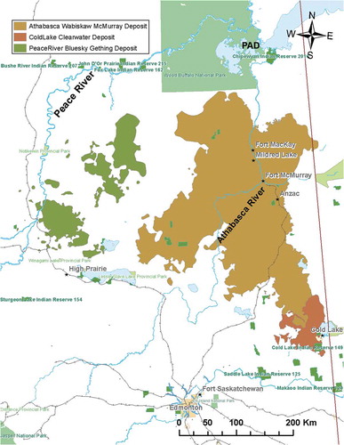
Two major rivers, the Peace River and the Athabasca River (AR), both originating from headwaters in the Rocky Mountains, flow through the OS region. The glacial-fed Athabasca River is the longest in Alberta; its watershed encompasses nearly one quarter of the province. From its mountainous origins, it flows for approximately 1000 km before encountering the large, near-surface deposits of bitumen in the area just north of Fort McMurray, the largest city in the region (population of the Regional Municipality of Wood Buffalo, which includes the city, was 71,589 in 2016). The Athabasca River is a source of drinking water for Fort McMurray, and the river is an essential source of fresh water for bitumen recovery and processing. Both rivers empty into Lake Athabasca; to the west of Lake Athabasca they form the Peace-Athabasca Delta (PAD), which is also 200 km downstream from where the Athabasca River flows through the near-surface OS deposits. The PAD is one of the largest freshwater deltas on earth and has been designated as a wetland of international importance (through the Ramsar Convention) and a United Nations Educational, Scientific and Cultural Organization (UNESCO) World Heritage Site. The PAD is also partially within Wood Buffalo National Park. Figure 1 includes a map that provides perspective for the area.

Figure 1. Northern Alberta showing the Athabasca River, the Peace River, the Peace-Athabasca Delta (PAD), and the oil sands deposits.

There is tremendous biodiversity in the PAD, with millions of migratory birds passing through annually. The Lower Athabasca River (LAR) subbasin contains Fort McMurray, the majority of the OS deposits, the McMurray Formation, and the PAD. Indigenous inhabitants of the region include the Mikisew Cree First Nation and Athabasca Chipewyan First Nation, with traditional lands in the region downstream of Fort McMurray, including the PAD. Others include the Fort McKay First Nation, the Fort McMurray First Nation, and Métis Locals who have traditional lands near Fort McMurray and in and around the active oil sands surface mining region. Oil sands development poses potential risks to the environmental health of this part of Canada as well as to the populations residing there. Consequently, effective environmental management of the OS development is an essential responsibility of all stakeholders.

The potential value of the OS has been recognized for over a century, but economically viable processes to recover this “unconventional” oil from deposits near the surface became available in the second half of the 1960s. Advances in technology for extraction and in environmental protection have been continual since that time, including approaches to access what constitutes the majority (approximately 80%) of the bitumen that is farther below the surface using in situ techniques (because OS deposits that start deeper than about 70 m are not accessible through open-pit mining, in situ extraction approaches are required). Collectively, through these two processes, production in the OS has been yielding on the order of 2.7 million barrels of oil per day (Natural Resources Canada, Canada 2017) from 0.45 million cubic meters (m³) of raw bitumen processed per day (Alberta Energy Regulator, Canada 2017).

An important driver for technical advance in the OS industry has been to increase the ratio of bitumen production to energy input, which represents both an economic and an environmental benefit. Water consumption has been another key driver, with the main options for enhanced environmental performance being reduction in the amount of freshwater required for bitumen recovery and processing; water recycling, which leads to innovation in the clearing in fine suspended tailings in the ponds; and use of more deep, saline groundwater in the in situ process. Cleanup of tailings pond water, for reuse and eventual release into the watershed so that the land can be reclaimed, is another key challenge. With these and other accomplishments, the current OS industry represents an impressive engineering achievement for this important economic driver of the Canadian economy.

Motivation for the Joint Oil Sands Monitoring Program (JOSM)

The environmental performance of OS development has been under considerable public scrutiny. The prevailing narrative continually positions their significant contribution to Canada’s economy and energy security against potential environmental damage and impact to First Nations communities (Dowdeswell et al. 2010). Understanding the extent of the potential environmental damage so that its characteristics, magnitude, and long-term implications can inform public debate and public policy decisions about development is critical. However, there has been debate concerning the availability of open, transparent, and credible data sources that could be used in making sound, evidence-based policy and regulatory decisions in the OS region. The scale and scope of the OS development means that environmental impact is likely, and some level of management of this impact is required.

Given the importance to Canada, a Royal Society of Canada (RSC) panel was tasked with undertaking a comprehensive, evidence-based assessment of the major environmental and health impacts of Canada’s OS industry. The RSC panel sought to offer Canadians an independent review assessing the available evidence and identifying knowledge gaps (The Royal Society of Canada 2010; Weinhold 2011). The Canadian Federal Minister of the Environment also established a panel (OS Advisory panel), charged with “Documenting, reviewing and assessing the current body of scientific research and monitoring” and “Identifying strengths and weaknesses in the scientific monitoring, and the reasons for them” (Dowdeswell et al. 2010). The findings of these two panels, released in 2010, provide context for the initiation of JOSM (Joint Canada-Alberta Implementation Plan for Oil Sands Monitoring 2012). Their full reports are available (Dowdeswell et al. 2010; The Royal Society of Canada 2010), and an overview of their findings in the context of this critical review is provided in Section S1.1 of the supplemental material.

The OS Advisory panel’s overarching recommendation was that a shared national vision and management framework of aligned priorities, policies, and programs be developed collaboratively by relevant jurisdictions and stakeholders based upon four key fundamentals: “An holistic and integrated approach, An adaptive approach, A credible scientific approach, and A transparent and accessible approach.” The RSC panel’s view was that the lack of availability of environmental data collected by current developments and operations in the OS region meant that timely, comprehensive assessments of the data were not taking place and that, consistent with the OS Advisory panel’s findings, providing wider access to monitoring data was a priority for improving cumulative impact assessment. JOSM was established, at least partially, in response to this priority.

The scope of this critical review

This critical review covers the main objectives and findings of the (now) Environment and Climate Change Canada (ECCC) research and monitoring supporting JOSM, with an emphasis on atmospheric emissions and their potential impacts on air quality and deposition and linkages to water quality and potential impacts on wildlife. The conclusions and gaps summarized from this ECCC work are generally reflective of reports and publications up through approximately 2018. In addition to ECCC scientific results, some of the existing knowledge and activities prior to the enhanced efforts brought about by the implementation of JOSM, and some of the non-JOSM work, are discussed in this critical review. Landscape disruption and habitat loss have long-term influences on wildlife and ecosystems, and attention is being paid to this issue in the OS (Alberta Biodiversity Monitoring Institute, Canada 2019), but are not discussed in this review. Greenhouse gas emissions are also a critical issue for the OS but are outside the scope of this review. Human health effects are also a potential concern and were discussed by the RSC panel, but they are also not covered in this review.

JOSM is a partnership involving both the Province of Alberta and the Government of Canada. Given that the focus of this review is largely on scientific work undertaken at ECCC in the context of air emissions, it does not represent a full review of the JOSM science or program. Nonetheless, recognizing that it is helpful to take stock of scientific progress on a regular basis to guide future work, it is hoped that this critical review can play a role in ECCC’s integrated planning and may also contribute to a future full JOSM science integration and assessment (i.e., federal and provincial findings), ultimately supporting adaptive management of OS ecosystem impact monitoring.

This critical review consists of (1) objectives of JOSM and evidence of impacts; (2) challenges of assessing ecosystem effects; (3) main findings from the Air Component; Air Component applications to the (4) Water and (5) Wildlife Contaminants and Toxicology Component; and (6) concluding remarks. Two “integrating themes” were of interest across components: polycyclic aromatic compounds (PACs) and mercury. A summary on PAC integration (Harner et al. 2018) is reported in this critical review. The issue of acid deposition was considered in an integrated manner, building upon a long monitoring history in this area (i.e., the Acid Rain Program beginning in the 1970s), and results are highlighted in this critical review (Makar et al. 2018).

JOSM objectives

Expanding upon the recommendations of the EC Panel, JOSM’s main objectives (Joint Canada-Alberta Implementation Plan for Oil Sands Monitoring 2012) were

1. Support sound decision‐making by governments as well as stakeholders

2. Ensure transparency through accessible, comparable, and quality‐assured data

3. Enhance science‐based monitoring for improved characterization of the state of the environment and collect the information necessary to understand cumulative effects

4. Improve analysis of existing monitoring data to develop a better understanding of historical baselines and changes

5. Reflect the transboundary nature of the issue and promote collaboration with the governments of Saskatchewan and the Northwest Territories

At the beginning of JOSM implementation there was extensive existing monitoring in the OS region (Figure S1.1), and the starting goals for JOSM were to enhance/improve these activities. In practice, multiple focused monitoring or research projects, mainly pertinent to objectives 3 and 4, were initiated by ECCC to characterize general baseline conditions and develop methods useful to detect changes in the environment in order to make progress on understanding cumulative effects.

Evidence of potential impacts

There were at least five lines of evidence that informed JOSM studies:

• Snowpack measurements

• Historical cores of lake sediments and peat

• Air monitoring

• Samples of the biota (e.g., lichen or wildlife)

• Atmospheric modeling results

Kelly et al. (Kelly et al. 2010, 2009) measured PACs and metals in snow at multiple locations in the OS development area. There was a clear decrease in the amount deposited in the snowpack in relation to distance from the OS operations. The work also demonstrated that pollutants from the OS activities entering aquatic ecosystems during snowmelt, although the fate of these pollutants as they traveled from the atmosphere to the land and to the local streams, tributaries, and rivers required more study, as did the potential for impacts on biota. Willis et al. (2018) revealed a similar pattern for mercury deposition. Key questions arising from these snowpack studies were the following: Do these deposition patterns occur every winter? What is the spatial pattern of the deposition and how far away from the sources are these pollutants deposited at levels above background? Are aquatic species affected when these pollutants reach aquatic ecosystems?

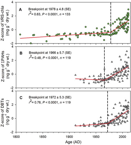
Long-term trends in PAC deposition (Kurek et al. 2013) provided further evidence that pollutants were being transported away from OS operations. As shown in Figure 2, dating the layers in sediment cores showed that deposition and accumulation of PACs in the environment started to increase around 1970, congruent with the time that oil sands industrial activity and oil production began to increase. There has been a clear trend of increasing PACs since that time.

Figure 2. Long-term trend in PACs in lake sediment cores sampled from the five to six lakes proximate to major oil sands operations. Data represented as standardized values (Z scores). Upper graph (A) shows a change in visible reflectance spectroscopy (VRS) of chlorophyll (indicative of productivity). Middle graph (B) shows the total polycyclic aromatic hydrocarbon (PAH) concentrations, and the bottom graph (C) shows the total dibenzothiophene (DBT) concentrations. The lines are from two segmented, piecewise linear regression models to identify the timings of breakpoints (from Kurek et al. 2013).

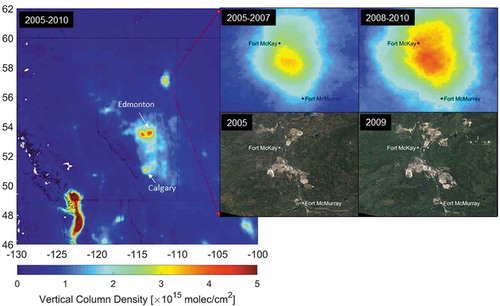
Enhanced air monitoring using passive samplers undertaken by the Wood Buffalo Environmental Association (WBEA) found that pollutants related to acid deposition (i.e., sulfur dioxide [SO₂], nitrogen dioxide [NO₂], and nitric acid [HNO₃]) were moving from source areas to natural ecosystems (Hsu 2013). The RSC report identified monitoring results even farther downwind in Saskatchewan, and although there was no evidence of OS-related SO₂ in the available data, NO₂ was elevated up to 150 km east of the provincial border with Alberta (The Royal Society of Canada 2010). Satellite products derived from multiple years of overpasses (Figure 3) show that NO₂ is elevated over a large area in the OS region. Comparison of images across time revealed the magnitude of the increase in NO₂ concentrations over the northern part of the near-surface deposit region and the size of the area impacted (see also Figure S3.5).

Figure 3. Increase in average column nitrogen dioxide (NO₂) over the oil sands region between 2005–2007 and 2008–2010 observed from the “OMI satellite.” Upper right images show spatial patterns in column NO₂, and the lower accompanying images show the growth in development between 2005 and 2009 from Landsat. The background image is 2005–2010 average column NO₂ from OMI over northwestern United States and western Canada.

(adapted from McLinden et al. 2012)

WBEA was and continues to be responsible for compliance-oriented monitoring in the region. With support from the OS industries, WBEA has also established a range of research programs designed to help close the knowledge gaps relevant to studying the fate and impact of OS air pollutant emissions (Wood Buffalo Environmental Association, Canada 2018). Early results of this work are summarized by Percy (2012). Of relevance here are the measurements of metals and PACs in lichen collected at multiple locations and distances from the emission sources (Studabaker et al. 2012). This early report again demonstrated that air pollutants were being deposited into the environment downwind of the OS activities.

Atmospheric models have frequently been applied to the OS area for a variety of purposes (e.g., Jung and Chang 2012), but particularly for air quality management (Davies 2012). Although much modeling work was undoubtedly done to assess the impacts of specific new sources as part of the development approvals process, larger-scale models have provided estimates of the regional transport and fate of emissions from the OS emissions. They demonstrate that primary air emissions and/or their secondary products can move and be deposited far downwind. During the development of the ECCC-JOSM Air Component science plan, deposition estimates were produced from ECCC’s modeling system and compared with the available aquatic and terrestrial critical load maps (Aherne 2011). These analyses suggested that critical loads were potentially being exceeded (Figure S1.2), especially in the acid-sensitive areas located in northern Saskatchewan.

Given clear evidence of the movement of a variety of air pollutants into the environment “beyond the fence lines,” the critical questions were (and remain) the following: Are effects occurring? If yes, how significant are they? Can they be attributed to air pollutants from the OS? If no, given the long-term accumulation of deposited pollutants in the ecosystems, and the expected growth in developments in the OS, are significant effects expected in the future? And finally, is the monitoring system in place adequate for early detection of these effects to ensure that they can be managed and possibly mitigated? In terms of this latter question, the perspectives of the EC and RSC panels were that the monitoring system needed improvement. Also, an important concept for future monitoring, as expressed by the EC Panel, and recognized in implementing JOSM, was that it needs to be adaptive (e.g., able to change to address new evidence or monitoring needs in a timely manner).

The challenge of measuring ecosystem effects

Although the origin of potentially harmful contaminants in the ecosystem could be direct release or contaminated groundwater seepage to the watershed or possibly spillage onto land areas, atmospheric deposition is a well-documented pathway in the OS, as discussed above. However, once taken up by the biota, the original pathway is difficult to discern, and measuring and interpreting the effects of these exposures represents an ongoing challenge.

Given what science is beginning to appreciate about low-dose effects and the effects of combinations of stressors (Dziedek et al. 2016; Gerner et al. 2017; Liess et al. 2016), it is uncertain whether single-pollutant or -stressor guidelines can be sufficient, even if set with precautionary margins, to serve the desired cumulative effects management approach. Nonetheless, applying single-indicator measures requires an evaluation process (The Royal Society of Canada 2010). For toxics in aquatic ecosystems, as an example, this generally involves chemical and biological measurements to characterize water quality using best available criteria and setting effects-based objectives in the context of background conditions (e.g., specific to the Lower Athabasca River). To determine whether there is unacceptable risk, thresholds or critical effect sizes (CESs) for ecosystem safety are needed. Ideally, biologically relevant CESs should be defined a priori and should consider the type and magnitude of change that is likely to be of concern (Munkittrick et al. 2009). What is traditionally available, in Canada at least, are guidelines set by government agencies such as the Canadian Council for Ministers of the Environment (CCME), which has established guidelines for surface water quality (CCME, Canada 1999). U.S. Environmental Protection Agency (EPA) guidelines also support evaluation of the potential level of risk (U. S. EPA 2019a).

There are numerous aspects of ecosystems that could be monitored for evidence of potential impacts and that need to be considered to meet the RSC’s recommendation regarding cumulative effects management. In general, air pollutants that can elicit an ecosystem or biotic response through deposition are classified into the following categories: acidifying pollutants, eutrophying pollutants, trace elements, and polycyclic aromatic compounds (PACs) (Wright et al. 2018). In order to monitor these, and investigate potential impacts and “leading-edge” indicators of ecosystem effects, certain indicators or biotic response measures have been examined and/or proposed. For instance, some examples of ecosystem effect or health indicators that may be relevant in the OS include critical load, critical level, acid neutralizing capacity, ground-level ozone exposure indices (Accumulated Ozone exposure over a Threshold of 40 ppb [AOT40], The sum of hourly ozone concentrations equal to or greater than 60 ppb over the daylight period 08:00 – 19:59 [SUM60]), eutrophic load, nitrogen saturation, algae bloom, acidity of ombrotrophic bogs, biodiversity of plants or animals, forest resilience, toxicity to biota, chemical burden in animal tissues and embryos, reproductive success of animals, animal stress and death, human health arising from multiple exposure routes, and human stress (fear of direct pollutant effects or of food security and food and water safety). These examples largely involve biological (e.g., biodiversity, health of animal and vegetation species and humans) and chemical-physical (e.g., atmospheric deposition amounts, water chemistry) indicators and do not reflect potential systems-based indicators (e.g., adaptive capacity, resilience) and traditional ecological knowledge (TEK).

In terms of systems-based indicators, combinations of the indicators in the example list may provide insight into the state of the whole system, a concept that could be developed in the future. Monitoring forest health represents a form of a systems-based indicator. Thus, the Terrestrial Environmental Effects Monitoring (TEEM) program operated by WBEA (Jacques and Legge 2012; Percy, Maynard, and Legge 2012) strives to obtain a wide range of measures at multiple forest plots, including atmospheric inputs and is a valuable resource for tracking change over the long term, which may then trigger follow-up to identify potential causes. TEK must also be included in an adaptive monitoring program to provide insight on ecosystem health. As an example, WBEA has been working with local indigenous harvesters to examine concerns regarding the health of local wild berry plants and safety issues regarding the consumption of wild berries. Perceptions of appearance and taste are being explored with data on chemical composition and potential contaminant load (Wood Buffalo Environmental Association, Canada 2019).

In terms of the biological and chemical-physical indicators, clear criteria regarding thresholds of effects are difficult to determine and may be outdated. Chemical-physical indicators exist to provide an easier-to-monitor and early warning approach for tracking biological response (i.e., the chemical-physical and biological response indicators are correlated but are not the biological response per se). Munkittrick and Arciszewski (2017) considered the case of changes in PACs in sediment cores in the Cold Lake, Alberta, area as reported by Korosi et al. (2016) They pointed out that as our capacity to detect any change advances, we also require a counterbalance to account for “trivial” change. Their suggestion was that this could be done through an interpretative framework based on contextualization of differences; the goal is to generate meaningful information for environmental monitoring programs and potential actions. A critical part of the proposed framework is data on normal ranges, considering site-specific, local, and regional (distant) levels. Difficulties remain in contextualizing the levels of exposure, complicated by noisy baselines or small changes that are or may be well below expected levels for ecological impact (Willis et al. 2018; Summers et al. 2016). Ideally, such a framework would be developed and would be routinely applied to monitoring data to determine when a change has occurred that is considered “significant” and that warrants further study (Arciszewski et al. 2017a).

Examples of air pollution–related indicators

A critical load is defined as “a quantitative estimate of an exposure to one or more pollutants below which significant harmful effects on specified sensitive elements of the environment do not occur, according to present knowledge” (Nilsson and Grennfelt 1988). A critical level for vegetation is defined as the “concentration, cumulative exposure or cumulative stomatal flux of atmospheric pollutants above which direct adverse effects on sensitive vegetation may occur according to present knowledge” (Convention on Long-Range Transboundary Air Pollution [CLRTAP] 2017). Most of the currently specified critical levels identify a threshold meant to protect a certain percentage of species at a given confidence level, usually set to a level where the impacts will become discernible (e.g., 5–10% damage). However, they are still single-stressor (e.g., ozone) indicators that do not take into account the impact of climate or soil and plant factors associated with ozone uptake. More-detailed calculations that, for instance, estimate the phytotoxic ozone dose (POD) above a given threshold are preferred where possible (CLRTAP 2017).

Internationally recognized procedures for the generation and use of critical level and critical load data have been set out in the United Nations Economic Commission for Europe’s (UNECE) Convention on Long-Range Transboundary Air Pollution (CLRTAP 2017). Development of location-specific critical loads for sulfur and nitrogen deposition that reflect the potential for an ecosystem response or a biological effect required years of monitoring and research on acid deposition and eutrophication. Through this work, exposure models were developed to estimate an ecosystem-specific critical load based upon terrestrial or aquatic ecosystem parameters. For acidifying deposition, these include the Simple Mass Balance (SMB) model for terrestrial ecosystems and the Steady-State Water Chemistry (SSWC) and First-Order Acidity Balance (FAB) models for aquatic ecosystems (CLRTAP 2017). These models are based on the concept of determining the charge balance of ions in soil water (terrestrial ecosystems) or within lakes (aquatic ecosystems); exceedances are thus with respect to the extent to which strong anion deposition that can’t be buffered by cations present in and/or being deposited to the ecosystem, is above an anion threshold, which will depend on the sensitive plant or animal species within the ecosystem. It should be noted that these UNECE-recommended models for critical loads are “steady-state” models; they only indicate that ecosystem damage at a given total deposition level (or calibrated to a specific wet deposition amount) will occur at some point from the present time to some point in the future. They do not provide the time frame to when the effects will become noticeable (which could potentially be anywhere from an immediate impact to years or even centuries in the future). This is a drawback of the methodology, but exceedances of critical loads have nevertheless been considered, at least in Europe, sufficient cause to enact legislation designed to reduce acidifying emissions.

Dynamic critical load modeling has been attempted as another approach with the potential to estimate the time-to-effect for critical load exceedances; these models were originally intended as a means to estimate the time-to-recovery of damaged ecosystems (CLRTAP 2017). However, the CLRTAP protocols stress the dependence of dynamic models on very accurate local data, and recent work in Canada suggests that dynamic models are so poorly constrained by lack of this information to preclude their use for policy decisions relating to acidifying deposition (Whitfield and Watmough 2015). Variations on the CLRTAP (2017) acidifying deposition critical load estimating procedures and formulae have been constructed, usually employing simplifying assumptions and/or local information. An example is the protocol agreed upon by the New England Governors–Eastern Canadian Premiers (NEG-ECP 2001; Ouimet 2005) that has been used in the past to create Canada-wide acidifying deposition critical load data sets (Aherne and Posch 2013; Carou et al. 2008; Jeffries et al. 2010). These data are used in the context of the OS later in this review.

Critical loads may also be calculated for the deposition of toxic heavy metals (cadmium, lead, and mercury) (CLRTAP 2017). As for acidifying deposition, critical loads for toxic metals are calculated based on the receiving ecosystem (terrestrial or aquatic), but are further subdivided into the metals’ impact on human health versus ecosystem functioning. The human health impacts result from uptake of metals into human food sources and groundwater (metal content in food/fodder crops, grass, and animal products, the total metal content in soil water below the rooting zone, and the metal concentration in fish). The impacts on ecosystem functioning include the free metal ion concentration in soil solution (impacts on invertebrates, plants, and soil microorganisms), the total metal concentrations in forest humus (impacts on invertebrates and microorganism impacts), and the total metal concentration in freshwater (impacts on the food chain, from algae through to top predators). As with acidifying pollutants, exceedances for metal critical loads only indicate that at this estimated critical input flux rates, harmful effects will eventually occur, but not when they will occur. Metal critical load calculations have additional constraints or limiting factors: (1) they may not be calculated for locations where more water is lost than gained (preventing soil leaching and leading to the accumulation of salts and high pH), and for soils with reducing conditions such as wetlands; and (2) they do not include weathering inputs of metals (which are usually of low relevance and are difficult to calculate accurately but may influence metal levels at locations where the geological content of metals is high). Interactions between heavy metals and acidity, whether when in the atmosphere (i.e., on aerosols) or upon deposition, are also challenging to consider but may be important given that acids can convert metals into more bioavailable forms (e.g., water soluble).

Even though reasonably well developed, there remain uncertainties and data limitations with critical loads and levels, as highlighted above. In terms of nitrogen deposition, before an ecosystem is declared to be in a state of nitrogen saturation (Earl, Valett, and Webster 2006; Jung and Chang 2012) that can lead to greater risk of acidification, there are increases in nutrient load or eutrophic load (Smith, Tilman, and Nekola 1999). Beneficial to some plant and tree species and not to others, shifts in plant success and biodiversity can occur, disrupting the natural state (Kwak, Chang, and Naeth 2018), which may require a long period of time to reverse. It is difficult to determine the level of perturbation that is acceptable because it is happening over a continuum and the form of the nitrogen (e.g., reduced, oxidized, or organic), and interactions with base cations, also has critical roles such that there is high diversity in the level of nitrogen sensitivity among ecosystems (Bobbink et al. 2010). Excess nutrients can also have an impact on the allocation of belowground resources (Varma, Catherin, and Sankaran 2018) such as development of root systems (Majdi and Kangas 1997), which may increase vulnerability or resilience to other stressors such as frost, drought, fire, and wind damage (Bobbink et al. 2010). Thus, assessing and projecting the impacts of nitrogen deposition and setting a nutrient nitrogen critical load for the OS region remains challenging (Murray, Whitfield, and Watmough 2017). Similarly, in regard to fertilization (Mullan-Boudreau et al. 2017) or neutralization of acidity in bogs due to input of basic material (e.g., dust from soil erosion), an acceptable amount of decrease in acidity is challenging to determine. Setting thresholds for nutrient loads in aquatic ecosystems (eutrophication) is also challenging given the variability among ecosystems. However, within certain types of environments, critical loads have been established and in some cases an unacceptable point (“threshold”) can be obvious because an undesirable outcome such as excess algae is highly visible.

Challenges in setting thresholds

Although thresholds or critical loads for some heavy metals exist, there is less information on toxicity thresholds based upon the levels of chemicals measured within biota, and there is variability among species. For overall ecosystem protection, this necessitates identification of sentinel species, which could be a plant or animal in any ecosystem (Cruz-Martinez and Smits 2012). Species selection criteria include feasibility, reproducibility, sensitivity, ability for laboratory validation, capability for long-term monitoring, noninvasiveness or nonlethality, ability to set/measure an effects-based threshold, and cost-effectiveness.

For a selected sentinel species, death (e.g., the “canary in a coal mine” concept) is an obvious threshold, but given the availability of different assessment methods and the sensitivity of modern analytical equipment, it is possible to use measures not based on lethality; new monitoring methods continue to change what is possible to measure and observe. Although contaminant load in a range of species has been used extensively, such as mercury levels in fish or colonial waterbird eggs (Campbell et al. 2013; Evans and Talbot 2012) and/or persistent organic pollutants (POPs) in mammals (Metcalfe 2012), laboratory-based analytical measures are becoming more precise. Metabolites in animal blood or tissue, gene expression measures (Gagné et al. 2012; Marentette et al. 2017; Simmons and Sherry 2016), and epigenetic changes (Brander, Biales, and Connon 2017) can be measured and can show evidence of change before the animal’s health and survival are compromised. Other cellular approaches extending from macroscale measures of organs (liver, gonads, thyroid) and immune measures (e.g., Gagné et al. 2017) to telomere dynamics (Moller et al. 2018) are also available or being explored. These cellular or molecular markers may also respond in a dose-dependent manner, with or without an apparent threshold.

Much like particulate air pollution effects in humans, with no discernible threshold in relation to premature mortality and an increasing number of preclinical measures, the appropriate safe threshold for some indicators and most molecular markers of biological effects in nature (i.e., wild animals) remains unclear. This is even more complicated in the context of the challenge of chronic, low-dose exposure, which is an ongoing process occurring in the OS. Precaution, regular reassessment, and continuous improvement is the prudent approach. Ultimately, indicators based upon metabolomics, proteomics, epigenomics, etc., may be the preferred approach given that tracking single chemicals is not fully reflective of the mixtures that occur in reality. Bradley et al. (2019) recently assessed multiple indicators of cumulative contaminant effects (hazard) for in-stream biota, including in silico approaches such as ToxCast (EPA 2017). High-throughput methods for wildlife based on gene arrays and microarrays are also being developed. Bradley et al. (2019) point out that given the 80,000+ parent compounds estimated to be in current use globally and the “inestimable chemical-space of potential metabolites and degradates” from these compounds, toxicity assessment remains a major challenge.

The adverse outcome pathway (AOP) is a conceptual framework for organizing existing knowledge concerning biologically plausible, and empirically supported, links between molecular-level perturbation of a biological system and an adverse outcome at a level of biological organization of regulatory relevance (Villeneuve et al. 2014). This resembles the exposome concept (Wild 2012) being explored to improve understanding of how environmental factors lead to chronic disease in humans (Rappaport and Smith 2010; Wild 2012). To be repeatable and adaptable to multiple types of ecosystems (or individuals), AOPs must be developed in accordance with a consistent set of core principles (Villeneuve et al. 2014).

Potential of remote sensing

The indicators discussed above require tracking effects “on the ground,” through repeated monitoring. The exception might be using atmospheric models to identify areas of critical load exceedances and setting new emission regulations so that future deposition is deemed acceptably below exceedance levels. However, field observations are still necessary to verify that the desired outcomes are being achieved. The cost of this tracking or monitoring may be considerable, especially in remote yet sensitive areas, and could benefit from more efficient approaches. Remote sensing is receiving attention in this regard (Andrew, Wulder, and Nelson 2014; De Araujo Barbosa, Atkinson, and Dearing 2015; Kerr and Ostrovsky 2003; Knox et al. 2013; Sioris et al. 2018). If satellite observations could be used for early warnings of change, then there could be cost savings while also increasing the size of the area possible to have under surveillance. Mapping ecosystem services, including in natural wetlands, is one potential possibility for this information (Radeva, Nedkov, and Dancheva 2018; Zergaw-Ayanu et al. 2012). For satellite observations, sufficient temporal, spatial, and spectral resolutions are needed. Also, for such indices to be sensitive to important characteristics of the ecosystems and their functional attributes, satellite data need to provide the ability to track phenological changes and understand interannual variability of ecosystem processes (Paruelo et al. 2016). Although satellites or other types of remote sensing (e.g., from aircraft-based aerial surveys) are not capable of providing all that is needed for cumulative effects monitoring, including the need for strong empirical data allowing early detection of ecological change (Lindenmayera et al. 2010), they could play a valuable role in remote areas such as the OS.

Main findings from the ECCC Air Component program of JOSM

Four overarching questions were posed to guide scientific activities toward meeting the Air Component objectives:

1. What is being emitted from the oil sands operations, how much, and where?

2. What is the atmospheric fate (transport, transformation, deposition) of oil sands emissions?

3. What are the impacts of oil sands operations on ecosystem and human health?

4. What additional impacts on ecosystem health and human exposure are predicted as a result of anticipated future changes in oil sands development?

Focused studies involving short- and long-term field measurements (ground and airborne) were undertaken to answer the first two questions and to support water and wildlife research in answering the third question. In addition to these monitoring and research activities, an approach to integrate the information gathered from the ambient and emission monitoring using air quality models, as well as satellite-based information, was included in the Integrated Monitoring Plan (Environment Canada 2011). Information from air quality models provide essential input to ecosystem- and health-based models, ultimately providing insight into the potential human and ecosystem health impacts from the OS (fourth question) (Environment Canada 2011).

Improving understanding of emissions to the atmosphere

Among the complex open-pit mining and oil extraction processes in the surface mining facilities of the OS, pollutants are mainly emitted from five processes: (1) exhaust from off-road vehicles used for removal of the surface overburden and for excavation and transportation of the oil sands ores to an extraction plant; (2) ore processing at the extraction and upgrading plants, resulting in stack emissions; (3) fugitive volatile organic compound (VOC) emissions from mine faces, tailings ponds, and extraction plants and volatilization of fuels used for industrial activities and vehicles; (4) fugitive dust emissions from surface disturbances by the large fleet of mining and transportation vehicles; and (5) wind-blown dust emissions from open surfaces such as mine faces and tailings pond periphery beaches. These emissions are superimposed on other emissions, such as on-road vehicle exhaust, wildfires, residential wood combustion, and other industries (e.g., cement, construction), several of which are engendered by population growth owing to OS employment.

The National Air Pollutant Release Inventory (NPRI) and the complementary Air Pollutant Emissions Inventory (APEI) contain annual emission estimates for the region. NPRI (Government of Canada, Canada 2019a) includes data reported by facilities on releases, disposals, and recycling of over 300 pollutants. NPRI collects data from over 9000 industrial facilities nationwide, including the OS, that meet specified reporting criteria and whose emissions meet or exceed reporting thresholds for NPRI-listed substances. The APEI expands on the official, annually reported data, quantifying emissions from a range of other important sources (e.g., motor vehicles, agricultural activities, natural and open sources, etc.) for several common air pollutants, by province/territory, and for all of Canada (Government of Canada, Canada 2019b). According to the 2013 NPRI, which was the year available at the start of the Air Component program, emissions from Alberta’s OS sector accounted for 61%, 34%, and 14% of the provincial total reported VOC, SO₂, and nitrogen oxide (NO_x) emissions, respectively. The OS sector was also a large source of particulate matter (PM or total PM [TPM]) and carbon monoxide (CO) emissions in 2013.

NPRI specifies reporting thresholds for “listed substances,” that extends beyond the criteria air contaminants (CACs) and includes range of VOCs such as benzene, toluene, ethylbenzene, and xylenes (BTEX) and some polycyclic aromatic hydrocarbons (PAHs) (Li et al. 2017). Given the complexity of the OS processes that produce atmospheric emissions of primary pollutants and the potential for secondary formation of other pollutants, it was suspected that other, “unknown” or “unmeasured” pollutants would be present in the air over and downwind of the region. Therefore, a key part of addressing the first question (“What is emitted”) was the need for more detailed ambient measurements from the air and the ground. These new data were expected to help determine what other pollutants might be important to understand in the context of emission reporting, future long-term monitoring needs, and potential for ecosystem and human health effects.

The NPRI and APEI have traditionally been used for the fine-scale air quality monitoring and modeling necessary to characterize the air emission sources and their associated impact on air quality. However, in the development of the Air Component program, it was recognized that this inventory did not contain the multipollutant and multiscale air quality information at the finer spatial and temporal scales necessary to satisfy the JOSM objectives. Therefore, a review of 10 available national, provincial, and subprovincial emission inventories in 2012 (Alberta Environment and Sustainable Resource Development 2013) was undertaken, leading to a new hybrid inventory (JOSM, Canada 2016; Zhang et al. 2018). The hybrid inventory, which also included better representation of spatial and temporal emission patterns, was expected to improve results from the daily air quality model runs. These runs commenced in 2013 for the first intensive field study in August and September of that year and have continued since that time (Figure S3.3).

Uncertainties in the OS emissions

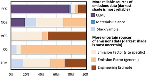
The criteria air contaminant (CAC) emissions from the OS (including NO_x, VOCs, SO₂, ammonia [NH₃], CO, and PM with aerodynamic diameters <2.5 and <10 μm [PM_2.5 and PM₁₀]) have different degrees of uncertainties and, conversely, reliabilities (Alberta Environment and Parks 2016). As shown in Figure 4 the most reliable emission data (i.e., in the hybrid inventory) are for SO₂, with about 80% of the emissions monitored by continuous emission monitoring systems (CEMS), but also with significant contributions estimated through the use of site-specific and generic emission factors (EFs). The latter would have larger uncertainties compared with those obtained through CEMS, even though the CEMS data may also need external evaluation. For NO_x, the fraction of emissions monitored by CEMS drops substantially to ~30%, and the majority of the emissions were estimated using site-specific or generic EFs. For VOCs, there were few actual emission measurements; application of site-specific EFs accounted for about 20% of the estimated emissions, whereas the remaining emissions were derived from generic EFs or engineering judgment. These emission reports were thus expected to have much higher degrees of uncertainty compared with those for SO₂. The same can be said about CO and PM emissions from the oil sands surface mining facilities. Current knowledge on PM emissions was reviewed recently by Xing and Du (Xing and Du 2017).

Figure 4. Sources of emission data for criteria air contaminants from the oil sands facilities. Results are summarized from the Alberta Environment Sustainable Resource Development (AESRD; now part of Alberta Environment and Parks) industrial survey on quantification of criteria air contaminant emissions from nonconventional oil and gas sectors (JOSM 2016).

Recognizing the likelihood of emission uncertainties, the hybrid emission data were updated through use of multiple sources of information (Zhang et al. 2018). These included, for example, new versions of NPRI and APEI, measurements from CEMS attached to 17 stacks at four OS mining facilities for the 2013 field-study period, and daily reports of SO₂ emissions during a 1-week period in August 2013 when the Canadian Natural Resources Ltd. (CNRL) Horizon facility experienced abnormal operating conditions and the aircraft was conducting emission evaluation flights. Other key limitations of prior inventories, highlighted in Zhang et al. (2018), that have been systematically assessed and improved, where possible, include (1) the lumping of all stack emissions under 50 m with surface-level fugitive emissions and thus treated as surface releases (Environment Canada, Canada 2016) without consideration of plume rise; (2) the lack of spatial allocation of surface-level fugitive VOC emissions, which were reported to NPRI as facility-total emissions without differentiation between source type (e.g., mine faces, tailings ponds, and extraction and upgrading plants); (3) out-of-date vegetation fields used for biogenic emissions such that much of the area now being mined was still being treated as forest; (4) failure to treat the tailings ponds present in the mining facilities as water-covered even though by 2013 the tailings ponds in the OS region covered an area of about 180 km²; (5) exclusion of some of the available CEMS data (hourly SO₂ and NO_x emissions and measured stack volume flow rates and exit temperatures) given that such data exist for 100 stacks at 33 facilities with relatively large SO₂ or NO_x emissions.

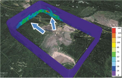
Despite the initial improvements in the emission estimates, the lack of independent evaluation and emission determination continued to contribute to uncertainty. Thus, a key component of the aircraft measurement campaign was validation of the reported CAC emissions, as well as quantification of the emissions for a range of other compounds. From the aircraft it was possible to obtain a large number of VOC and chemical speciation profiles from each surface mining facility (Li et al. 2017), thereby targeting one of the main uncertainties for one of the major pollutant classes associated with the OS. The instrument package onboard the aircraft also provided the opportunity to estimate facility-total PM emissions across a large size range of particles (0.6–20 μm in diameter). Figure 5 shows an example of aircraft observations of PM_2.5 throughout a complete box flight around a facility. These box flights (Figure S3.1) were a key part of the aircraft campaign in August–September 2013 because they enabled observation-based estimates of short-term emission rates for multiple pollutants.

Figure 5. Interpolated observations of PM2.5 obtained from the box aircraft flight around the Syncrude Mildred Lake (SML) facility during flight F12 on August 24, 2013. The arrows show the mean wind direction at different flight altitudes corresponding to the maximum plume concentrations on the box walls. Plumes for PM2.5 can be seen moving northward away from the facility, and there appears to be multiple sources related to the plants and surface mining activities.

Validation of emissions from aircraft studies

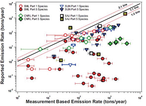
Li et al. (2017) used the Top-down Emission Rate Retrieval Algorithm (TERRA) (Gordon et al. 2015) (see Section S3.1.1 of the supplemental material) with aircraft-based measurements to estimate facility-total emissions for several VOCs. They found that the values of the summed VOC emissions, quantified for four of the key facilities in the surface mining region: Syncrude Mildred Lake (SML), Suncor Millenium and Steepbank (SUN), Canadian Natural Resources Ltd Horizon (CNRL), and Shell Albian Sands and Jackpine (SAJ)—now operated by CNRL, were factors of 2.0 ± 0.6, 3.1 ± 1.1, 4.5 ± 1.5, and 4.1 ± 1.6 higher, respectively, when scaled to annual totals compared with the data contained in the NPRI.

Figure 6 shows differences in measured (TERRA) versus reported (NPRI) annualized emission estimates for 93 separate VOC species included in annual emission reports (totals among the four facilities) grouped by the reporting categories (i.e., Part 1, Part 5) of interest to NPRI. Only 11 of the 93 species had aircraft-observed annualized emissions that were similar to reported values, whereas 82 species had lower reported emissions than aircraft-based emission estimates (TERRA) by a factor of 2 to 27,800 (Li et al. 2017). Looking closely at some specific species, the total aromatic emission rates were 9.7 ± 1.5, 7.9 ± 0.5, 2.1 ± 0.3, 1.5 ± 0.2, 0.53 ± 0.06, and 0.15 ± 0.02 tons day⁻¹ at SML, SUN, CNRL, SAJ, Syncrude Aurora (SAU), and Imperial Kearl Lake (IKL), respectively. These quantities were composed of similar proportions of aromatics at SML, SUN, and CNRL, but different proportions at SAJ, SAU, and IKL. The higher than previously estimated aromatic emission rates, coupled with the similarities in the aromatic compositions, are thought to reflect the naphtha-type solvents used in the bitumen extraction process at SML, SUN, and CNRL. Conversely, at SAJ, SAU, and IKL, paraffinic solvents are used (Alberta Environment and Parks [AEP] 2016), and the lower aromatic emission rates detected for these facilities is consistent with this knowledge. Large contributions from alkanes, which peak between C₄ and C₈, were measured for most of the facilities, and this reflects the use of naphtha and paraffinic solvents used in bitumen-sand-water separation. Naphtha solvents have higher-carbon alkanes (>C₆) and a high aromatic content, whereas paraffinic hydrocarbons contain carbon numbers around C₆ as the effective ingredients (AEP 2016; Davies 2012). The aircraft and ground data were able to detect these differences, suggesting that VOC ratios may be useful as near-field tracers associated with each facility.

Figure 6. Comparison of 2013 emission rates for the individual species reported to the Canadian National Pollutant Release Inventory (NPRI) with the measurement-based emission rates for the same species. Each dot represents a reported species under either Part 1 or Part 5 of the NPRI reporting requirements. The horizontal bars represent the uncertainty range of the measurement-based emission rates (Li et al. 2017).

PM emissions from the facilities originate mainly from four major source categories: (1) emissions from plant stacks; (2) tailpipe emissions from the off-road mining fleet; (3) fugitive dust originating from various mining and transportation activities, such as excavation of oil sands ore, loading and unloading trucks, and wheel abrasion of surfaces by off-road vehicles; and (4) wind-blown dust. Emission data from plant stacks and fugitive dust source categories are available in NPRI, whereas emissions from tailpipe emissions are provided from other sources (APEI). Although these emissions are uncertain, the most significant uncertainty in the PM emission inventories for the OS region is associated with fugitive dust.

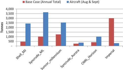
TERRA results have been reported for PM_2.5 (Zhang et al. 2018), and, as shown in Figure 7, the reported base case PM_2.5 emissions are considerably less than the estimates derived from the aircraft measurements for five of the six facilities studied. Although these discrepancies are for PM_2.5, Figure S3.4 shows that 65–95% of PM_2.5 emissions are in PM size bin 8 (diameter range from 1.28 to 2.56 μm), implying that the majority of the PM_2.5 mass emissions are from fugitive dust area sources (Eldering and Cass 1996), either from dust kicked up by off-road mining vehicles or from wind-blown dust. It is reasonable to expect that this increase in mass toward the larger PM_2.5 sizes continues into larger sizes, which are likely associated with fugitive dust emissions. This has implications for acidic deposition given that in these sizes basic material (e.g., calcium [Ca]) is typically present (Wang et al. 2015; Zhang et al. 2018). Given the presence of petroleum coke (petcoke) stockpiles at the facilities where bitumen is upgraded, there is the potential that these large particles also contain PACs.

Figure 7. Comparison of PM_2.5 emissions between base case annual emissions obtained from all available bottom-up emission inventory information and the aircraft-observation-based (top-down) estimates for the two summer months (August and September 2013) for the six oil sands mining facilities (Zhang et al. 2018).

In addition to potential differences seen through direct comparison (i.e., Figure 7), there has often been a discrepancy between initial inventory estimates of primary PM emissions and the amount of PM actually detected in the atmosphere downwind (i.e., “transportable fraction”). This tends to depend on the type of land cover and indicates that a fraction of the emitted PM is deposited locally and thus does not escape into the boundary layer or free troposphere for transport downwind (Pace 2005). The range of uncertainty associated with the estimate of the transportable fraction is high, and TERRA estimates in the OS region may help constrain the value of this parameter.

In terms of PM chemical constituents, total black carbon (BC) emissions from the OS surface mining facilities were estimated using the hourly emission rates (TERRA) to be 707 ± 117 tons yr⁻¹. The total annual BC emissions reported to the UNECE by ECCC (2016) are similar to these measurements, lending some confidence to both results. However, the relative contributions of off-road vehicles versus stacks in the UNECE report differ from the TERRA estimates, with the latter attributing the majority of BC emission to off-road vehicles versus only 50% for the UNECE report. These differences suggest that the UNECE reported total amount, which is derived using the standard approach (i.e., from PM_2.5 mass emission estimates for the oil sands surface mining facilities in conjunction with the EPA SPECIATE database [EPA 2014] BC/PM_2.5 fractions [Cheng et al. 2019]) is reasonably accurate, but differences by source category suggest a potential need for improvements.

Low-molecular-weight organic acids (LMWOAs) and isocyanic acid (HNCO) had never been reported for the OS, or for most other sources in Canada or globally. They are both products of secondary formation in the atmosphere but are also directly emitted. The transportation sector is an important source of HNCO (Brady et al. 2014; Wentzell et al. 2013; Wren et al. 2018), and emission rates were estimated from the aircraft measurements to be 2.2 ± 0.8 kg hr⁻¹ from SUN, followed by that from the SML facility of 1.5 ± 0.5 kg hr⁻¹. Figures S3.2a and S3.2b show that by tracking a specific integrated plume downwind, increases in HNCO and LMWOAs can be observed (Liggio et al. 2017). Additionally, for HNCO, there is alignment of the plume emanating from SML and the location of active open-pit mining, which is consistent with the expectation of the source being the off-road heavy-duty diesel fleet. Isocyanates, of which HNCO is the simplest stable and volatile species, have recently been classified as being in the highest inhalation toxicological potency class in an assessment of 296 inhalable species of concern (Schüürmann et al. 2016).

LMWOA emissions (Figure S3.2a) for the SUN, SML, SAU, SAJ, CNRL, and IKL facilities were estimated to be 162 ± 22, 108 ± 15, 45 ± 6, 56 ± 8, 60 ± 8, and 19 ± 3 kg hr⁻¹, respectively, or approximately 12 tons day⁻¹ of primary LMWOAs (Liggio et al. 2017). From the atmospheric chemical process perspective, LMWOAs could be contributors to precipitation acidity and ionic balance, particularly in remote areas (Khare et al. 1999; Stavrakou et al. 2012). Although important in their own right, their relative contribution to acidic deposition could become more important if anthropogenic NO_x and SO_x emissions decrease. LMWOAs are also key participants in the aqueous-phase chemistry of clouds and contribute to secondary organic aerosol formation through various reactions within the aqueous portion of the particle phase (Carlton et al. 2007; Ervens et al. 2004; Lim et al. 2010). Furthermore, since organic acids are also formed in photochemical reactions, their measurements serve as indicators of atmospheric transformation processes. Thus, measurements of LMWOAs can help evaluate the Global Environmental Multiscale–Modeling Air-quality and Chemistry model (GEM-MACH), specifically the chemical mechanisms within the model. From an environmental health perspective, deposition of LMWOAs may have ecosystem impacts, as they have been shown to be toxic to various marine invertebrates (Staples et al. 2000; Sverdrup et al. 2001), phytotoxic (Himanen et al. 2012; Lynch 1977), and interfere with the uptake and mobilization of heavy metals by microbial communities in soils (Menezes-Blackburn et al. 2016; Song et al. 2016). However, studies on the human toxicity of LMWOAs are sparse and the results unclear (Azuma et al. 2016; Rydzynski 1997).

It is important to note some of the limitations in the current emission validation findings derived from the top-down approach. Because of limitations in the minimum aircraft flying altitude, there is larger uncertainty in the emission estimates associated with surface sources; 20% versus elevated stack emissions at about 10% (Gordon et al. 2015). However these uncertainty levels are small compared with those expected for bottom-up inventory estimates from large and complex area sources such as OS facilities.

The largest uncertainty regarding comparison of the top-down results and the reported inventory is potentially due to the limited number of flights around each facility. These were also limited in time (i.e., August–September 2013); thus, the top-down estimates in general needed to be temporally extrapolated for comparison with data in the NPRI and APEI databases. These extrapolations were done with caution, taking into consideration potential uncertainties and with noted caveats (Li et al. 2017). Another limitation is that although TERRA can theoretically be applied to any size volume (i.e., could isolate a single stack), aircraft flights become logistically challenging to capture smaller elements within the OS facilities. Thus, the emission data reported thus far are for mainly whole facilities, recognizing that there is heterogeneity in the emissions across these relatively large areas and that more-resolved measurement would be desirable.

Ground-based measurements have also been analyzed to assess consistency with known emissions. For example, Parajulee and Wania (Parajulee and Wania 2014) suggested that a significant amount of PAH emissions from tailings ponds would be necessary to explain their modeling results. The Galarneau et al. (2014) study of tailings pond water supported this finding, demonstrating that given known water concentrations, there is a potential for PAHs to partition into the air. Harner et al. (2018) also highlighted that potential; in order for the inverse modeling of Parajulee and Wania (2014) to explain the observed ambient concentrations of phenanthrene, pyrene, and benzo[a]pyrene in 2009, their emissions would need to be 2–3 orders of magnitude higher than those reported in the NPRI and APEI databases. More recent emission estimates, also based on inverse modeling, but for a larger amount of ambient monitoring data (Schuster et al. 2015), also concluded that PAH emissions are underestimated (Qiu et al. 2018). This work found that benzothiophene emissions needed to be more than an order of magnitude higher than the currently available estimates in order to explain the observations. Qiu et al. (2018) also estimated what the emissions of alkylated PAHs (alk-PAHs), which are not required to be reported, needed to be to fit the observations: 160 tons yr⁻¹ for C₁-naphthalenes; 130 tons yr⁻¹ for C₂-naphthalenes; 52 tons yr⁻¹ for C₃-naphthalenes; 19 tons yr⁻¹ for C₁-fluorenes; and 35 tons yr⁻¹ for C₁-phenanthracene/anthracenes.

Remote sensing observations are being used extensively to monitor air pollutants over the OS region; SO₂, NO₂, CO, NH₃, methanol (CH₃OH), and formic acid (HCOOH) have been observed from 2004 onward on the Aura satellite. Figure 3 shows how the amount of NO₂ increased over the northern parts of the surface minable region in the late 2000s. The ECCC satellite research has led to improved methods to derive emissions and for retrievals of SO₂ (Fioletov et al. 2017, 2015) and ammonia (Shephard et al. 2015). McLinden et al. (2012) examined the annual trends from 2005 to 2011 and showed that there is good agreement between the trend derived from satellite (vertical column density and area-integrated NO₂ mass) and ground NO₂ observations and bitumen production (Figure S3.5), suggesting that such analyses could provide another independent validation of the reported emissions. Currently, 3-yr running average annual SO₂ emissions from the OS region for 2006–2017 are being analyzed for trends for comparison with the NPRI reports for the same time period (McLinden, personal communication, 2019).

Greenhouse gases (GHG) are generally not a pollutant of interest in regard to long-term ecosystem effects due to deposition/exposure (i.e., the topic of this paper), as is the case for the other pollutants discussed in this section. However, they will contribute to climate change effects. Liggio et al. (2019) report that the aircraft-derived carbon dioxide (CO₂) emissions intensities are, at times, larger than what would be derived using publicly available data in the Greenhouse Gas Reporting Program (GHGRP). The difference in calculation results translates into a potential gap in CO₂ emissions of approximately 17 Mt annually, which could correspond to a 64% increase relative to reported emissions for the four major surface mining operations in the OS. Similarly, methane (CH₄) annual emissions estimated using aircraft hourly emission rates from the five major facilities in the surface mining region was found to be 48 ± 8% higher than that extracted for 2013 from the GHGRP (Baray et al. 2018). These estimates were based upon examination of emissions from mine faces and tailings ponds, which are the major sources of CH₄ on the facilities. Clearly, the discrepancies between the aircraft-based (top-down) emission estimates and the methods used to estimate emissions reported to the GHGRP indicate a need for reconciliation between the bottom-up (used to report to inventories) and top-down estimates.

How do the emissions transform in the atmosphere?—Assessment of changes in pollutants during atmospheric transport

Given the large emissions of volatile organic compounds (VOCs) and other pollutants (e.g., NO_x) from OS sources, it was anticipated that as they are transported away from the source area, they would transform into both gaseous- and particle-phase oxygenated products. Thus, four of the 2013 aircraft flights examined the formation rates of and/or total quantities of secondary organic aerosols (SOAs), particle organic nitrates (pONs), gas-phase low-molecular-weight organic acids (LMWOAs), and isocyanic acid (HNCO) downwind of the OS. In general, ozone levels near and downwind of the OS region are relatively low (i.e., hourly maxima typically less than 60 ppbv) and thus were not a focus of these transformation studies.

SOA formation was hypothesized to be important given that bitumen is composed of lower-volatility hydrocarbons, and open-pit extraction and subsequent processing could release a disproportionately large fraction of SOA precursors (semivolatile organic compounds and intermediate volatility organic compounds [SVOCs/IVOCs]) into the atmosphere. Should even a small amount of the bitumen volatilize during production, there would be a strong potential for SOA formation downwind of the region. However, although oil and gas production and processing, including OS production, were known to be a significant source of VOC emissions (Simpson et al. 2010), SVOC/IVOC emissions were only suspected. Liggio et al. (2016) reported large amounts of SOAs forming downwind (Figure 8) suggestive of such emissions from the OS activities. After correcting for dispersion of the plume as it spread downwind, a 6-fold relative increase in organic aerosol mass (as SOAs) was observed over 4 hr of transport away from the OS facilities. In terms of the amount of SOAs formed, they found that during the summer season of the aircraft flights formation was on the order of 55–101 tons day⁻¹ and likely higher given that SOA formation beyond the last flight screens and at night were not considered. These quantities are comparable to what has been observed forming downwind of major cities (Liggio et al. 2016).

Figure 8. Organic aerosol (OM) observations at varying distances and times downwind from the main oil sands surface mining region (S). The aircraft flew at multiple heights perpendicular to the wind direction to capture the complete plume as it dispersed and transformed. Clear increases in OM after the first transect (A) can be seen by more red, yellow, and green colors in B, C, and D. The yellow text indicates estimates of the amount of secondary organic aerosol (SOA) formed between the separate transects (Liggio et al. 2016).

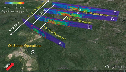
Based upon laboratory experiments, the characteristics of the newly formed SOAs were found to be similar to the hydroxyl (OH) oxidation products of bitumen vapors (Liggio et al. 2016). To determine how much SVOCs/IVOCs would need to be present to explain the observed SOAs, a Lagrangian box model was set up for the OS conditions. This initially only considered the known VOC emissions along with the other primary emissions (e.g., NO_x). However, oxidation products of the speciated alkanes, alkenes, and aromatic hydrocarbons could only explain <6% of the observed SOAs, and adding isoprene and monoterpenes only explained an additional 9% or less. However, by adding into the box at the start of the run 3–4.5 ppbv of bitumen SVOCs/IVOCs, the chemical mechanism and aerosol formation scheme, using realistic physical properties determined in the laboratory (Liggio et al. 2016), was able to simulate the aircraft SOA measurements. After 3 hr, this scheme contributed ~86% of the observed SOAs. Even though 3–4.5 ppbv of IVOCs/SVOCs is small compared with the ~70 ppbv of VOCs observed during the flight at the first pass through the OS plume, the IVOC/SVOC species are the dominant contributor to SOA formation. The existence of significant amounts of IVOCs/SVOCs in the air in the OS region was also verified through ground measurements taken just north of SML (Tokarek et al. 2018). These results highlight the need for additional data on IVOC/SVOC emissions for the OS in order to accurately predict the amount of SOAs and PM_2.5 traveling downwind and potentially accumulating in sensitive ecosystems.

Large amounts of LMWOAs (e.g., formic and acetic acids) were also found to form as the OS emissions moved downwind (Figure S3.2a) (Liggio et al. 2017). Secondary formation rates within 1 photochemical day of the OS were in excess of 180 tons day⁻¹, and the amounts observed were more than an order of magnitude greater than the known/expected primary emissions (Liggio et al. 2017). Based upon the known precursor VOC emissions, Liggio et al. (2017) determined that that amount of LMWOAs formed would require that 50% of the carbon emitted was transformed to organic acids within 1 photochemical day. This is an unusually high effective yield, suggesting the presence of unknown/unmeasured hydrocarbons capable of producing LMWOAs upon oxidation with significant yields. However, current photochemical mechanisms are not able to reproduce the LMWOA observations, suggesting that, similar to SOAs, there is a “missing” precursor. This unknown source would need to account for 54–77% of the observed LMWOAs and is not expected to be related to the oxidation of biogenic species. As for SOAs, IVOCs are suspected to be this source, although through reactions that induce fragmentation of these relatively large carbon molecules (Lambe et al. 2012). In terms of ecosystem impacts, it is presently not clear the extent to which weak acid deposition from LMWOAs to sensitive ecosystems could contribute to critical load exceedances.

Secondary formation of HNCO is known to occur in the atmosphere (Roberts et al. 2014; Wentzell et al. 2013; Woodward-Massey et al. 2014; Zhao et al. 2014a). Laboratory experiments have demonstrated that HNCO is formed photochemically from the OH oxidation of off-road heavy-duty diesel exhaust vapors (Link et al. 2016). Analysis of downwind observations in the OS region (Figure S3.2b) provided two separate estimates of the HNCO formation rate: 116 ± 25 kg hr⁻¹ in one flight and 186 ± 38 kg hr⁻¹ in the other. Relative to the primary emission amount, these secondary amounts, formed after 4 hr, were from a factor of 2 to ≈20 greater than what is estimated to be emitted, although it should be noted that this enhancement in HNCO due to secondary formation in the OS region is based upon conditions in August–September 2013. Atmospheric HNCO production during other seasons is unknown. However, these summertime proportions are much higher than laboratory studies using diesel exhaust (Kang et al. 2007; Link et al. 2016), and the reasons for this large discrepancy are not clear. Something unique with the emissions from the off-road heavy-duty diesel in the OS, or the fuels used, or the levels of NO_x or underestimates in the laboratory experiments due to wall losses of later-generation VOC oxidation products (Lambe et al. 2011) are possible explanations. In terms of implications, current model estimates indicate that potential exposures in close proximity to the facilities (e.g., work camps, Fort McKay) are below the 1000 ppt threshold for potential health effects (Roberts et al. 2011). However, given that HNCO levels are expected to be proportional to OS production because of their link to heavy-duty diesel emissions (Cheng et al. 2018; Liggio et al. 2017), further increases in OS production via surface mining would likely increase HNCO exposures in Fort McMurray and other nearby communities.

As PACs are a diverse class of compounds, their distribution is likely to undergo considerable change as they move from their specific source locations on the OS facilities to downwind areas. Quinones and nitrated compounds are believed to be the dominant end products from these reactions (Arey et al. 1992; Keyte, Harrison, and Lammel 2013; Lundstedt et al. 2007), and these compounds were measured at several ground sites within the surface-mineable region (Harner et al. 2018). Separate measurements of the ambient gas- and particle-phase concentrations of seven unsubstituted PAHs and 19 corresponding quinones at the WBEA site south of Fort McKay, Alberta (AMS13), showed that the unsubstituted PAHs were predominantly found in the gas phase. In contrast, quinones were more abundant in the particle phase (Wnorowski 2017; Wnorowski and Charland 2017). The average 24-hr concentrations were greatest for 2- and 3-ring quinones, average 5.3 ± 7. 8 ng m^–3 (range of 0.1–32.5 ng m^–3); average for 4- and 5-ring species of 0.4 ± 0.6 ng m^–3 (range of 0.1–2.6 ng m^–3); and lowest for 6-ring quinines, average 0.1 ± 0.1 ng m^–3 (range of 0.01–0.3 ng m^–3). These concentrations are of the same order of magnitude as reported elsewhere for industrial sites (Harner et al. 2018). Diurnal measurements showed a higher abundance of quinones during daytime than nighttime, indicating that some PAH sources are linked to daytime local activity and favorable photochemical conditions for the oxidative transformations of quinone precursors. Correlations of quinone and PAH concentrations with colocated primary pollutant measurements (e.g., NO_x) suggested that unsubstituted PAHs originate from primary emission sources associated with OS activities (Wnorowski 2017; Wnorowski and Charland 2017). In contrast, the temperature-dependent formation of the quinones corresponded to a decrease in PAH and NO₂ levels, suggesting gas-phase oxidation of quinone precursors by free radicals (Wnorowski 2017; Wnorowski and Charland 2017).

Given their semivolatile nature, many PACs in the region can be expected to cycle between gas and particle phases depending upon temperature and other atmospheric conditions. This can happen over short (i.e., diurnal) and long (i.e., seasonal) timescales. Hsu et al. (2015) presented evidence of evaporation of PAHs from Lake Gregoire, which may be sufficiently large as to control local atmospheric concentrations in summer, with peak levels occurring in May. They suggest that PAHs that were atmospherically deposited during the winter months may have run off to the lake’s surface waters during snow melt, from which evaporation occurred when temperatures increased in spring. These partitioning processes could have a significant influence on where some PACs accumulate in the environment, in what chemical form, and their atmospheric processing. However, these processes have yet to be explored in a systematic manner in the OS region. A modeling study examining the fate of PAHs relative to trace metals (i.e., inert tracer) around the Sudbury (Ontario, Canada) smelter provides some insight into the impact of these processes (Thuens et al. 2014). As theory would predict, lower-molecular-weight PAHs were observed to have shorter lifetimes than the higher-molecular-weight PAHs. Travel distances in colder winters were more than twice those in the hotter summers, indicative of the longer travel distances possible for particles. Overall, travel distances of up to 500 km were found for the trace metals, whereas they were shorter for the semivolatile PAHs.

Model evaluation and improvement—Toward better tools for integration of information to estimate impacts of OS emissions

The Global Environmental Multiscale–Modeling Air-quality and Chemistry model (GEM-MACH) has been used extensively for applications in the OS region (see Section S3.1.2 of the supplemental material). GEM-MACH (Makar et al. 2015b, 2015a; Moran et al. 2010) stems from a longer history of prediction model development involving the Acid Deposition and Oxidants Model (ADOM), which has its roots in the acid deposition era (Venkatram and Karamchandani 1986), followed by A Unified Regional Atmospheric Modeling System (AURAMS), which was initially developed to incorporate particulate matter in the ECCC’s modeling tools (Brook and Moran 2000; Gong et al. 2006). In parallel to daily GEM-MACH runs based upon the grid and domain shown in Figure S3.3, a number of components in the model have been modified, including emissions, and tested against observations from the aircraft and ground, to determine whether they lead to improved predictions. This iterative process of model evaluation, improvement, and testing is critical given the ongoing role of GEM-MACH in identifying areas of potential concern (e.g., above critical loads) and in a range of other applications in the region (e.g., emission reduction scenarios, air quality forecasting).

Incorporation of observed emission rates from aircraft data

To determine whether GEM-MACH predictions improve through incorporation of the aircraft-based emission estimates (Li et al. 2017), new VOC and size-resolved PM emissions files were created and model sensitivity analyses were conducted (Zhang et al. 2018). In addition to speciating VOCs and PM and adjusting their emission rates to reflect the aircraft observations, spatial allocation of the facility-total emissions to specific locations within the facilities (e.g., stacks, tailings ponds, mine faces) was improved (Figure S3.6). Stroud et al. (2018) found that with the aircraft-based VOC and organic PM emission estimates, changes in the model predictions for the August–September 2013 period was sometimes considerable, particularly based on a comparison of 99th percentiles of aircraft-observed and modeled VOC and organic aerosols (Figure 9). This statistic is a quantitative estimate of whether the model captures the plume maxima mixing ratios, whereas the model median value is more representative of the regional background concentrations. The modeled di/trisubstituted aromatics (AROM) median and 99% percentile mixing ratios were both closer to the aircraft observations. The statistical analysis with the monosubstituted aromatic (TOLU) species showed comparable results (i.e., similar performance with the original and revised emissions).

Figure 9. Comparison of the observed and model histograms of VOC categories simulated by the GEM-MACH model. The first column is from aircraft observations obtained from flights during two summer months (August and September 2013). The second column is from GEM-MACH using the available bottom-up emission inventory information for VOCs and organic aerosol. The third column is model estimates using revised VOC emissions obtained from the aircraft-observation-based (top-down) emission estimates (Li et al. 2017). The 99th percentile values for the different VOC groups and total organic aerosol are displayed in each graph (Stroud et al. 2018).

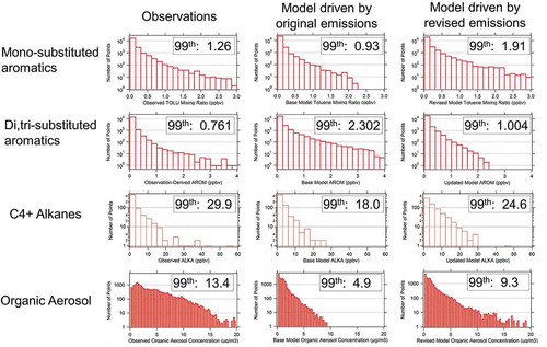
For the C₄₊ alkanes (ALKA), which are emitted in large quantities given their use in bitumen processing (Li et al. 2017), the mean bias and median value were found to be higher with the revised emissions. However, the 99th percentile was closer to the observed value with the revised emissions. In terms of SOA formation, the modeled PM₁ organic aerosol mean bias and root mean square error improved significantly with the revised emissions, although the organic aerosol mean bias still remained negative. One likely cause of the continued underestimate of organic aerosols is insufficient organic aerosol enhancement from secondary formation in the modeled plumes, particularly due to missing contributions from IVOCs/SVOCs (Liggio et al. 2016). Overall, Stroud et al. (2018) concluded that the use of the aircraft estimates of emission rates resulted in comparable or higher, and potentially improved, results compared with predictions based upon the original inventory (i.e., bottom-up inventory) in GEM-MACH.

Increasing resolution in the PM size distribution

Two-bin (size cuts of 0.01, 2.56, and 10.24 μm diameter) and 12-bin (size cuts of 0.01, 0.02, 0.04, 0.08, 0.16, 0.32, 0.64, 1.28, 2.56, 5.12, 10.24, 20.48, and 40.96 μm diameter) particle schemes were implemented in GEM-MACH, and the predicted PM concentrations were compared with surface PM_2.5 observations. The 12-bin version led to improvements, with the mean bias decreasing from −2.6 to −1.7 μg m⁻³ and the fraction of observations within a factor of 2 increased from 0.39 to 0.45 (Akingunola et al. 2018). These observations suggest that a sizeable fraction of particulate underpredictions in 2-bin simulations may be due to poor representation of particle microphysics, despite the sub-binning used in some of the algorithms simulating microphysics processes. Figure 10, which provides information on the PM_2.5 in the region during the August–September 2013 study period, compares the modeled PM_2.5 with the surface observations. The 12-bin scheme did improve predictions, although negative biases for the frequency of low concentration events and positive biases for the frequency of high concentration events were still evident.

Figure 10. Histogram of surface PM_2.5 using Wood Buffalo Environmental Association (WBEA) surface monitoring data (blue), and the 2-bin (red) and 12-bin (purple) configurations of the GEM-MACH model (Akingunola et al. 2018).

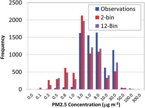
Impact of meteorology on local-scale motions—Vertical and horizontal placement of plumes

GEM-MACH and most comparable models continue to use empirical plume rise formulae based on observations collected between 1969 and 1985 (Briggs 1969, 1975, 1984, 1985). Comparisons between model predictions of the height of SO₂ plumes and the aircraft observations indicated that GEM-MACH had a tendency to underpredict the height of buoyant plumes and overestimate the frequency and intensity of surface fumigation events. To understand possible reasons for this discrepancy and to improve the model, meteorological observations were used to “drive” the standard Briggs plume rise algorithms, and then these and alternative formulations (Gordon et al. 2018) were evaluated using aircraft observations of SO₂ plumes. This confirmed that the plume rise algorithms underestimate plume rise, with 50% or more of the predicted plume heights falling below half of the observed values in the OS region. In addition, computations of plume rise using different sources of meteorological data (aircraft, two tall meteorological towers, and surface-based remote sensing) sometimes resulted in different estimates of plume height, suggesting that plume rise estimates can be influenced by the high degree of spatial heterogeneity in meteorology in the OS region. Meteorological observations close to or at the stacks might therefore be required for observation-based improvements to estimates of plume rise, which can ultimately influence where the emissions are deposited.

Akingunola et al. (2018) compared results from the plume rise algorithms using inputs from GEM-MACH (i.e., as opposed to from meteorological observations) to the aircraft observations. These simulations revealed that the predicted temperature profiles and planetary boundary layer (PBL) heights (key determining factors in plume rise) were different between the locations containing the meteorological observations and the locations of the stacks. That is, the model also revealed the potential for spatial heterogeneity in conditions between meteorological observation locations, again implying that at-stack meteorological observations are needed to obtain optimal results from the plume rise algorithms. Akingunola et al. (2018) also found that once these meteorological differences were taken into account using model predictions at the actual stack locations, a new plume rise estimation methodology that makes use of successive residual buoyancy calculations gave significantly improved results for both plume height and SO₂ concentrations in plumes. However, excessive fumigation relative to observations still occurred at times. This appeared to be related to the meteorological model tending to systematically underpredict the temperatures in the lowest 2 km of the atmosphere, resulting in an overestimation of the temperature gradient and excessive fumigation.

Slight errors in the horizontal direction of advection, which will displace the location of plumes, can result in large errors when predictions and observations are compared. This can be accentuated in more spatially resolved models such that the advantages of the finer resolution, which can be significant for simulating a range of processes, may be difficult to quantify in model diagnostic evaluation (Fox 1981, 1984; Hanha 1988). Russell et al. (2018) presented a new approach to account for this misalignment in their analysis of the potential benefits of a more spatially resolved model (i.e., 1.0 vs. 2.5 km resolution). They accounted for the fact that when the model resolution is relatively low, the plumes spread over a larger cross-sectional distance and wind direction errors have a smaller impact than when model resolution is high and plumes are less spatially distributed (Landers et al. 2010). These techniques have the potential to help evaluate whether improvements to the model, ultimately to predict long-term conditions and undertake emission scenario work, are having the intended benefits. However, for air quality forecasting to provide advanced, short-term warnings (i.e., for location populations), misalignment errors remain problematic, highlighting the ongoing need for more accurate simulations of meteorology. Incorporation of meteorological observations into model forecasts via data assimilation may ultimately be needed to improve air quality forecasting in the OS region.

Two-way air-surface exchange processes—Aircraft and satellite evidence for ammonia bidirectional flux

Concentrations of ammonia (NH₃) measured from the aircraft along with satellite data showed that background NH₃ concentrations in the region were approximately 0.6 ppbv throughout the boundary layer and into the lower troposphere (Shephard et al. 2015). However, initial GEM-MACH simulations underpredicted background NH₃ relative to these observations. Bidirectional fluxes of NH₃, in which natural emissions as well as deposited NH₃ stored within vegetated surfaces is released once concentrations drop below a vegetation-dependent “compensation point” concentration, were tested in GEM-MACH and found to be capable of accounting for the deficit with observations (Whaley et al. 2018b). Bidirectional fluxes may have an impact on net nitrogen deposition, and two-way exchange processes will likely be necessary to better simulate the movement of PACs in the OS region.

Integration of Air Component findings—Two examples

Acid deposition and the potential for critical load exceedances

The most up-to-date estimates of total S and N deposition and critical load exceedances over Alberta and Saskatchewan were provided by Makar et al. (2018). These were derived through an annual run (August 1, 2013–July 31, 2014) of the 2-bin, 2.5 km resolution version of GEM-MACHv2, combined with available wet deposition observations and revised fugitive dust emissions derived through application of the local 12-bin version of GEM-MACH2.5 and informed by the aircraft observations. Relative to the first set of model estimates (i.e., GEM-MACH2.5 runs initiated at the start of JOSM), these new model-measurement fusion corrections (Figures S3.7–S3.9) resulted in increased base cation and decreased anion deposition, respectively. These new deposition estimates were compared with the estimated critical loads (i.e., an update to Figure S1.2). Areas potentially experiencing critical load exceedances, implying potential future ecosystem damage assuming continuation of emissions at the levels used in the air quality model, can be seen in Figures 11 and 12 for terrestrial and aquatic ecosystems, respectively.

Figure 11. Predicted terrestrial ecosystem critical load exceedances with respect to S_dep + N_dep (deposition), using (a) NEG-ECP (2001) and (b) CLRTAP (2017) methodologies (eq ha⁻¹ yr⁻¹). (from Makar et al., 2018). Lower left of each panel: percentage of the entire critical load data area which is in exceedance, and the total area in exceedance, in km². Circled region: 140 km radius circle around the Athabasca oil sands.

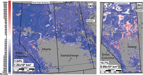
Figure 12. (a) Predicted lake ecosystem critical load exceedances with respect to S_dep. GEM-MACH S_dep scaled using precipitation deposition observations and NEG-ECP (2001) methodology (eq ha⁻¹ yr⁻¹). (b) Predicted aquatic ecosystem critical load exceedances with respect to S_dep, corrected to match precipitation observations, CLRTAP (2017) methodology (eq ha⁻¹ yr⁻¹). (c) Predicted aquatic ecosystem critical load exceedances with respect to S_dep +N_dep, corrected to match precipitation observations (eq ha⁻¹ yr⁻¹) (Makar et al. 2018).

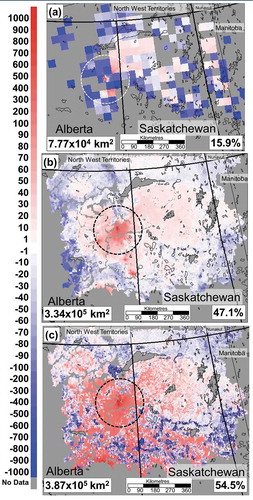
Two different approaches, the simplified NEG-ECP (2001) protocol and the CLRTAP (2017) approach (see “Examples of air pollution–related indicators”), were considered in the determination of critical loads. The estimated terrestrial critical load exceedances (NEG-ECP protocol) cover an area of 1.20 × 10⁴ km². In contrast, the total area estimated to be in exceedance using the CLRTAP (2017) critical loads is more than 5 times higher, 6.99 × 10⁴ km², encompassing about 16% of the region for which data were available within the Province of Alberta. These latter critical load exceedance values include data on province-specific vegetation and soil updates and the use of a more rigorous protocol (see “Examples of air pollution–related indicators”). The inclusion of the observation-corrected base cation deposition estimates derived from the aircraft measurements led to estimates of predictions of more neutralization in the vicinity of the oil sands (circled regions in Figures 11 and 12) relative to initial model estimates (Makar et al. 2018). This is hypothesized to better reflect the dust emissions from the oil sands activities (Makar et al. 2018). However, although this enhanced base cation deposition, which may be interpreted as protective for acidification, it may occur simultaneously with dust deposition of toxics (i.e., PACs and metals), which can also originate from area sources associated with OS development.

Assessment of the current knowledge on PACs

Given the snowpack and lake sediment observations (Kelly et al. 2009; Willis et al. 2018), their known and/or potential toxicity and presence in air, water, and the biota, an integrated program was undertaken for PACs. Monitoring conducted within the ECCC Water Component of JOSM indicated that the amount of PACs and other toxics (e.g., naphthenic acid, metals) seeping from tailings ponds into the watershed is small relative to other sources (Bickerton et al. 2018), suggesting the need to focus on atmospheric pathways between the OS industry and the surrounding environment. Harner et al. (2018) assessed the current knowledge on PACs (before ~2017) in regard to their emissions and transformation, concentrations in air, wet and dry deposition, and insights from source attribution and modeling studies. Three main categories of PACs have been the focus of monitoring in the OS region: polycyclic aromatic hydrocarbons (PAHs), alkylated PAHs (alk-PAHs), and dibenzothiophenes (DBTs and alk-DBTs). These are defined in Section S3.2 of the supplemental material.

Due to the complexity of the transport, transformation, and deposition processes (e.g., particle deposition, deposition with snow, rain, etc.) and lack of knowledge, a comprehensive model to assess local to regional transport of PACs and their by-products and to predict their net influence on ecological systems, as has been done for acidifying pollutants, is not available for the OS region. However, simplified modeling approaches have been applied in the OS region to gain insight into emissions of PACs (Parajulee and Wania 2014; Qiu et al. 2018). These indicate that fugitive emissions of PAHs and alk-PAHs represent the major source to the atmosphere. These include resuspended dust from mine faces, unpaved roads, and petroleum coke storage piles, as well as volatilization from tailings ponds (Figure 13).

Figure 13. (a) Emission sources to air for PAHs in the oil sands region derived from the JOSM emission database (Qiu et al. 2018). (b) Inset map of western Canada showing the Athabasca oil sands region. (c) Zoomed-in map of emissions over the surface-mineable area. Line sources include transportation emissions. Area sources include tailings pond, mine face, mine fleet, community heating, airport, and traffic emissions. Note: oil sands region boundaries are based on 2009 data (Harner et al. 2018).

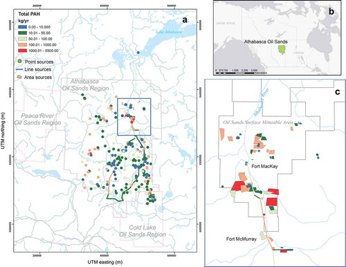
Schuster et al. (2019) documented the long-term concentrations of the three PAC classes across 15 sites in the OS region covering the period 2010–2016. These passive data serve as a key baseline for assessing the impact of future and expanded mining projects in the region on ambient levels of PACs. They have helped evaluate the contribution of forest fire combustion emissions to the PAH levels in air as well as the contribution from revolatilization (during forest fires) of ambient PAHs, which were previously taken up by forests (Rauert, Kananathalingham, and Harner 2017). Forest fire emissions currently play an important role in the PAC levels in the region, one that could increase due to climate change. However, beyond the parent PAHs, there is a lack of information on wood combustion emission factors for alk-PAHs and the DBTs, complicating assessment of the contribution from the OS industry to their levels in water, sediment, and biological compartments (Schuster et al. 2019).

Although forest fires are important, the spatial patterns in PACs observed in the passive sampling network (sites shown Figure S3.10) demonstrate that PACs in air are largely attributed to OS production operations, although levels in different mining-type regions have not been assessed (i.e., PACs arising from in situ versus open-pit mining extraction). The alk-PAHs are the dominant group in the air, and they are attributed to petrogenic sources (i.e., geological sources as opposed to combustion or pyrogenic sources). Observations have shown that other PAC classes, such as DBTs, quinones, transformation products (e.g., nitro- and oxy-PAHs), and a wide range of other PACs (e.g., heterocyclic aromatics), also contribute to the PAC levels in air (Wnorowski 2017).

Consistent with the spatial pattern in air concentrations (Schuster et al. 2019), deposition occurs on a gradient, with higher deposition near oil sands production activity. Spatial patterns of PAC deposition have been explored using a variety of methods, including snow (Manzano et al. 2016), bulk deposition collectors (Bari, Kindzierski, and Cho 2014), lichen (Graney et al. 2017; Landis et al. 2019), moss sampling (Zhang et al. 2016), and a passive dry deposition sampler (Jariyasopit et al. 2018). However, quantitative linkage between concentrations in air and/or precipitation and the levels in these different forms of collection media is difficult to assess (Zhang et al. 2016). Precipitation samples using wet-only collectors have also been deployed in the OS region (Muir et al. 2012). Three “near-field” sites have been operated with monthly collection since 2010. The highest loadings or atmospheric wet deposition fluxes (µg m⁻²) of PACs were observed in the winter months (January–March) in 2011 and 2012 at the two sites closest to the OS operations, whereas loadings at the third site, although only ~10 km north of SML, were 4- to 6-fold lower in winter, but similar from May to October 2012. PAHs (17 unsubstituted) in precipitation at these two close sites were lower than the total annual winter snow fluxes observed at the sites on the Athabasca River, which were within 5 km of these locations (next paragraph). This is likely due to contributions from other sources, such as petcoke and haul-road dust, in the snow relative to the wet-only samplers.

Multiyear JOSM snowpack observations based upon a systematic sampling strategy affirm the pattern shown by Kelly et al. (2009) and also extend the data to greater distances and show that there is considerable year-to-year variability in the magnitude and location of the highest deposition amounts (Manzano et al. 2016; Figure S3.11). Figure 14 shows that there is a rapid drop-off in PAC deposition (accumulated in snow) with distance from a reference site close to the surface mining (AR6 in Kelly et al. (2009)). Beyond 10 km, the deposition appears to be uniform and the shape of the pattern (Figure S3.11) implies that there may be limited directional dependence on deposition amount. However, a more detailed analysis of the decrease in deposition with direction using a Lagrangian trajectory model suggested that regional wind patterns and the intensity of PAC emissions play a role (Cho et al. 2014). Although dependent upon sampling design, Figure 15 suggests that PACs could be spreading further toward the north and south compared with the east and west (Cho et al. 2014). Although the greater spread to the north would be in the direction of the PAD, all measurements of PACs that far north (150–200 km) find that PAC loadings in the PAD are in the same range as found at remote sites in western U.S. national parks (Landers et al. 2010).

Figure 14. Winter 2011, 2012, 2013 and 2014 snowpack total PAC loadings (mg/m²) versus distance (0–25 km) from site AR6, located on the Athabasca River near the Suncor and Syncrude upgraders and roughly in the centre of the major oil sands industrial area (Manzano et al. 2016).

Figure 15. Total mass of the sum of PAHs deposited with distance from the oil sands operations. Case 1 (dotted line) uses the data from only the north and south transect sites, case 2 (dashed line) uses data from only the west and east transect sites, and case 3 (solid line) used data from all transect sites (Cho et al. 2014; Harner et al. 2018).

The long-term temporal trends of PAC deposition first shown for lakes relatively close to the more-active surface mining areas (Figure 3) have now been studied among a larger number of lakes, including those farther away such as in the PAD (Muir et al. 2018). Results from peat cores (Zhang et al. 2016) are also available and largely confirm the temporal and spatial patterns seen from the lake sediments: increases in alk-PAHs, DBTs, and alk-DBTs correspond to the period of OS development and expansion.

Harner et al. (2018) highlighted results of isotopic analysis (Bosch et al. 2015) of sediment cores from a small lake in the PAD (Jautzy et al. 2015). In that work, combined use of ¹³C, ²H, and ¹⁴C provided evidence of the contribution of petcoke from the OS to the phenanthrene in lake sediments in the PAD, thus providing an example of the promise of such approaches for source attribution. Petcoke has been of interest given its open storage at the facilities with on-site upgrading and the toxics it contains. Petcoke has been identified in snow (Zhang et al. 2016), passive air samplers (Jariyasopit et al. 2018), moss (Zhang et al. 2016), and lichen (Landis et al. 2019). Quantitative estimates of petcoke’s and other sources’ contributions to PAHs in moss using chemical mass balance (CMB) have been shown to be feasible (Zhang et al. 2016). Zhang et al. (2016) found that closer to the open piles of coke, the median amount of the PAHs in moss attributable to (delayed) petcoke was 29%, whereas farther away the median dropped to 9%. Among the moss samples examined, the average petcoke contribution was 26%. Emissions from upgrading were estimated to be of similar importance, with an average contribution of 22%. In contrast, there was little evidence that PACs directly from resuspended bitumen was migrating to the locations of moss collection. Although there are ongoing uncertainties associated with source apportionment, as more profiles across a larger range of PACs become available and understanding improves of how profiles change in the atmosphere and/or after deposition, better constraints on the solutions can be expected. Section S3.2.1 of the supplemental material provides a brief overview of some of the other receptor modeling or source apportionment work relevant to the OS region.

Potential impacts of air pollutant deposition on water quality and aquatic effects

The Water Component of JOSM conducted by ECCC focused on seven priority themes related to water quality and quantity, modeling, and benthic and fish health within the LAR and receiving water bodies (Bickerton et al. 2018; Chambers et al. 2018; Culp et al. 2018b; Droppo et al. 2018a; Glozier et al. 2018; Kirk et al. 2018; McMaster et al. 2018). These main activities are summarized in the supplemental material (see Sections S4.1, S4.2, S4.3), and this section focuses on results related to atmospheric deposition and understanding the fate and impacts of this deposition on water quality and aquatic species.

Atmospheric deposition patterns of mercury and trace metals

Paleosediment cores from a wide spatial distribution of lakes across the oil sands region indicated that PACs and inorganic contaminants (e.g., vanadium) increased since the OS development began (1960s), with impacts most pronounced in lakes <50 km from the major development area (Kirk et al. 2018). In addition to PACs (Figure S3.11), mercury and a suite of trace metals were measured in the late winter snow samples collected at a large number of locations (Kirk et al. 2014). Consistent with previous work (Kelly et al. 2010, 2009), the peak deposition was observed close to the most active surface mining and upgrading areas and dropped off with distance. Figure 16 shows the pattern for total and methyl mercury (THg, MeHg) reported by Kirk et al. (2014). Seventy to eighty percent of species were bound to particulates >0.45 μm in size, which helps explain the higher loadings closer to the sources given gravitational settling. Comparing the values between the maps shows that the percent MeHg was quite low (average 2.5 ± 1.7% in 2012).

Figure 16. Deposition of THg (left) and MeHg (right) to the Athabasca oil sands region in winter 2012. Contours of THg and MeHg loads (ng m^-2) were produced through Kriging of the measured values shown by the colored circles (Kirk et al. 2014).

Deposition at the most distant sites studied, which were in the PAD, were found to be consistent with the baseline deposition approximated as the amount at the far reaches of the ~20,000 km² zone measured and mapped in Figure 16. Spatial patterns in V, Zn, and Ni, which are emitted from OS operations, were highly correlated with the THg and MeHg concentrations (r = 0.73−0.86, P < 0.01), suggesting that mercury, including MeHg, has similar source locations. Furthermore, the strength of the correlations imply that MeHg is emitted directly from some OS activities. An alternate explanation for the high correlation between THg and MeHg could be that the latter is formed from THg in the snowpack. However, Willis et al. (2018) found that this in situ production is unlikely to be an important net source of MeHg in the snowpack.

Crustal elements, and total suspended solids, deposition closely followed the mercury spatial pattern, whereas spatial correlations with dissolved organic carbon (DOC) and sulfate were lower, indicating different sources or transport pathways for these species. By integrating the total amount of THg deposited within 50 km of a central point in Figure 16 (referred to as AR6 in Kelly et al. [2009]), Kirk et al. (2014) estimated that a total of <1.9 and 0.05 kg of THg and MeHg, respectively, were deposited to the landscape during the <4-month period of snow accumulation (i.e., between the first major snowfall and sampling in the spring). This is less than the 17 kg of THg they estimated was emitted during that time period by assuming that annual atmospheric emissions in NPRI did not vary greatly from month to month. Thus, the results from the snowpack are much less than the emissions reported, suggesting that the emissions may be overestimated in the NPRI or a large percentage of what is emitted is not captured by the snow sampling or is transported further than 50 km or that a portion of the mercury deposited within 50 km is lost, post deposition, and so is not detected in the snow. THg and MeHg can undergo postdepositional processing in snowpacks, likely by photoreduction and photo-demethylation. However, understanding of the processes controlling Hg in the surrounding environment remains poor, which was also demonstrated from observations of the behavior of mercury observed in lichen (Blum et al. 2012). In contrast, through the same estimation procedure, Kirk et al. (2014) found that the amounts of V and Ni in the snowpack within 50 km were about double the reported emissions, whereas the amount of Zn deposited was more than 8 times the amount reported to NPRI.

There is little understanding of how the contaminants deposited on land, as indicated by the snow samples, may be transformed biogeochemically as they move through the sediment continuum from hill slope to aquatic depositional areas (Droppo et al. 2018b). There are also multiple ecological processes controlling rates of contaminant bioaccumulation and biomagnification through food webs during and after this transport into the tributaries and the LAR. Comparisons of PAH assemblages in snow and spring melt surface waters reveal considerable differences (Birks et al. 2017).

Toxicological assessment of the potential impact of contaminants deposited to the snowpack

Toxicological assessments have focused on laboratory studies using fathead minnow larvae. These chronic exposure studies (i.e., ≥3 weeks), using melted snow from sites near the mines and industrial stacks, demonstrated that there is decreased larval fish survival (McMaster et al. 2018; Parrott et al. 2018). However, exposure to freshet water (i.e., spring meltwater) did not impact survival, suggesting that the dilution occurring in the region is sufficient to limit impacts to fish. Species such as walleye and white sucker have embryonic developmental periods of 18–20 days and so may be more sensitive than fathead minnow to the contaminants in snow and spring meltwaters (Parrott et al. 2018).

The apparent elimination of toxicity from snow melt to spring run off in the tributaries, likely due to dilution of the contaminant exposure, was further explored by comparing the sum of PAHs + alk-PAHs in snow and spring meltwater. Parrott et al. (2018) reported that the total concentration of PAHs + alk-PAHs in spring meltwater collected near the largest amount of deposition (see Figure S3.11) was about 50 ng L⁻¹, whereas the concentrations in snow near this location (AR6) ranged from 23,815 to 273,140 ng L⁻¹. Evaluation of which of the deposited contaminants in the snow were most responsible for the fish toxicity observed from the melted snow suggested that PACs were the likely cause (Lee et al. 2015; Parrott et al. 2018). Metals were not deemed to be responsible for the observed effects, given their snow concentrations relative to water guidelines; only 13 of the 45 metals measured have a water quality guideline (CCME, Canada 1999). Similarly, effects were also not suspected to be due to naphthenic acids in snow close to industrial operations (Parrott et al. 2018). However, it is possible that other PACs containing N and S heteroatoms, which were also characterized by Manzano et al. (2016), could be associated with the observed effects (Parrott et al. 2018).

Comparisons of the toxicity of snow samples using the laboratory techniques revealed that there were differences between years, with 2012 snow being the most toxic and having the highest PAHs and 2013 being the least toxic. These differences were consistent with PAC loading estimates in snow samples collected over the same period (Manzano et al. 2016). Differences in toxicity or potency over shorter timescales, such as at different times in spring melt, could also occur in the OS region. However, Parrot et al. (2018) did not collect multiple spring meltwater samples over time (within a year) to assess potential differences in contaminant concentrations and effects on fish. The toxicity of snow varied among sampling locations. However, the effects were not necessarily linked to the quantity of alk-PAHs (Parrott et al. 2018). The reasons for this behavior could be due to the form of the PACs in the snow, as it appeared that the less potent, but higher-alk-PAH snow contained particulate dust from the piles of petcoke nearby. This lower potency could be indicative that PACs associated with petcoke particles may be largely unavailable to larval fish. In contrast, snow from a different location in the OS region that was less impacted by petcoke dust (evidenced by particles that were brown and finer-grained compared with the petcoke-impacted site) had considerable potency, but lower alk-PAH concentrations, implying that in these snow samples the particle-bound contaminants may have been more bioavailable to the fish.

Monitoring water quality in the Athabasca River tributaries

Tributary monitoring occurred on 15 tributaries (10 on the west side and 5 on the east side of the Athabasca River), in addition to the Clearwater River and several of its tributaries, from April 2012 to March 2015. Sampling locations are shown in Chambers et al. (2018) (see Figure 1, and Section S4.4.1 of the supplemental material). The highest concentrations of the target parameters were observed during snowmelt periods or rain events, suggesting a link to atmospheric deposition, although enhanced erosion was also likely involved. This uncertainty masks our knowledge of the relative contributions of atmospheric particulate material within the rivers versus that derived from natural aquatic and terrestrial erosion. There was a slight variation to the general pattern of snowmelt or rain event peaks for MeHg, which showed increasing concentrations with increasing flow during spring. However, the greatest concentration of MeHg occurred during the mid- to late-summer months when MeHg production is principally controlled by microbial pathways. The majority of inorganic and organic contaminants did not exceed the Guidelines for the Protection of Aquatic Life (CCME, Canada 1999). Where exceedances did occur, they were mostly associated with the spring freshet and large rain events when suspended sediment and loadings are typically high. Only pyrene from the PACs showed occasional exceedances for established guidelines (Chambers et al. 2018).

Analysis of historical tributary water quality data (1972–2010) showed no discernible change in concentrations and loads of total V, dissolved Se (diss Se), and dissolved As (diss As) prior to OS development when sampled above versus below the McMurray formation (Alexander and Chambers 2016). These observations were thus used to represent reference chemical conditions (i.e., water chemistry associated with predevelopment conditions). Following increases in OS development, concentrations and loads were often greater downstream of development compared with measurements from (unimpacted) reference sites (Figure 17). This historical analysis is suggestive of a possible influence of OS development on total V, diss Se, and diss As concentrations and loads. In addition, concentrations tended to be highest during the land-clearing phase of development (Alexander and Chambers 2016; Chambers et al. 2018).

Figure 17. Mean annual (2012–2014) concentrations of dissolved arsenic (diss As), dissolved selenium (diss Se), and total vanadium (total V) at upstream (U) and downstream (D) sites on three Athabasca River tributaries (Ells, Muskeg, Steepbank). Significant differences (P < 0.05) are identified (*) between upstream and downstream sites on the same river (Ells, Muskeg, or Steepbank) or the three rivers overall (Chambers et al. 2018).

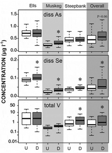
A case study, focusing on the Muskeg River (1972–2009 data), provided insight into the impacts of development and land disturbance (Alexander and Chambers 2016) on tributary water quality. Data from sites on the river were grouped into three categories: upstream of development (MU7); just downstream of development (MU4); and downstream of development (MU1) as well as downstream of incisement of the McMurray Formation (Figure 18). Reference conditions were estimated by pooling concentrations from all upstream sites and the downstream sites sampled prior to development (Figure 18; Alexander and Chambers 2016). Concentrations of diss As, diss Se, and total V were greatest during the early stage of mine development at MU4, the site situated closest to active development (13–35% greater than reference). Kelly et al. (2010) also observed that concentrations of metals such as cadmium and zinc were correlated with the extent of land disturbance in the watershed. Concentrations of diss Se were also elevated during the subsequent development phase at the furthest downstream site (21% greater than reference). During the early phase of mine development, diss As, diss Se, and total V loads were 34–126% greater immediately downstream of development and 47–148% greater at the furthest downstream site compared with reference loads (Figure 18) (Alexander and Chambers 2016; Chambers et al. 2018).

Figure 18. Muskeg River watershed showing: (a) the three aggregate study sites: MU7, situated up stream of development; MU4, situated just downstream of development and; MU1 (near the river mouth), situated downstream of development as well as incisement of the McMurray formation; (b) concentrations of dissolved As, dissolved Se and total V at the upstream site (MU7) and two downstream sites sampled prior to development; (c) average daily loads (kb/day) of dissolved As, dissolved Se and total V at the downstream site (MU1), with the stage of mining operations identified for the period of record; (d) annual loads (2012-14) only) of dissolved As, dissolved Se and total V at upstream (MU7) and downstream (MU1) sites. (Chambers et al., 2018).

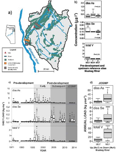
Analysis of more recent data for the Muskeg River (i.e., data collected during JOSM) found that annual loads of diss As, diss Se, and total V were >200% greater downstream compared with upstream of development (Figure 18). However, differences in upstream versus downstream loads varied seasonally: differences were greatest during snowmelt for diss As (12.99 ± 8.15 vs. 3.00 ± 1.46kg year⁻¹ for downstream versus upstream, respectively, P = 0.03), but greatest during the open-water period for diss Se and total V (both >4× greater, P = 0.04 and P < 0.01 for diss Se and total V, respectively).

Tributary water composition has also been studied in the context of acidity given that OS operations emit potentially acidifying pollutants to the air and large tracks of northeastern Alberta are acid sensitive. Analyses assessing 83 snowmelt events on five Athabasca River tributaries between 1989 and 2014 found that 32 of the snow melts studied (39%) exhibited acidification (pH < 7) episodes (Alexander, Chambers, and Jeffries 2017). The 2012–2014 data showed that snowmelt concentrations of 11 priority pollutants and Al were always higher during low pH episodes (Alexander, Chambers, and Jeffries 2017). This finding is consistent with reports from Dickson (Dickson 1978) and Lawrence (Lawrence 2002) that acidification episodes are often associated with high stream flows and can cause mobilization and transport of contaminants such as metals from the land base to adjacent water courses.

Monitoring water quality in the Athabasca River and the PAD

Similar to the tributaries, guideline exceedances were few and generally occurred during spring freshet when suspended solids and contaminant loads are high. Section S4.4.2 of the supplemental material discusses the LAR monitoring implemented in JOSM. Total iron, aluminum, and copper had very high exceedances, which is not uncommon for earth elements. Overall, dissolved parameters often showed an inverse relationship to the hydrograph, whereas those contaminants associated with the particulate phase increased with flow. For the parameters assessed to date, which included total phosphate (TP), dissolved organic carbon (DOC), THg, MeHg, and metals (As, Se, V, and B), there was an increase in concentration from above Fort McMurray to below, but thereafter these parameters exhibited relatively constant concentrations to the PAD. This increase is suspected to be due to the sewage treatment plant and influence from the Clearwater River (Glozier et al. 2018). Concentration ranges for both THg and MeHg overlapped throughout the entire study area, and longitudinal patterns were similar for both of these forms of mercury.

Variations in mercury levels in the PAD tributaries that were sampled were complex, and the reasons are not well understood. This highlights the challenge associated with studying water quality in the PAD and linking observations to possible sources such as the OS development, either from transport down the LAR or in the atmosphere. For example, samples in downstream reaches of the LAR, Peace River, and Slave River, as well as the Birch and McIvor rivers, frequently exceeded the CCME guideline for THg for the protection of aquatic life (CCME, Canada 2003). Mean, median and ranges of THg and MeHg concentrations were greatest in the two westernmost tributaries, the Birch and McIvor rivers. Also, as with major ions and nutrients, the total and dissolved metals measured in the tributaries of the PAD showed a large range and variability and distinct patterns among sites depending on the parameter. However, understanding the reasons for this large “within-PAD” variability will need to improve before the impact of “external inputs” (e.g., atmospheric deposition from the OS, flow down the AR) can be quantified.

In addition to examining PAC concentrations and variations in space and time with grab samples along the LAR, semipermeable membrane devices (SPMDs) were deployed to passively sample multiple species, particularly PACs, from the river water. Yang et al. (2011) identified a typical PAC profile for bitumen from the OS region. Bituminous samples are dominated by alkylated naphthalenes, fluorenes, phenantherenes/anthracenes, fluoranthenes/pyrenes, and dibenzothiophenes. When Yang et al. (2011) combined SPMD data from the LAR and rivers of the PAD from 2013 to 2015, the typical bitumen PAC profile was evident. However, this profile was only evident in SPMD samples collected from sites within and downstream of the bituminous area of the Athabasca main stem. Typical of bitumen within the OS region, concentrations of alk-PAHs in the SPMD samples obtained within and downstream of the bituminous area were higher than those of unsubstituted, parent compounds, which were dominated by naphthalenes, fluorenes, phenanthrenes/anthracenes, fluoranthenes/pyrenes, and dibenzothiophenes. There were also measurable concentrations of PACs with five and six benzenoid rings (e.g., benzofluoranthenes, benzopyrenes, dibenz[a,h]anthracene, perylene, benzo[g,h,i]perylene, and indeno[1,2,3-c,d]pyrene), which are among the compounds identified as Priority Pollutants (PPs) by the EPA (2019b) and recognized as carcinogenic by the CCME. Collectively, the SPMD results suggest that natural erosion of bitumen plays a role in the LAR water chemistry, but atmospheric deposition is also contributor.

Most PACs measured using the SPMDs exhibited similar spatial and temporal concentration changes (Glozier et al. 2018). This is illustrated in Figure 19 by the pattern of C₄-phenanthrenes/anthracenes, which had the highest average concentrations (Glozier et al. 2018); concentrations were lowest outside the OS area in the Peace and Slave rivers, and in two PAD wetlands. Higher concentrations were recorded at sites located within the bituminous watershed of the AR, notably immediately downstream of the Clearwater River and near the Muskeg River. Concentrations within the LAR downstream of the bituminous area were slightly lower and retained the Athabasca oil sands chemical signature. Tributaries within the PAD (Richardson, Quatre Fourches, and Birch rivers) also contained measurable concentrations of PACs.

Figure 19. Concentration of C₄-phenanthrenes/anthracenes (ng/L) from 2013 to 2015 at seven Athabasca River main stem sites (M0 through M9), tributaries, and wetlands in the Peace-Athabasca Delta (PAD) and the Peace and Slave Rivers (Glozier et al. 2018).

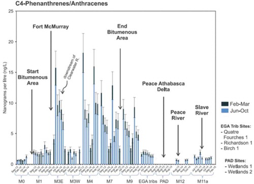
Seasonally, concentrations of PACs were notably lower during the under-ice period than during the open-water season (Figure 19). This pattern in PAC concentrations differed for the more volatile PACs and some of the bitumen-specific compounds. Volatile PACs were nearly absent upstream of the OS, peaked in the OS mining area, and decreased in concentration with distance downstream of the OS mining area (i.e., Slave and Peace rivers, PAD tributaries). This suggests evaporation into the air as one mechanism for the downstream decrease in the concentrations of these species. OS dibenzothiophenes were greatly reduced in concentration far downstream of the OS mining area (i.e., in the Slave River) compared with further upstream, likely due to the dilutive effect of the Peace River upon confluence with the LAR. Other PACs, such as indeno[1,2,3-c,d]pyrene, were also absent from samples collected upstream of the OS region and more remote areas such as the PAD. Although indeno[1,2,3-c,d]pyrene has been associated by other studies with oil production and refinery effluent discharges (Harman, Farmen, and Tollefsen 2010; Parrott et al. 1999), the monitoring in the LAR suggests that Fort McMurray may be contributing. For example, on the east side of the river, it was present at its highest concentrations immediately downstream of the Clearwater River (and Fort McMurray) (Glozier et al. 2018).

Methods developed for the investigation of the biological/ecological condition of aquatic ecosystems

To evaluate the efficacy of monitoring designs to answer bioassessment questions that can potentially detect impacts from the OS development, studies of benthos, caged mussels, and fish in the LAR main stem, tributaries, deltaic and extended geographic ecosystems were undertaken (Culp et al. 2018b). In the LAR main stem, the benthic assemblages largely exhibited good ecological condition, with intolerant taxa found in large abundances at all sampling sites. However, Culp et al. (2018b) demonstrated some shifts in diversity depending upon location. This suggests that studies of benthic assemblages can be sensitive indicators of impact, but at present the main shift observed is difficult to attribute to the OS development. The middle reaches of their study area exposed to municipal sewage effluent from Fort McMurray (includes nutrients) and OS development showed increased relative abundance of tolerant taxa (Culp et al. 2018b). However, at sites considerably downstream of the development, the community distribution shifted back toward reference conditions upstream of the disturbance (Culp et al. 2018b). Although the observed difference in middle-reach benthic communities was associated with trends of high algal biomass, definitive linkage of environmental drivers to this ecological change will require direct examination of associations between the longitudinal benthic pattern and key supporting variables (e.g., nutrients, PACs, V) through additional field experiments.

Similar to the LAR main stem, benthic assemblages in the tributaries generally exhibited good ecological condition, with high abundance of intolerant Ephemeroptera (mayfly), Plecoptera (stonefly) and Trichoptera (caddisfly) (EPT) taxa among the sites. Biological conditions at reference sites located outside of the OS region but within the natural deposit were found to be similar (Culp et al. 2018b). However, benthic assemblages in areas with an increased OS impact were divergent from these reference sites. Further investigation is required to determine whether there is a causal relationship between exposure to environmental stressors associated with OS development and this altered assemblage composition as the biological change was confounded between natural processes (e.g., erosion) and development.

The PAD wetland monitoring sites represented two potential, distinct exposure pathways: (1) surface flow and associated sediment deposition from the LAR and (2) atmospheric transport and deposition of emissions in the form of snow, rain, and/or dust particles. Despite potential contributions from these exposure routes, PAD macroinvertebrate assemblages appeared to be in a healthy state, exhibiting high biodiversity, as well as strong seasonal and spatial variability of richness and composition (Culp et al. 2018b). Thus, to date, there is no evidence of cumulative effects (on benthos species) in these deltaic ecosystems arising from OS activities.

Mussels exposed to middle-reach waters were less able to cope with stress tests and, compared with reference sites, mussel condition was lower at sites downstream of the OS development area (Pilote et al. 2018). These longitudinal patterns may indicate mild environmental stress related to the combined effects of nutrient (sewage treatment effluent) and contaminant stressor (i.e., natural or emitted OS contaminants) exposure.

Monitoring of fish health in OS region was built upon the methods developed for Canada’s Environmental Effects Monitoring program (e.g., McMaster, Hewitt, and Parrott 2006). To assess the ability of these methods to identify potential impacts sampling locations encompassed reference sites inside and outside the OS deposit that were both upstream as well as downstream of development. White suckers were used to assess changes because in previous work (Arciszewski et al. 2017b) they were found to be sensitive indicators of fish health in relation to sampling downstream and within the OS deposit. However, similar to the main stem benthic results, the pattern observed thus far is indicative of nutrient enrichment, as white sucker were older, longer, and heavier than reference fish thus exhibiting increased condition and increased levels of internal fat stores. White suckers within the deposit also exhibited exposure to PACs, as their livers had significantly increased enzyme activity (i.e., induced biomolecular changes; Arciszewski et al. 2017b).

Fish health research in the tributaries conducted by the JOSM Water Component developed health baselines for sentinel species, primarily the slimy sculpin, and used this information to determine the potential for OS development to affect overall fish health (Parrott et al. 2018). Slimy sculpin were found to be sensitive biological indicators, as shown by consistent changes in fish health between reference and exposure sites within the OS deposit. The recorded end point changes included increases in liver size with corresponding biomolecular changes (i.e., induction of ethoxyresorufin-O-deethylase [EROD] activity) for fish collected at exposure sites as well as reductions in energy invested in reproductive development, as represented by lower gonadal development. These downstream responses are indicative of exposure to inducing compounds, as EROD activity followed a similar pattern to PAC body burden, the latter of which is shown in Figure 20. Moreover, assessment of sediment toxicity suggested that sediments were the source of the elevated PACs in the water column (McMaster et al. 2018). Controlled exposures of fathead minnows to natural oil sands sediment from two river sites (Steepbank River and Ells River lower sites) demonstrated decreased embryolarval fish survival (Parrott et al. 2018). However, continuous exposure of resident fish to sediment within the oil sands deposit appears to be required for the increased expression of EROD activity at these sites (McMaster et al. 2018). Similar to the tributaries, sculpin in the LAR within the OS deposit area also appeared to be exposed to compounds that induce biomolecular changes (inducing compounds). Furthermore, there is evidence that exposure to these compounds is higher downstream of development (McMaster et al. 2018).

Figure 20. Polycyclic aromatic compounds (PACs) levels in female slimy sculpin collected from the Steepbank River during the fall of 2012–2013. Sites represent the Steepbank lower site (lower and RAMP lower: same site), Steepbank mid site (MC Mid), Steepbank upper site (MC Upper), and a site further upstream (RAMP Upper). Values represent the mean ± SE. Parent PAHs: pink; alkylated PAHs: green; total PAHs: blue. (Reproduced from Culp et al. 2018b.)

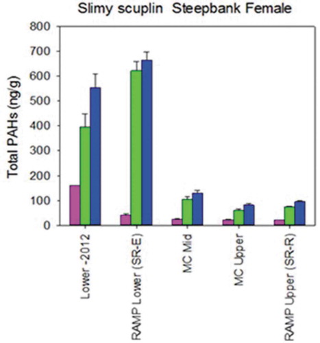
Establishing a methodology for causal assessment of ecological effects

Attribution to the OS development activities and related atmospheric deposition remains uncertain given other stressors (e.g., Fort McMurray sewage treatment plant releases to the AR) and inputs from natural bitumen erosion. The impact of human activities in aquatic ecosystems is most often the result of multiple stressors associated with different sources of stressors (Norton, Cormier, and Suter 2015). Because of this, it is challenging to link ecological effects to individual stressors or the combined, interactive effects of multiple stressor threats. An effective approach for analyzing a large body of evidence of stressor effects on ecological components of aquatic ecosystems is the use of weight-of-evidence approaches such as the ecological casual assessment method proposed by Norton, Cormier, and Suter (2015). This approach, which can assess data from different sources, such as of pollutants from natural erosive processes or atmospheric deposition, is being implemented to evaluate its utility to collectively assess their relative potential to cause ecological effects in the context of the OS (Culp et al. 2018a). Results are suggestive that this weight-of-evidence approach can enable the linkage of ecological effects and candidate causes and forward plausible support as to the importance of these pathways (Culp et al. 2018a).

Causal pathways suggest that the observed LAR ecological trends were associated mostly with nutrient enrichment from treated municipal sewage effluent from Fort McMurray. However, the combined contaminant exposure from sewage effluent, industrial operations (atmospheric deposition), and natural exposure to bitumen may also be contributing to these ecological trends (Culp et al. 2018a).

Potential impacts of air pollutant concentrations and deposition on wildlife

The Wildlife Contaminants and Toxicology Component’s main objective was to assess the health of wildlife species that are potentially exposed to OS-generated contaminants. In terms of direct wildlife impacts, the key chemicals of concern were PACs, Hg and MeHg, trace metals, and naphthenic acids. Each has the potential to cause toxicity, and some can bioaccumulate and biomagnify in biota and may persist in the environment (Achten and Andersson 2015; Clarkson 1993; Clemente and Fedorak 2005). A sentinel species (see Section S5.3 of the supplemental material) approach was adopted to gain a better understanding of exposure routes, impacts, and the biological mechanisms involved, potentially enabling development of a long-term wildlife contaminant and toxicology monitoring program. As such, in-depth monitoring and research projects were carried out with multiple species to assess the presence and effects of contaminants in plant communities, in terrestrial and wetland species, and in downstream receiving environments.

The main sentinel species used in the Wildlife Contaminants and Toxicology Component projects are listed in Table 1; ecological surveys and sampling strategies varied among the species listed. For amphibians, migratory birds, and plant communities, and semiaquatic furbearer species, all of which stay within localized areas during the key periods of interest, exposed (i.e., near to the OS operations) and control or baseline locations were studied and compared. Multiple representative sites for each of these conditions were identified, and sampling was largely carried out in 2012–2014, with some continuing to 2018. For colonial waterbirds, the PAD was of interest given the potential for accumulation of contaminants of concern (COCs) from atmospheric deposition and transport down the LAR.

Table 1. JOSM Wildlife Contaminants and Toxicology Component sentinel species.

Species group	Sentinel species	Contaminants
Mammals^#	Muskrat (Ondatra zibethicus)	Heavy metals, PACs, trace metals
	Beaver (Castor canadensis)
	American marten (Martes americana)
	Mink (Neovison vison)
	River otter (Lontra canadensis)
	Fisher (Martes pennanti)
Colonial waterbirds	Caspian tern (Hydroprogne caspia)	As, Hg, PACs
	Common tern (Sterna hirundeo)
	Ring-billed gull (Larus delawarensis)
	California gull (Larus californicus) Herring gull (Larus argentatus)
Amphibians	Wood frog (Lithobates sylvaticus)	Hg, PACs
Plant health and community composition	Wetland/upland vegetation communities	Trace metals, PACs
Migratory birds	Tree swallow (Tachycineta bicolor)	PACs

^#See Section S5.5.2 of the supplemental material.

The wildlife species listed in Table 1 were able to provide information on contaminant burdens and spatial and temporal trends of COCs in the region and were used to assess toxicological responses to COC exposure. Thus, these species were used to provide the insight needed for evaluating the health of native species and generate information on overall ecosystem health (Cruz-Martinez and Smits 2012). In addition, studying some of these species provided information related to food safety and food security concerns for local indigenous land-users, and/or were also potentially important species (i.e., valued ecosystem components) as a result of their cultural and traditional values or their importance for local economic livelihood. See Section S5.5.2 of the supplemental material.

Plant health and community composition

Using on-site vegetation surveys (see Section S5.5.3 of the supplemental material) and observations from the corresponding seed bank germinated in the laboratory (from soil samples), it was found that OS sites had greater species richness compared with the east and west reference sites, although this difference was only significant for OS versus east sites. However, overall, diversity was high across the sites, with 290 herbaceous and woody plant species identified in the region, of which over 85% were perennial species (Boutin and Carpenter 2017). The added richness at the OS sites was mainly composed of non-native or introduced species, compared with reference sites that were almost exclusively native perennials.

OS sites also had greater levels of PACs in soil and vegetation (above- and belowground plant parts) compared with the reference sites. Although the relative proportion of alk-PAHs and parent PAHs were not significantly different among sites (soil and vegetation), with alk-PAHs being more prevalent, there were differences in the distribution among PAC species (soil) among some sites (Boutin and Carpenter 2017). Soil guidelines (Ontario and/or EPA) were exceeded for several of the parent PAHs at some of the OS sites. There was a significant negative correlation between site minimum distance to an upgrading facility and the total concentration of parent PAH compounds and a weaker, nonsignificant correlation with alk-PAHs. Distance to the nearest upgrader facility was also significantly correlated to trace metal concentration for 13 of the 28 metals measured with elevated levels at OS sites (Boutin and Carpenter 2017). There were guideline exceedances for 14 out of 28 metals measured, predominantly at the OS sites (Boutin and Carpenter 2017). Further investigation is required to determine how specific contaminants affect plant species and to understand potential contaminant burdens in the food web.

Amphibians

Boreal wetlands closer to the OS facilities receive spring melt containing significant amounts of atmospheric contaminants that were deposited and accumulated in the snow over winter. As discussed above, the link between these contaminants and their levels in tributaries and the LAR is complex, but local wetlands may be more directly impacted and are thus an important ecosystem to monitor. As the spring melt coincides with the wood frog breeding season, wood frog early life stages may be exposed to potentially high COC levels during early stages of development. In particular, amphibians may be exposed to detrimentally high levels of PACs during embryo development, which is a particularly sensitive point in their life cycle (Mundy et al. 2018). Amphibians have shown to be sensitive indicators of wetland quality during previous studies on wetlands containing OS processed water (Hersikorn, Ciborowski, and Smits 2010; Pollet and Bendell-Young 2000).

Under the Amphibian and Wetland Health program, samples were collected from wetlands close to and more distant from OS industrial facilities to measure concentrations of the COCs in amphibian breeding habitat. Measurements were obtained in wood frog tadpoles, and, in addition, PAC concentrations were measured using semipermeable membrane devices (SPMDs). These SPMDs were deployed at the same wetlands for 5–6 weeks close to the locations of wood frog egg masses. The PAC profiles found in the wood frog tadpoles and the SPMDs were dominated by C₁–C₄ alk-PACs, indicating petrogenic sources (Mundy et al. 2018). Although the total PACs in wood frog tadpole tissue did not differ significantly between wetland sites, SPMDs deployed within a 25 km radius of surface mining activity measured the highest concentrations of PACs, showing a significant exponential relationship between PAC accumulation and distance to OS mining activities (Figure 21), consistent with the snow deposition studies discussed above. The site closest to the OS upgrading facilities, which was along the north-south highway adjacent to SUN and SML, had SPMD PAC levels that were approximately 10-fold and 3-fold higher than the other wetland sites in 2013 and 2014, respectively (Mundy et al. 2018). In the wood frog tadpoles, total PACs were 25% higher at this closest location; however, there were no statistically significant differences among the locations for parent PAHs or the alk-PAHs overall. Mercury and MeHg and trace metals were also measured in wood frogs and their habitat; levels were generally low and did not reveal a spatial pattern in relation to distance to air pollution emission sources, although levels infrequently surpassed the CCME guideline levels for the protection of freshwater aquatic life (CCME, Canada 1999).

Figure 21. (A) ∑PACs detected in SPMDs (ng SPMD⁻¹) deployed in the Athabasca oil sands region (AOSR). Field blank corrected. Bars represent the mean, with error bars representing the standard error of the mean from duplicate (Gateway 2014, Hat-S5) and triplicate SPMD deployments. Wetlands study sites are arranged on the x-axis from nearest to furthest from oil sands upgraders. (B) ∑PACs accumulated in SPMDs (ng SPMD⁻¹) deployed in 2013 and 2014 as a negative exponential relationship with distance from oil sands industrial development (r² = 0.89). PAC values are field blank corrected; error bars represent the standard error of the mean of detected PAC analytes. Note: Gateway wetland was not included in this analysis because it is adjacent to a reclaimed overburden pile. (C) ∑PACs accumulated in SPMDs represented as C_free (pg L⁻¹) deployed in 2013 and 2014 as a negative exponential relationship with distance to upgraders (r² = 0.66). As noted above, Gateway wetland is not included in this analysis (Mundy et al. 2018).

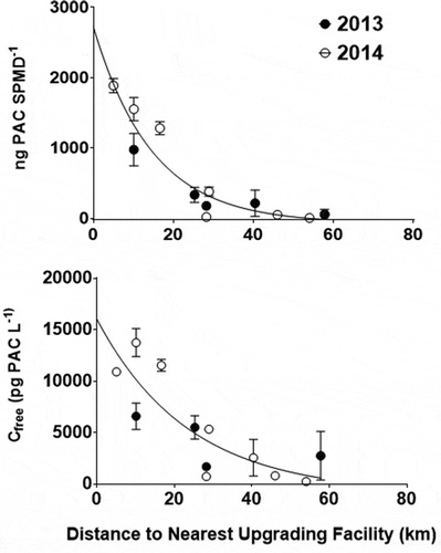
Discrepancies among SPMD accumulation of PACs and invertebrate tissues have been observed in other studies, as described in Mundy et al. (2018)). Thus, laboratory studies were conducted to improve understanding of the wood frog tadpole exposure routes and metabolism of alkyl and parent PACs using sediment collected from the McKay River in the OS region (Bilodeau et al. 2019). The wood frog tadpoles exposed to PAC-laden sediment and water were found to rapidly accumulate and commence elimination of most PACs within 12–24 hr of exposure (Bilodeau et al. 2019) and reach an equilibrium within 12–48 hr. Multiple linear regression analyses showed that PAC concentrations in the sediment were a better predictor of PAC concentrations in the wood frog tadpoles than the water concentration during combined exposure experiments. The wood frog tadpoles accumulated more total alk-PACs than parent PACs, as well as higher concentrations of the alkylated compounds, compared with their respective parent compounds. There was also a clear petrogenic PAC profile observed in the wood frog tadpoles; this closely resembled the profile of the McKay River sediment to which they were exposed (Bilodeau et al. 2019). Overall, both parent and alkyl-substituted PACs had low bioaccumulation potential, with anthracene, fluoranthene, retene, and C₁-benzofluoranthenes/benzopyrenes having the highest potential and only C₄-naphthalenes persisting in wood frog tadpoles after 48 hr of depuration. Thus, the results of the laboratory experiments suggested that the wood frog tadpoles seem to be efficient at metabolizing and eliminating most parent and alkyl-substituted PACs (Bilodeau et al. 2019).

Despite the complicated exposure pathways and bioaccumulation behaviors of PACs in wood frog tadpoles, the results to date suggest that it might be possible to use SPMDs to monitor PACs in natural wetlands in the OS region, and possibly to replace sampling of wood frog tadpoles with SPMD deployment in an effort to replace invasive and lethal animal sampling with the use of passive samplers. However, there is a need for further validation of SPMDs as surrogates for wood frog tadpoles; considerations around water chemistry interactions and PAC uptake by wood frog larvae and tadpole PAC metabolism in relation to SPMD accumulation need to be addressed (Weinhold 2011). Nevertheless, use of SPMDs as passive environmental samplers shows promise for the assessment of the potential exposure of resident wetland species to PACs, and with further investigation this approach might be used to monitor, model, and assess the risk for potential toxicological impacts over space and time.

Migratory birds

In the OS region, PACs can accumulate in sediments and aquatic insects, resulting in a high exposure potential to PACs for nesting tree swallows that primarily consume aquatic insects (Fernie et al. 2018a). In the past, biological responses of tree swallows breeding on reclaimed wetlands in the OS region have been studied (Cruz-Martinez et al. 2015; Gentes et al. 2007; Godwin, Barclay, and Smits 2019; Harms et al. 2010). During JOSM, colonies of nest boxes for breeding tree swallows were established adjacent to water bodies (Figure S5.1) at four study sites in 2012 and 2013 (Fernie et al. 2018a). Two colonies were located in the surface mining area of the Fort McMurray region, within 5 km of active mining, extraction, and processing (OS sites). Two other colonies were established at reference sites, one in 2012 and the other in 2013, more than 100 km from regional OS operations (Fernie et al. 2018a).

At the sites, samples of blood, pectoral muscle, dorsal feathers, and feces were collected from the tree swallow nestlings, along with passive air samples (measurements including SO₂, NO_x, hydrogen sulfide [H₂S], and VOCs) and grab samples of water. Twenty-one analyzed parent PAHs, all 13 alk-PAHs, and 4 of 5 DBTs were found in nestling (muscle and feces), air, and water samples, and for most PACs levels were higher at OS sites compared with reference sites (Figure 22). These data enabled PAC tissue concentrations of tree swallows to be described in relation to concentrations in the air and water. Compared with reference sites, tree swallow nestlings developing near active mining sites located in the OS region accumulated higher concentrations of PACs, and exposure route importance was dependent on the specific compound.

Figure 22. The concentrations of the six major PAHs measured in nestling tree swallows (ng/g wet weight). Concentrations were similar between the reference birds (REF1, REF2), and significantly higher (P ≤ 0.05) in the birds from the oil sands mining–related sites (OS1, OS2) in the Athabasca oil sands region (Fernie et al. 2018a).

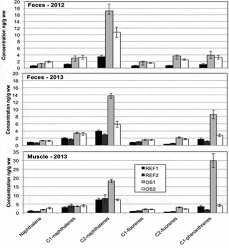
Two main, interrelated outcomes were studied in the tree swallows: thyroid morphology and hormones (Fernie et al. 2019) and reproductive success and developmental changes (Cruz-Martinez et al. 2015; Fernie et al. 2018). As described above, the nestlings were exposed to a combination of stressors. Thus, although it is difficult to tease out cause of the effects observed, these studies were able to use statistical models to identify which of the measured stressors contributed to the changes observed in the tree swallows. However, results suggest that the greatest influences on avian thyroid function in the OS region, especially the thyroid gland, came from the nestlings’ accumulation and tissue burdens (i.e., PAC levels in muscle), more so than their short-term exposure (i.e., PAC levels in feces) to PACs, particularly to C₂-naphthalenes. Their consumption of aquatic emerging insects with higher PAC burdens than terrestrial insects likely also played a role in the changes observed in thyroid function of the nestlings. Colder (minimum) temperatures during nestling development and air pollutants, especially SO₂, during the nestling period further contributed to alterations in thyroid function. Although the combined effects of these multistressor impacts are complex and all were identified as contributing to the impacts on thyroid morphology and hormones, these responses were most notable in the birds having the highest PAC burdens (OS site), therefore suggesting a clear role of the PACs. However, multivariate analyses also revealed consistent relationships between SO₂ and thyroid activity, substantiating initial hypotheses (e.g., Fernie et al. 2016). In addition, although similar reproductive success was observed among sites in 2012, reproductive success at OS site 2 was significantly lower than other sites during 2013; there, the nestlings’ being significantly lighter and in poorer body condition was related in part to the exposure and/or accumulation of specific PACs. The results to date suggest that although tree swallows were likely able to compensate for their air pollution PAC exposure, a combination of hatching timing, diet, weather, and contaminant exposure and accumulation likely all affected reproductive success and nestling development (Fernie et al. 2018). Further study is needed, however, given the added complexity of the timing of these combined stressors, which was found to potentially be important (Fernie et al. 2018). Overall, different factors likely influence nestling body mass at different ages: diet and PACs may have more influence on younger nestlings, whereas sex, hatch date, and the extent of rainfall, but potentially not exposure to PACs, may influence the growth of older nestlings (Fernie et al. 2018).

Colonial waterbirds

In the PAD, as elsewhere, colonial waterbirds are high-tropic-level species and therefore can accumulate high levels of biomagnifying contaminants such as Hg (Dolgova et al. 2018b). Colonial waterbird eggs from gull and tern colonies in downstream receiving environments of the LAR were therefore used to assess spatial and temporal trends in Hg, arsenic (As), and PACs in eggs (Campbell et al. 2013; Hebert, Nordstrom, and Shutt 2010; Hebert et al. 2011). A key methodological development enabled this assessment, namely, the ability to standardize concentrations across space and species through the use of compound-specific amino acid stable isotope analyses (Dolgova et al. 2018a, 2018b). This approach can account for different embryonic developmental stages across different colonial waterbird species at different trophic positions. Although As and PAC levels were low, analysis has shown that Hg levels increased in gull and tern eggs collected from sites in LAR receiving waters over the JOSM period, whereas Hg concentrations in California gull eggs at Alberta sites south of this region have declined over time (Campbell et al. 2013; Hebert et al. 2011). Compared with reference sites to the south and north, Figure 23 shows that Hg concentrations in gull eggs were found to be greatest at sites in downstream receiving waters of the LAR. Levels have exceeded toxicity thresholds for embryotoxicity in Caspian tern eggs (Campbell et al. 2013; Hebert et al. 2011). In addition, Hg concentrations in gull and tern eggs are sufficiently high in northern Alberta to require an advisory restricting their consumption by indigenous harvesters and traditional land-users (My WildAlberta 2017). Although higher Hg levels in gull and tern eggs have been found in receiving environments downstream of the OS region (Dolgova et al. 2018a), and potential mechanisms and Hg transport pathways exist that could help explain these higher Hg levels downstream (Hebert 2019), additional research is required to understand the role of the LAR in transporting Hg to downstream environments, and more research involving Hg in air, in aquatic and terrestrial systems, and in biota in the region is necessary to assess the relative contribution of the OS industrial operations to the overall Hg budget of the LAR and downstream environments.

Figure 23. Geometric mean (± 95% confidence intervals) total mercury (THg) concentrations in gull eggs collected from three regions: south (<58°N, sites 1–5), downstream of the Athabasca River (58.9°N–59.4°N, sites 6–8), and north (>59°N, sites 9–12). Site numbers are shown in Figure 1B. (a) Regional means based on non-normalized THg data. (b) Regional means based on THg data normalized for trophic position (δ¹⁵N_BulkPhe) and species. Letters above means indicate statistical differences (means with the same letter are not different). Phe = phenylalanine (Dolgova et al. 2018b).

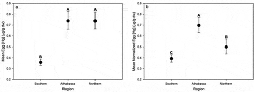
Sentinel species

For a sentinel species to be useful, it needs to be sensitive to exposure to the contaminant of interest so that a measurable biological effect occurs in response to exposure (Cruz-Martinez and Smits 2012). Sensitive and measurable (and robust and repeatable; the measures must be easily distinguished from the “noise” in the system) biological effects are important for early detection of contaminant concentration changes in the ecosystem and for providing potential “markers” or thresholds for regulatory action (Cruz-Martinez and Smits 2012). Sound knowledge of the sentinel species’ biology is also required so that causation of effects can be investigated. Given that contaminants can be transported throughout the ecosystem, exposure routes will vary depending on the species. Species of higher trophic positions within an ecosystem are valuable as sentinel species, as they have the potential to bioaccumulate and biomagnify certain contaminants and can therefore provide insight to ecosystem effects (Cruz-Martinez and Smits 2012).

Feasibility of cost of sample collection and analyses is another important consideration when selecting a sentinel species, not only for practicality, but also for cost efficiency (Cruz-Martinez and Smits 2012). In addition, species that have widespread distribution, but a restricted home range, ensure exposure to local contaminants while allowing site selection to occur to allow optimization of study design (Cruz-Martinez and Smits 2012). It is also important that samples can be easily obtained and that the species is tolerant to interference if the study involves noninvasive or nonlethal sampling (Cruz-Martinez and Smits 2012).

Tree swallows have been used to monitor contaminants in the OS region since the late 1990s, with an even longer history of use in examining effects on ecosystems of environmental contaminants. Table 2 lists the criteria used in the comprehensive evaluation framework for assessing a species’ potential as a sentinel species and summarizes expert judgment for the tree swallow as a case study. This builds upon existing knowledge, including recent experience gained during the JOSM. Many of the tree swallow attributes based on the criteria in Table 2 support a conclusion that they are a robust sentinel species for long-term ambient monitoring of the potential impacts of air pollution in the OS region.

Table 2. Criteria supporting use of the tree swallow as an indicator of OS air pollution impacts.

	Tree swallow rank
Criterion	Low	Medium	High
Robust and reproducible response			✔
Research feasibility/tractability			✔
Response sensitivity			✔
Link to OS			✔
Link to air pollution			✔
Link to OS air pollution			✔
Cost-efficient		✔
“Health-based” measurements possible			✔
Laboratory validation			✔
Noninvasive or nonlethal possible			✔
Regulatory relevance			✔
“Threshold” measurements		✔
Long-term monitoring capability			✔
Power analysis for sample size possible			✔
Human health linkage		✔
Risk assessment/mapping possible		✔
Indigenous knowledge incorporation possible		✔

Notes. The “value” or ability of the tree swallow to fulfill the requirements of the individual criteria is ranked based upon expert judgment. Table S5.1 (Section S5.3 of the supplemental material) provides rationale and supporting citations for these rankings.

Concluding remarks

This critical review attempts to describe the extent of the ECCC science advances in air pollution understanding and links to potential ecosystem responses pertaining to OS development in Alberta, Canada. This work was in support of JOSM, a major, multistakeholder effort. Recognizing that the extent of the monitoring and research that has been conducted during JOSM and by other researchers is greater than what has been covered in this critical review, it is not appropriate to base overall conclusions about OS impacts only on the portion of the work presented here. Furthermore, JOSM (now referred to as OSM) is an ongoing program, and ECCC results reviewed here represent relatively early steps in the research given the long time frame required to advance understanding of the complex scientific questions affecting the OS region.

Important improvements have been made in baseline information across air, water, and wildlife, and, as a result, future monitoring can be expected to be more sensitive and responsive to environmental changes associated with OS development. Monitoring and evaluation of potential sentinel species relevant to air pollutant emissions that have been undertaken have identified approaches for continued monitoring in the OS region. Contaminant exposures have been documented in the aquatic and terrestrial species studied, and biological responses have also been observed. However, attribution of these effects to OS air pollutant emissions in light of other sources and stressors is a significant challenge and knowledge is incomplete. Understanding the significance or implications of these effects also requires further research. In particular, linking water quality throughout the region to OS development and the associated atmospheric emissions, while accounting for natural levels of contaminants, such as PACs due to erosion of bitumen, remains a challenge.

Ongoing research related to the OS region will be able to improve quantification of emissions and atmospheric processes so that areas of potential concern (i.e., where contaminants are being detected in the ecosystem or are projected to be occurring at or near critical loads) can be more reliably characterized and prioritized for enhanced monitoring. This could also include ambient monitoring of pollutants previously not studied, such as intermediate volatility organic species (IVOCs), organic nitrates, organic acids, isocyanic acid, secondary organic aerosols, and large particle (dust) composition.

Increasing the extent that ambient concentration and deposition monitoring of pollutants is actively linked to research undertaken by the other components (i.e., water and wildlife) will be needed to gain a better understanding of the specific role(s) of air emissions in ecological effects. Greater integration will also be necessary to improve understanding of how the elevated amounts of deposition of acidifying and neutralizing compounds, mercury, trace metals, and PACs, that have been identified within 25–50 km of the main surface mining region, move from the points of deposition into the watershed and biota. Similarly, more-integrated studies are needed in order to better understand the origins of the higher levels of mercury in gull eggs in the PAD and the reasons for the observed variability in mercury, metals, and PACs among sampling points across the PAD. In the future, these integrated studies would ideally lead to a much improved understanding of the relationships among the emissions of these pollutants of concern and ecosystem exposures (i.e., deposition, transformation, and uptake) and biological responses. However, atmospheric and multimedia models capable of representing these processes (for PACs and metals) have yet to be applied and tested in the OS region. Acquiring this capacity (e.g., physically based models of PAC emission, transformation, and deposition) will require more research and development, and the importance or priority of obtaining such capacity requires assessment, including new measurement studies that test current knowledge.

To obtain the holistic understanding desired, from air emissions to impacts, many knowledge gaps will need to be filled. Many of these gaps are not unique to the OS but represent ongoing gaps in scientific understanding of relevance to most environmental issues pertaining to pollutant releases to the air (e.g., dry deposition and atmospheric scavenging processes; biological effects of chemical mixtures and of multiple stressors, including effects of low-dose, chronic exposures; multimedia measurement and source attribution of chemical exposures).

The weight of evidence, based upon multiple measurements and data analyses, indicates that atmospheric emissions from complex industrial sources are not well known and are likely being underestimated. This pertains to key toxics generally emitted in small quantities such as PACs and metals, for which emissions are difficult to determine, particularly from fugitive sources; to compounds previously not formally considered, such as low-molecular-weight organic acids and intermediate and semivolatile organic compounds; and to important criteria air contaminants such as VOCs. Given the critical role of accurate knowledge of what is being emitted to scientific understanding of effects (e.g., estimating inputs into ecosystems) and environmental management, addressing the gap in emission knowledge is important.

A scientifically sound sentinel species approach to wildlife monitoring is emerging and becoming viable. However, identification of the appropriate thresholds for meaningful effects (e.g., critical effect sizes), including in aquatic species, that can be sufficiently attributed to OS development activities and air pollutant emissions, and that can be used to predict more serious effects (and additionally in the context of overall cumulative effects), represents an ongoing challenge. Signs of early stress through monitoring are desired; however, thresholds at which adaptive OS management would dictate a response requires attention. As mentioned above, more-integrated studies are needed to potentially advance understanding.

Some of the priorities for ongoing and enhanced monitoring to advance scientific understanding and potentially inform adaptive management include multimedia, multistressor monitoring of conditions and changes and their sources in the PAD; deposition and ecosystem changes in areas where current best estimates are that critical loads for acidic deposition are being exceeded; tracking of changes in contaminant levels in plant and animal tissues, particularly those consumed by humans where some levels have led to consumption advisories; and improved tracking and independent validation of atmospheric emissions of a wide range of compounds from multiple sources, including key fugitive sources that contribute to the large burden of chemically complex dust in the near-field region and VOCs (IVOCs) and PACs.

Glossary of terms

ALKA	=	C4+ alkanes
alk-DBTs	=	alkylated dibenzothiophenes
alk-PAHs	=	alkylated PAHs
APEI	=	Air Pollutant Emissions Inventory
AOP	=	adverse outcome pathway
AR	=	Athabasca River
AROM	=	di/trisubstituted aromatics
AURAMS	=	A Unified Regional Air-quality Modeling System
BTEX	=	benzene, toluene, ethylbenzene, and xylenes
CACs	=	criteria air contaminants
CCME	=	Canadian Council for Ministers of the Environment
CEMA	=	Cumulative Environmental Management Association
CES	=	critical effect sizes
CLRTAP	=	Convention on Long-Range Transboundary Air Pollution
CNRL	=	Natural Resources Limited Horizon Facility
COCs	=	contaminants of concern
DBTs	=	dibenzothiophenes
DOC	=	dissolved organic carbon
ECCC	=	Environment and Climate Change Canada
EFs	=	emission factors
EPA	=	U.S. Environmental Protection Agency
EPT	=	Ephemeroptera (mayfly), Plecoptera (stonefly) and Trichoptera (caddisfly) (EPT)
EROD	=	ethoxyresorufin-O-deethylase
FA	=	HCOOH/formic acid
FAB	=	First-Order Acidity Balance
GEM	=	Global Environmental Multiscale
GEM-MACH	=	Global Environmental Multiscale–Modeling Air-quality and CHemistry model
GHGs	=	green house gases
GHGRP	=	Greenhouse Gas Reporting Program
HNCO	=	isocyanic acid
IJC	=	International Joint Commission
IKL	=	Imperial Kearl Oil Sands Mine
IVOCs	=	intermediate volatile organic compounds
JOSM	=	Joint Oil Sands Monitoring (Canada—Alberta)
LAR	=	Lower Athabasca River
LMWOAs	=	low-molecular-weight organic acids
MeHg	=	methyl mercury
NEG-ECP	=	New England Governors–Eastern Canadian Premiers
NPRI	=	National Pollutant Release Inventory
OMI	=	ozone monitoring instrument
ON	=	organonitrates
OS	=	oil sands
PACs	=	polycyclic aromatic compounds
PAD	=	Peace-Athabasca Delta
PAHs	=	polycyclic aromatic hydrocarbons
PM or TPM	=	particulate matter
POD	=	phytotoxic ozone dose
pON	=	particulate organonitrate compounds
POPs	=	persistent organic pollutants
Ramsar Convention	=	The Convention on Wetlands of International Importance
RSC	=	Royal Society of Canada
SAJ	=	Shell Albian Sands and Jackpine Mines
SAU	=	Syncrude Aurora Facility
diss As	=	dissolved As
diss Se	=	dissolved Se
SLCPs	=	short-lived climate pollutants
SMB	=	Simple Mass Balance
SML	=	Syncrude Mildred Lake Facility
SOA	=	secondary organic aerosol
SPMD	=	semipermeable membrane device
SSWC	=	Steady-State Water Chemistry
SVOCs	=	semivolatile organic compounds
SUN	=	Suncor Millenium and Steepbank
TEEM	=	Terrestrial Environmental Effects Monitoring
TEK	=	traditional ecological knowledge
TERRA	=	Top-down Emission Rate Retrieval Algorithm
TES	=	tropospheric emission spectrometer
THg	=	total mercury
TOLU	=	monosubstituted aromatic
TP	=	total phosphate
UNECE LRTAP	=	United Nations Economic Commission for Europe Long-Range Transboundary Air Pollution
UNESCO	=	United Nations Educational, Scientific, and Cultural Organization
UNFCCC	=	United Nations Framework Convention on Climate Change
VOC	=	volatile organic compounds
WBEA	=	Wood Buffalo Environmental Association
WMO-UNEP	=	World Meteorological Organisation–United Nations Environmental Protection

Acknowledgment

The authors thank Stoyka Netcheva, Sean Rowe, Andrea Darlington, Julie Narayan, Mark Shepard, and Chris McLinden from the Air Quality Research Division of Environment and Climate Change Canada; Kim Fernie, Catherine Soos, Craig Hebert, Phil Thomas, Lukas Mundy, Céline Boutin, David Carpenter, and Julie Bilodeau from the Wildlife and Landscape Science Directorate; and Joseph Culp and Ian Droppo from the Water Science and Technology Directorate of Environment and Climate Change Canada for their contributions.

Supplemental data for this paper can be accessed on the publisher’s website.

Additional information

Funding

The monitoring reviewed in this paper was funded under the Oil Sands Monitoring Program and through the Environment and Climate Change Canada Air Pollution program.

Notes on contributors

J.R. Brook

Dr. J.R. Brook recently joined the faculty at the University of Toronto after a 27 career as a scientist in the Air Quality Research Division of Environment and Climate Change Canada.

References

- Achten, C., and J. T. Andersson. 2015. Overview of polycyclic aromatic compounds (PAC). Polycycl. Aromat. Compd. 35 (2–4):177–86. doi:10.1080/10406638.2014.994071.
- AEP. 2016. Joint oil sands monitoring program emissions inventory full report. Accessed March 22, 2019. https://open.alberta.ca/publications/9781460125658.
- Aherne, J. 2011. Uncertainty in critical load exceedance (UNCLE): Critical loads uncertainty and risk analysis for Canadian forest ecosystems. Canadian Council of Ministers of the Environment, report PN XXXX, 22.
- Aherne, J., and M. Posch. 2013. Impacts of nitrogen and sulphur deposition on forest ecosystem services in Canada. Curr. Opin. Environ. Sustain. 5 (1):108–15. doi:10.1016/j.cosust.2013.02.005.
- Akingunola, A., P. A. Makar, J. Zhang, A. Darlington, S.-M. Li, M. Gordon, M. D. Moran, and Q. Zheng. 2018. A chemical transport model study of plume rise and particle size distribution for the Athabasca oil sands. Atmos. Chem. Phys. 18:8667–88. doi:10.5194/acp-18-8667-2018.
- Alberta Biodiversity Monitoring Institute, Canada. 2019. Our vision and mission. Accessed January 9, 2019. https://www.abmi.ca/home/about-us/our-vision-mission.html.
- Alberta Energy Regulator, Canada. 2017. Crude bitumen production. Accessed March 22, 2019. https://www.aer.ca/providing-information/data-and-reports/statistical-reports/crude-bitumen-production.
- Alberta Environment and Parks. 2016. Air pollutant and GHG emissions from mine faces and tailings ponds (second draft). Report prepared by Stantec Consulting Ltd., Clearstone Engineering Ltd and Intrisik Environmental Science Inc, 413.
- Alberta Environment and Sustainable Resource Development. 2013. Report on the inventory of oil sands inventories. Internal Report, 88, April.
- Alexander, A. C., and P. A. Chambers. 2016. Assessment of seven Canadian rivers in relation to stages in oil sands industrial development, 1972-2010. Environ. Rev. 24 (4):484–94. doi:10.1139/er-2016-0033.
- Alexander, A. C., P. A. Chambers, and D. S. Jeffries. 2017. Episodic acidification of 5 rivers in Canada‘s oil sands during snowmelt: A 25-year record. Sci. Total Environ. 599-600:739–49. doi:10.1016/j.scitotenv.2017.04.207.
- Andrew, M. E., M. A. Wulder, and T. A. Nelson. 2014. Potential contributions of remote sensing to ecosystem service assessments. Prog. Phys. Geogr. 38 (3):328–52. doi:10.1177/0309133314528942.
- Arciszewski, T. J., K. R. Munkittrick, B. W. Kilgour, H. M. Keith, J. E. Linehan, and M. E. McMaster. 2017b. Increased size and relative abundance of migratory fishes observed near the Athabasca oil sands. Facets 2:833–58. doi:10.1139/facets-2017-0028.
- Arciszewski, T. J., K. R. Munkittrick, G. J. Scrimgeour, M. G. Dubé, F. J. Wrona, and R. R. Hazewinkel. 2017a. Using adaptive processes and adverse outcome pathways to develop meaningful, robust, and actionable environmental monitoring programs. Integr. Environ. Assess. Manag. 13 (5):877–91. doi:10.1002/ieam.1938.
- Arey, J., W. P. Harger, D. Helmig, and R. Atkinson. 1992. Bioassay-directed fractionation of mutagenic PAH atmospheric photooxidation products and ambient particulate extracts. Mutat. Res. Lett. 281 (1):67–76. doi:10.1016/0165-7992(92)90038-J.
- Azuma, K., I. Uchiyama, S. Uchiyama, and N. Kunugita. 2016. Assessment of inhalation exposure to indoor air pollutants: Screening for health risks of multiple pollutants in Japanese dwellings. Environ. Res. 145:39–49. doi:10.1016/j.envres.2015.11.015.
- Baray, S., A. Darlington, M. Gordon, K. L. Hayden, A. Leithead, S.-M. Li, P. S. K. Liu, R. L. Mittermeier, S. G. Moussa, J. O‘Brien, et al. 2018. Quantification of methane sources in the Athabasca Oil Sands Region of Alberta by aircraft mass balance. Atmos. Chem. Phys. 18:7361–78. doi:10.5194/acp-18-7361-2018.
- Bari, M., W. Kindzierski, and S. Cho. 2014. A wintertime investigation of atmospheric deposition of metals and polycyclic aromatic hydrocarbons in the Athabasca Oil Sands region, Canada. Sci. Total Environ. 485–486:180–92. doi:10.1016/j.scitotenv.2014.03.088.
- Bickerton, G., J. W. Roy, R. A. Frank, J. Spoelstra, G. Langston, L. Grapentine, and L. M. Hewitt. 2018. Assessments of groundwater influence on select river systems in the oil sands region of Alberta. Oil Sands Monitoring Program Technical Report Series No. 1.5, 32. ISBN 978-1-4601-4029-1.
- Bilodeau, J. C., J. M. Gutierrez-Villagomez, L. E. Kimpe, P. J. Thomas, B. D. Pauli, V. L. Trudeau, and J. M. Blais. 2019. Toxicokinetics and bioaccumulation of polycyclic aromatic compounds in wood frog tadpoles (Lithobates sylvaticus) exposed to Athabasca oil sands sediment. Aquat. Toxicol. 207:217–22. doi:10.1016/j.aquatox.2018.11.006.
- Birks, S. J., S. Cho, E. Taylor, Y. Yi, and J. J. Gibson. 2017. Characterizing the PAHs in surface waters and snow in the Athabasca region: Implications for identifying hydrological pathways of atmospheric deposition. Sci. Total Environ. 603–604:570–83. doi:10.1016/j.scitotenv.2017.06.051.
- Blum, J. D., M. W. Johnson, J. D. Gleason, J. D. Demers, M. S. Landis, and S. Krupa. 2012. Mercury concentration and isotopic composition of epiphytic tree lichens in the Athabasca Oil Sands Region. In Alberta Oil Sands: Energy, Industry and the Environment, ed. K. E. Percy, 373–90. Oxford, UK: Elsevier.
- Bobbink, R., K. Hicks, J. Galloway, T. Spranger, R. Alkemade, M. Ashmore, M. Bustamante, S. Cinderby, E. Davidson, F. Dentener, et al. 2010. Global assessment of nitrogen deposition effects on terrestrial plant diversity: A synthesis. Ecol. Appl. 20 (1):30–59. doi:10.1890/08-1140.1.
- Bosch, C., A. Andersson, M. Krusa, C. Bandh, I. Hovorkova, J. Klanova, T. Knowles, R. D. Pancost, R. P. Evershed, and O. Gustafsson. 2015. Source apportionment of polycyclic aromatic hydrocarbons in central European soils with compound-specific triple isotopes (_13C, _14C, and _2H). Environ. Sci. Technol. 49 (13):7657–65. doi:10.1021/acs.est.5b01190.
- Boutin, C., and D. J. Carpenter. 2017. Assessment of wetland/upland vegetation communities and evaluation of soil-plant contamination by polycyclic aromatic hydrocarbons and trace metals in regions near oil sands mining in Alberta. Sci. Total Environ. 576:829–39. doi:10.1016/j.scitotenv.2016.10.062.
- Bradley, P. M., C. A. Journey, J. P. Berninger, D. T. Button, J. M. Clark, S. R. Corsi, L. A. DeCicco, K. G. Hopkins, B. J. Huffman, N. Nakagaki, et al. 2019. Mixed-chemical exposure and predicted effects potential in wadeable southeastern USA streams. Sci. Total Environ. 655:70–83. doi:10.1016/j.scitotenv.2018.11.186.
- Brady, J. M., T. A. Crisp, S. Collier, T. Kuwayama, S. D. Forestieri, V. Perraud, Q. Zhang, M. J. Kleeman, C. D. Cappa, and T. H. Bertram. 2014. Real-time emission factor measurements of isocyanic acid from light duty gasoline vehicles. Environ. Sci. Technol. 48 (19):11405–12. doi:10.1021/es504354p.
- Brander, S. M., A. D. Biales, and R. E. Connon. 2017. The role of epigenomics in aquatic toxicology. Environ. Toxicol. Chem. 36 (10):2565–73. doi:10.1002/etc.3930.
- Briggs, G. A. 1985. Analytical parameterizations of diffusion: The convective boundary layer. J. Clim. Appl. Meteorol. 24 (11):1167–86. doi:10.1175/1520-0450(1985)024≤1167:APODTC≥2.0.CO;2.
- Briggs, G. A. 1969. Plume rise. Springfield, Virginia: U.S. Atomic Energy Commission, Division of Technical Information.
- Briggs, G. A. 1975. Plume rise predictions. In Lectures on air Pollution and environmental impact analyses, ed, D. Haugen, 59–111. Boston: University of Chicago Press.
- Briggs, G. A. 1984. Plume rise and buoyancy effects, atmospheric sciences and power production. Oak Ridge, USA: Technical Information Center, U.S. Dept. of Energy.
- Brook, J. R., and M. D. Moran. 2000. International workshop on techniques and problems in modelling size-distributed aerosol formation and composition. Atmos. Environ. 34:1153–54.
- Campbell, H. E., . D., R. Kindopp, S. MacMillan, P. Martin, E. Neugebauer, L. Patterson, and J. Shatford. 2013. Mercury trends in colonial waterbird eggs downstream of the oil sands region of Alberta, Canada. Environ. Sci. Technol. 47 (20):11785–92. doi:10.1021/es402542w.
- Carlton, A. G., B. J. Turpin, K. E. Altieri, S. Seitzinger, A. Reff, H. J. Lim, and B. Ervens. 2007. Atmospheric oxalic acid and SOA production from glyoxal: Results of aqueous photooxidation experiments. Atmos. Environ. 41 (35):7588–602. doi:10.1016/j.atmosenv.2007.05.035.
- Carou, S., I. Dennis, J. Aherne, R. Ouimet, P. A. Arp, S. A. Watmough, I. DeMerchant, M. Shaw, B. Vet, V. Bouchet, et al. 2008. A national picture of acid deposition critical loads for forest soils in Canada. Canadian Council of Ministers of the Environment, PN 1412, 6.
- CCME, Canada. 1999. Canadian sediment quality guidelines for the protection of aquatic life. Accessed January 9, 2019. http://ceqg-rcqe.ccme.ca/download/en/312.
- CCME, Canada. 2003. Canadian sediment quality guidelines for the protection of aquatic life. Accessed March 22, 2019. http://ceqg-rcqe.ccme.ca/download/en/221.
- Chambers, P. A., A. Alexander Trusiak, J. Kirk, C. Manzano, D. Muir, C. Cooke, and R. Hazewinkel. 2018. Surface water quality of lower athabasca river tributaries. Oil Sands Monitoring Program Technical Report Series No. 1.3, 34. ISBN 978-1-4601-4027-7.
- Cheng, Y., S.-M. Li, M. Gordon, and P. Liu. 2018. Size distribution and coating thickness of black carbon from the Canadian oil sands operations. Atmos. Chem. Phys. 18:2653–67. doi:10.5194/acp-18-2653-2018.
- Cheng, Y., S.-M. Li, J. Liggio, M. Gordon, A. Darlington, Q. Zheng, P. Liu, and M. Wolde. 2019. Top down determination of black carbon emission from oil sands facilities in Alberta, Canada using aircraft measurements. Environ. Scie. Technol..
- Cho, S., K. Sharma, B. Brassard, and R. Hazewinkel. 2014. Polycyclic aromatic hydrocarbon deposition in the snowpack of the Athabasca oil sands region of Alberta, Canada. Water. Air Soil Pollut. 225 (5):1910. doi:10.1007/s11270-014-1910-4.
- Clarkson, T. W. 1993. Mercury: Major issues in environmental health. Environ. Health Perspect. 100:31–38. doi:10.1289/ehp.9310031.
- Clemente, J. S., and P. M. Fedorak. 2005. A review of the occurrence, analyses, toxicity, and biodegradation of naphthenic acids. Chemosphere 60 (5):585–600. doi:10.1016/j.chemosphere.2005.02.065.
- CLRTAP. 2017. Manual on methodologies and criteria for modelling and mapping critical loads and levels and air pollution effects, risks and trends. Accessed March 22, 2019. http://icpmapping.org/.
- Cooke, C. A., J. L. Kirk, D. C. G. Muir, J. A. Wiklund, X. Wang, A. Gleason, and M. S. Evans. 2017. Spatial and temporal patterns in trace element deposition to lakes in the Athabasca oil sands region (Alberta, Canada). Environ. Res. Lett. 12:124001.
- Cruz-Martinez, L., K. J. Fernie, C. Soos, T. Harner, F. Getachew, and J. Smits. 2015. Detoxification, endocrine, and immune responses of tree swallow nestlings naturally exposed to air contaminants from the Alberta oil sands. Sci. Total Environ. 502:8–15. doi:10.1016/j.scitotenv.2014.09.008.
- Cruz-Martinez, L., and J. Smits. 2012. Potential to use animals as monitors of ecosystem health in the Oil Sands Region. Environment. doi:10.7939/R31C4G.
- Culp, J. M., I. G. Droppo, P. Di Cenzo, A. Alexander-Trusiak, D. J. Baird, S. Beltaos, B. Bickerton, B. Bonsal, B. Rb, P. A. Chambers, et al. 2018a. Synthesis report for the water component, Canada-Alberta joint oil sands monitoring: Key findings and recommendations. Oil Sands Monitoring Program Technical Report Series No. 1.1, 46. ISBN 978-1-4601-4025-3.
- Culp, J. M., N. E. Glozier, D. J. Baird, F. J. Wrona, R. B. Brua, A. L. Ritcey, D. L. Peters, R. Casey, C. B. Choung, C. J. Curry, et al. 2018b. Assessing ecosystem health in benthic macroinvertebrate assemblages of the athabasca river main stem, tributaries, and peace-athabasca delta. Oil Sands Monitoring Technical Report Series No. 1.7, 82. ISBN: 978-1-4601-4155-7.
- Davies, M. J. E. 2012. Air quality modelling in the Athabasca Oil Sands Region. In Alberta Oil Sands: Energy, industry and the environment, ed. K. E. Percy, 267–309. Oxford, UK: Elsevier.
- De Araujo Barbosa, C. C., P. M. Atkinson, and J. A. Dearing. 2015. Remote sensing of ecosystem services: A systematic review. Ecol. Indic. 52:430–43. doi:10.1016/j.ecolind.2015.01.007.
- Dickson, W. 1978. Some effects of acidification on Swedish lakes. Verh. Internat Verein. Limnol. 20:851–56.
- Dolgova, S., D. Crump, E. Porter, K. Williams, and C. E. Hebert. 2018a. Stage of development affects dry weight mercury concentrations in bird eggs: Laboratory evidence and adjustment method. Environ. Toxicol. Chem. 37 (4):1168–74. doi:10.1002/etc.4066.
- Dolgova, S., B. N. Popp, K. Courtoreille, R. H. M. Espie, B. Maclean, J. R. Straka, G. R. Tetreault, S. Wilkie, and C. E. Herbert. 2018b. Spatial trends in a biomagnifying contaminant: Application of amino acid compound–Specific stable nitrogen isotope analysis to the interpretation of bird mercury levels. Environ. Toxicol. Chem. 37 (5):1466–75. doi:10.1002/etc.4113.
- Dowdeswell, L., P. Dillon, S. Ghoshal, A. Miall, J. Rasmussen, and J. P. Smol. 2010. A foundation for the future: Building an environmental monitoring system for the system for the Oil Sands. Gatineau: Environment Canada.
- Droppo, I. G., P. Di Cenzo, J. Power, C. Jaskot, P. Chambers, A. C. Alexander, J. Kirk, and D. Muir. 2018b. Temporal and spatial trends in riverine suspended sediment and associated polycyclic aromatic compounds (PAC) within the Athabasca Oil Sands Region. Sci. Total Environ. 626:1382–93. doi:10.1016/j.scitotenv.2018.01.105.
- Droppo, I. G., T. Prowse, B. Bonsal, Y. Dibike, S. Beltaos, B. Krishnappan, H.-L. Eum, S. Kashyap, A. Sakibaeinia, and A. Gupta. 2018a. Regional Hydro-climatic and Sediment Modelling for the Lower Athabasca River Oil Sands Region. Oil Sands Monitoring Program Technical Report Series No. 1.6, 89. ISBN 978-1-4601-4030-7.
- Dziedek, C., W. Härdtle, G. von Oheimb, and A. Fichtner. 2016. Nitrogen addition enhances drought sensitivity of young deciduous tree species. Front. Plant Sci. 77. doi:10.3389/fpls.2016.01100.
- Earl, S. R., H. M. Valett, and J. R. Webster. 2006. Nitrogen saturation in stream ecosystems. Ecology 87 (12):3140–51.
- ECCC, Environment and Climate Change Canada. 2016. Canada’s Black carbon inventory, 2016 edition. Accessed April 5, 2019. https://ec.gc.ca/air/3F796B41-0B87-4C14-B76D-899D23CD0295/Black%20Carbon%202016-EN-Final.pdf.
- Eldering, A., and G. R. Cass. 1996. Source-oriented model for air pollutant effects on visibility. J. Geophys. Res. Atmos. 1011 (14):19343–70. doi:10.1029/95JD02928.
- Environment Canada. 2011. Eds. F.J. Wrona, P. di Cenzo, and K. Schaefer. Integrated monitoring plan for the oil sands – Expanded geographic extent for water quality and quantity, aquatic biodiversity and effects, and acid sensitive lake component. http://publications.gc.ca/collections/collection_2011/ec/En14-49-2011-eng.pdf.
- Environment Canada, Canada. 2016. Environment and climate change Canada & Alberta environment and parks): Joint oil sands monitoring program emissions inventory compilation. Accessed April 5, 2019. https://open.alberta.ca/publications/9781460125658.
- Ervens, B., G. Feingold, G. J. Frost, and S. M. Kreidenweis. 2004. A modeling of study of aqueous production of dicarboxylic acids: 1. Chemical pathways and speciated organic mass production. J. Geophys. Res. Atmos. 109 (15):15201–20. doi:10.1029/2003JD004387.
- Evans, M. S., and A. Talbot. 2012. Investigations of mercury concentrations in walleye and other fish in the Athabasca River ecosystem with increasing oil sands developments. Environ. Monit. Assess. 14 (7):1989–2003. doi:10.1039/c2em30132f.
- Fernie, K. J., L. Cruz-Martinez, L. Peters, V. Palace,And, and J. Smits. 2016. Inhaling benzene, toluene, nitrogen dioxide, and sulfur dioxide, disrupts thyroid function in captive American kestrels (Falco sparverius). Environ. Sci. Technol. 50 (20):11311–18. doi:10.1021/acs.est.6b03026.
- Fernie, K. J., S. C. Marteinson, D. Chen, A. Eng, T. Harner, J. Smits, and C. Soos. 2018a. Elevated exposure, uptake and accumulation of polycyclic aromatic hydrocarbons by nestling tree swallows (Tachycineta bicolor) through multiple exposure routes in active mining-related areas of the Athabasca oil sands region. Sci. Total Environ. 624:250–61. doi:10.1016/j.scitotenv.2017.12.123.
- Fernie, K. J., S. C. Marteinson, D. Chen, L. Peters, V. Palace, and J. Smits. 2019. Changes in thyroid function of nestling tree swallows (Tachycineta bicolor) in relation to polycyclic aromatic compounds and other stressors in the Athabasca Oil Sands. Environ. Res. 169:464–75. doi:10.1016/j.envres.2018.11.031.
- Fernie, K. J., S. C. Martienson, C. Soos, D. Chen, L. Cruz-Martinez, and J. Smits. 2018. Reproductive and developmental changes in tree swallows (Tachycineta bicolor) are influenced by multiple stressors, including polycyclic aromatic compounds, in the Athabasca Oil Sands. Environ. Pollut. 238:931–41. doi:10.1016/j.envpol.2018.03.074.
- Fioletov, V. E., C. Mclinden, N. Krotkov, and C. Li. 2015. Lifetimes and emissions of SO2 from point sources estimated from OMI. Geophys. Res. Lett. 42:6. doi:10.1002/2015GL063148.
- Fioletov, V. E., C. A. McLinden, S. K. Kharol, N. A. Krotkov, C. Li, J. Joiner, M. D. Moran, R. Vet, A. J. H. Visschedijk, and H. A. C. Denier van der Gon. 2017. Multi-source SO2 emission retrievals and consistency of satellite and surface measurements with reported emissions. Atmos. Chem. Phys. 17:12597–616. doi:10.5194/acp-17-12597-2017.
- Fox, D. G. 1981. Judging air quality model performance - summary of the AMS Workshop on Dispersion Model Performance, Woods Hole, Mass., 8-11 September 1980. Bull. Am. Met. Soc. 62:599–609. doi:10.1175/1520-0477(1981)062<0599:JAQMP>2.0.CO;2.
- Fox, D. G. 1984. Uncertainty in air quality modelling – A summary of the AMS Workshop on Quantifying and Communicating Model Uncertainty, Woods Hole, Mass., September 1982. Bull. Am. Met. Soc. 65:27–36. doi:10.1175/1520-0477(1984)065<0027%3AUIAQM>2.0.CO%3B2.
- Gagné, F., A. Bruneau, P. Turcotte, C. Gagnon, and E. Lacaze. 2017. An investigation of the immunotoxicity of oil sands processed water and leachates in trout leukocytes. Ecotoxicol. Environ. Saf. 141:43–51. doi:10.1016/ecoenv.2017.03.012.
- Gagné, F., M. Douville, C. André, T. Debenest, A. Talbot, J. Sherry, L. M. Hewitt, R. A. Frank, M. E. McMaster, J. Parrot, et al. 2012. Differential changes in gene expression in rainbow trout hepatocytes exposed to extracts of oil sands process-affected water and the Athabasca River. Comp. Biochem. Physiol. C. 155 (4):551–59. doi:10.1016/j.cbpc.2012.01.004.
- Galarneau, E., B. P. Hollebone, Z. Yang, and J. Schuster. 2014. Preliminary measurement-based estimates of PAH emissions from oil sands tailings ponds. Atmos. Environ. 97:332–35. doi:10.1016/j.atmosenv.2014.08.038.
- Gentes, M. L., A. McNabb, C. Waldner, and J. Smits. 2007. Increased thyroid hormone levels in tree swallows (Tachycineta bicolor) on reclaimed wetlands of the Athabasca oil sands. Arch. Environ. Contam. Toxicol. 53 (2):287–92. doi:10.1007/s00244-006-0070-y.
- Gerner, N. V., M. Koné, M. S. Ross, A. Pereira, A. C. Ulrich, J. W. Martin, and M. Liess. 2017. Stream invertebrate community structure at Canadian Oil Sands development is linked to concentration of bitumen-derived contaminants. Sci. Total Environ. 575:1005–13. doi:10.1016/j.scitotenv.2016.09.169.
- Glozier, N. E., K. Pippy, L. Levesque, A. Ritcey, B. Armstrong, O. Tobin, C. A. Cooke, M. Conly, L. Dirk, C. Epp, et al. 2018. Surface water quality of the athabasca, peace and slave rivers and riverine waterbodies within the Peace-Athabasca Delta. Oil Sands Monitoring Program Technical Report Series No. 1.4, 64. ISBN: 978-1-4601-4152-6.
- Godwin, C. M., R. M. Barclay, and J. E. G. Smits. 2019. Tree swallow (Tachycineta bicolor) nest success and nestling growth near oilsands mining operations in Northeastern Alberta. Can. J. Zool. 1–41. doi:10.1139/cjz-2018-0247.
- Gong, W., A. P. Dastoor, V. S. Bouchet, S. Gong, P. A. Makar, M. D. Moran, B. Pabla, S. Menard, L.-P. Crevier, S. Cousineau, et al. 2006. Cloud processing of gases and aerosols in a regional air quality model (AURAMS). Atmos. Res. 82 (1–2):248–75. doi:10.1016/j.atmosres.2005.10.012.
- Gordon, M., S.-M. Li, R. Staebler, A. Darlington, K. Hayden, J. O‘Brien, and M. Wolde. 2015. Determining air pollutant emission rates based on mass balance using airborne measurement data over the Alberta oil sands operations. Atmos. Meas. Tech. 8 (3745–3765):2015. doi:10.5194/amt-8-3745-2015.
- Gordon, M., P. Makar, R. Staebler, J. Zhang, A. Akingunola, W. Gong, and S.-M. Li. 2018. A comparison of plume rise algorithms to stack plume measurements in the Athabasca Oil Sands. Atmos. Chem. Phys. 18:14695–714. doi:10.5194/acp-18-14695-2018.
- Government of Canada, Canada. 2019a. National pollutant release inventory. Accessed March 22, 2019. https://www.canada.ca/en/services/environment/pollution-waste-management/national-pollutant-release-inventory.html.
- Government of Canada, Canada. 2019b. Canada’s air pollutant emissions inventory. Accessed March 22, 2019. https://open.canada.ca/data/en/dataset/fa1c88a8-bf78-4fcb-9c1e-2a5534b92131.
- Graney, J. R., M. S. Landis, K. J. Puckett, W. B. Studabaker, E. S. Edgerton, A. H. Legge, and K. E. Percy. 2017. Differential accumulation of PAHs, elements, and Pb isotopes by five lichen species from the Athabasca Oil Sands Region in Alberta, Canada. Chemosphere 184:700–10. doi:10.1016/j.chemosphere.2017.06.036.
- Hanha, S. R. 1988. Air quality model evaluation and uncertainty. J. Air Poll. Cont. Assoc. 38 (4):406–12. doi:10.1080/08940630.1988.10466390.
- Harman, C., E. Farmen, and K. E. Tollefsen. 2010. Monitoring North Sea oil production discharges using passive sampling devices coupled with in vitro bioassay techniques. J. Environ. Monit. 12 (9):1699–708. doi:10.1039/C0EM00147C.
- Harms, N. J., G. D. Fairhurst, G. R. Bortolotti, and J. E. G. Smits. 2010. Variation in immune function, body condition, and feather corticosterone in nestling Tree Swallows (Tachycineta bicolor) on reclaimed wetlands in the Athabasca oil sands, Alberta, Canada. Environ. Pollut. 158 (3):841–48. doi:10.1016/j.envpol.2009.09.025.
- Harner, T., C. Rauert, D. Muir, J. Schuster, Y.-M. Hsu, L. Zhang, G. Marson, J. G. Watson, J. Ahad, S. Cho, et al. 2018. Air synthesis review on polycyclic aromatic compounds in the Oil Sands Region. Environ Rev 26 (4):430–68. doi:10.1139/er-2018-0039.
- Hebert, C. 2019. The river runs through it: The Athabasca River delivers mercury to aquatic birds breeding far downstream. PLoS ONE 14 (4):e0206192 doi:10.1371/journal.pone.0206192.
- Hebert, C., W. Nordstrom, and L. Shutt. 2010. Colonial waterbirds nesting on Egg Island, Lake athabasca, 2009. Can. Field-Naturalist 124:49–53. doi:10.22621/cfn.v124i1.1029.
- Hebert, C. E., D. V. C. Weseloh, S. Macmillan, D. Campbell, and W. Nordstrom. 2011. Metals and polycyclic aromatic hydrocarbons in colonial waterbird eggs from Lake Athabasca and the Peace-Athabasca Delta, Canada. Environ. Toxicol. Chem. 30 (5):1178–83. doi:10.1002/etc.489.
- Hersikorn, B. D., J. J. H. Ciborowski, and J. Smits. 2010. The effects of oil sands wetlands on wood frogs (Rana sylvatica). Toxicol. Environ. Chem. 92 (8):1513–27. doi:10.1080/02772240903471245.
- Himanen, M., P. Prochazka, K. Hänninen, and A. Oikari. 2012. Phytotoxicity of low-weight carboxylic acids. Chemosphere 88 (4):426–31. doi:10.1016/j.chemosphere.2012.02.058.
- Hsu, Y. M. 2013. Trends in passively-measured ozone, nitrogen dioxide and sulfur dioxide concentrations in the Athabasca Oil Sands Region of Alberta, Canada. Aerosol Air Qual. Res. 13:1448–63. doi:10.4209/aaqr.2012.08.0224.
- Hsu, Y.-M., T. Harner, H. Li, and P. Fellin. 2015. PAH measurements in air in the Athabasca oil sands region. Environ. Sci. Technol. 49 (9):5584–92. doi:10.1021/acs.est.5b00178.
- Jacques, D. R., and A. H. Legge. 2012. Ecological analogues for biomonitoring industrial sulfur emissions in the Athabasca Oil Sands Region, Alberta, Canada. Chapter 10. In Alberta Oil Sands: Energy, industry and the environment, ed. K. E. Percy, 219–41. Oxford, UK: Elsevier.
- Jariyasopit, N., Y. Zhang, J. W. Martin, and T. Harner. 2018. Comparison of polycyclic aromatic compounds in air measured by conventional passive air samplers and passive dry deposition samplers and contributions from petcoke and oil sands ore. Atmos. Chem. Phys. 18:9161–71. doi:10.5194/acp-18-9161-2018.
- Jautzy, J. J., J. M. Ahad, C. Gobeil, A. Smirnoff, B. D. Barst, and M. M. Savard. 2015. Isotopic evidence for oil sands petroleum coke in the Peace–Athabasca Delta. Environ. Sci. Technol. 49 (20):12062–70. doi:10.1021/acs.est.5b03232.
- Jeffries, D. S., R. G. Semkin, J. J. Gibson, and I. Wong. 2010. Recently surveyed lakes in northern Manitoba and Saskatchewan, Canada: Characteristics and critical loads of acidity. J. Limnol. 69 (Suppl. 1):45–55. doi:10.4081/jlimnol.2010.s1.45.
- Joint Canada-Alberta Implementation Plan for Oil Sands Monitoring. 2012. Accessed April 5, 2019. http://www.ec.gc.ca/Scitech/D0AF1423-351C-4CBC-A990-4ADA543E7181/COM1519_Final%20OS%20Plan_02.pdf.
- JOSM, Canada. 2016. Joint oil sands monitoring program emissions inventory report. Accessed January 9, 2019. https://www.canada.ca/en/environment-climate-change/services/science-technology/publications/joint-oil-sands-monitoring-emissions-report.html.
- Jung, K., and S. X. Chang. 2012. Four years of simulated N and S depositions did not cause N saturation in a mixedwood boreal forest ecosystem in the Oil Sands Region in Northern Alberta, Canada. For. Ecol. Manag. 280:62–70. doi:10.1016/j.foreco.2012.06.002.
- Kang, E., M. J. Root, D. W. Toohey, and W. H. Brune. 2007. Introducing the concept of Potential Aerosol Mass (PAM). Atmos. Chem. Phys. 7:5727–44. doi:10.5194/acp-7-5727-2007.
- Kelly, E. N., D. W. Schindler, P. V. Hodson, J. W. Short, R. Radmanovich, and C. C. Nielsen. 2010. Oil Sands development contributes elements toxic at low concentrations to the Athabasca River and its tributaries. Proc. Natl. Acad. Sci. U.S.A. 107:16178–83. doi:10.1073/pnas.1008754107.
- Kelly, E. N., J. W. Short, D. W. Schindler, P. V. Hodson, M. Ma, A. K. Kwan, and B. L. Fortin. 2009. Oil Sands development contributes polycyclic aromatic compounds to the Athabasca River and its tributaries. Proc. Natl. Acad. Sci. U.S.A. 106 (52):22346–51. doi:10.1073/pnas.0912050106.
- Kerr, J. T., and M. Ostrovsky. 2003. From space to species: Ecological applications for remote sensing. Trends Ecol. Evol. 18 (6):299–305. doi:10.1016/S0169-5347(03)00071-5.
- Keyte, I. J., R. M. Harrison, and G. Lammel. 2013. Chemical reactivity and long-range transport potential of polycyclic aromatic hydrocarbons - a review. Chem. Soc. Rev. 42 (24):9333–91. doi:10.1039/c3cs60147a.
- Khare, P., N. Kumar, K. M. Kumari, and S. S. Srivastava. 1999. Atmospheric formic and acetic acids: An overview. Rev. Geophys. 37 (2):227–48. doi:10.1029/1998RG900005.
- Kirk, J., D. Muir, C. Manzano, C. Cooke, J. Wiklund, A. Gleason, J. Summers, J. Smol, and J. Kurek. 2018. Atmospheric deposition to the Athabasca Oil Sands Region using snowpack measurements and dated lake sediment cores. Oil Sands Monitoring Program Technical Report Series No. 1.2, 43. ISBN 978-1-4601-4026-0.
- Kirk, J. L., D. C. G. Muir, A. Gleason, X. Wang, G. Lawson, R. A. Frank, I. Lehnherr, and F. Wrona. 2014. Atmospheric deposition of mercury and methylmercury to landscapes and waterbodies of the Athabasca Oil Sands Region. Environ. Sci. Technol. 48 (13):7374–83. doi:10.1021/es500986r.
- Knox, A., N. Mykhaylova, G. J. Evans, C. J. Lee, B. Kamey, and J. R. Brook. 2013. The expanding scope of air pollution monitoring can facilitate sustainable development. Sci. Total Environ. 448:189–96. doi:10.1016/j.scitotenv.2012.07.096.
- Korosi, J. B., C. A. Cooke, D. C. Eickmeyer, L. E. Kimpe, and J. M. Blais. 2016. In-situ bitumen extraction associated with increased petrogenic polycyclic aromatic compounds in lake sediments from the Cold Lake heavy oil fields (Alberta, Canada). Environ. Pollut. 218:915–22. doi:10.1016/j.envpol.2016.08.032.
- Kurek, J., J. L. Kirk, D. C. G. Muir, X. Wang, M. S. Evans, and J. P. Smol. 2013. Legacy of a half century of Athabasca Oil Sands development recorded by lake ecosystems. Proc. Natl. Acad. Sci. U.S.A. 110 (5):1761–66. doi:10.1073/pnas.1217675110.
- Kwak, J. H., S. X. Chang, and M. A. Naeth. 2018. Eleven years of simulated deposition of nitrogen but not sulfur changed species composition and diversity in the herb stratum in a boreal forest in western Canada. For. Ecol. Manag. 412:1–8. doi:10.1016/j.foreco.2018.01.049.
- Lambe, A. T., A. T. Ahern, L. R. Williams, J. G. Slowik, J. P. S. Wong, J. P. D. Abbatt, W. H. Brune, N. L. Ng, J. P. Wright, D. R. Croasdale, et al. 2011. Characterization of aerosol photooxidation flow reactors: Heterogeneous oxidation, secondary organic aerosol formation and cloud condensation nuclei activity measurements. Atmos. Meas. Tech. 4:445–61. doi:10.5194/amt-4-445-2011.
- Lambe, A. T., T. B. Onasch, D. R. Croasdale, J. P. Wright, A. T. Martin, J. P. Franklin, P. Massoli, J. H. Kroll, M. R. Canagaratna, W. H. Brune, et al. 2012. Transitions from functionalization to fragmentation reactions of laboratory Secondary Organic Aerosol (SOA) generated from the OH oxidation of alkane precursors. Environ. Sci. Technol. 46 (10):5430–37. doi:10.1021/es300274t.
- Landers, D. H., S. M. Simonich, D. Jaffe, L. Geiser, D. H. Campbell, A. Schwindt, C. Schreck, M. Kent, W. Hafner, H. E. Taylor, et al. 2010. The Western Airborne Contaminant Assessment Project (WACAP): An interdisciplinary evaluation of the impacts of airborne contaminants in western US national parks. Environ. Sci. Technol. 44 (3):855–59. doi:10.1021/es901866e.
- Landis, M. S., W. B. Studabaker, J. P. Pancras, J. R. Graney, K. Puckett, E. M. White, and E. S. Edgerton. 2019. Source apportionment of an epiphytic lichen biomonitor to elucidate the sources and spatial distribution of polycyclic aromatic hydrocarbons in the Athabasca Oil Sands Region, Alberta, Canada. Sci. Total Environ. 654:1241–57. doi:10.1016/j.scitotenv.2018.11.131.
- Lawrence, G. B. 2002. Persistent episodic acidification of streams linked to acid rain effects on soil. Atmos. Environ. 36 (10):1589–98. doi:10.1016/S1352-2310(02)00081-X.
- Lee, K., M. Boufadel, B. Chen, J. Foght, P. Hodson, S. Swanson, and A. Venosa. 2015. Expert panel report on the behaviour and environmental impacts of crude oil released into aqueous environments. Ottawa, ON: Royal Society of Canada. ISBN: 978-1-928140-02-3.
- Li, S.-H., A. Leithead, S. G. Moussa, J. Liggio, M. D. Moran, D. Wang, K. Hayden, A. Darlington, M. Gordon, R. Staebler, et al. 2017. Differences between measured and reported volatile organic compound emissions from oil sands facilities in Alberta, Canada. Proc. Natl. Acad. Sci. U.S.A. 114 (19):E3756–E3765. doi:10.1073/pnas.1617862114.
- Liess, M., K. Foit, S. Knillmann, R. B. Schäfer, and H. D. Liess. 2016. Predicting the synergy of multiple stress effects. Sci. Rep. 6:32965. doi:10.1038/srep32965.
- Liggio, J., S.-M. Li, K. Hayden, Y. M. Taha, C. Stroud, A. Darlington, B. D. Drollette, M. Gordon, P. Lee, P. Liu, et al. 2016. Oil sands operations as a large source of secondary organic aerosols. Nature 534 (7605):91–94. doi:10.1038/nature17646.
- Liggio, J., S.-M. Li, R. Staebler, K. Hayden, A. Darlington, R. L. Mittermeier, J. O’Brien, R. McLaren, M. Wolde, D. Worthy, et al. 2019. Measurements indicate that CO2 emissions from Canadian Oil Sands are higher than estimates made using internationally recommended method. Nat. Commun. 10 (1):1863.
- Liggio, J., C. Stroud, J. J. B. Wentzell, J. Zhang, J. Sommers, A. Darlington, P. Liu, S. G. Moussa, A. Leithead, K. Hayden, et al. 2017. Quantifying the primary emissions and photochemical formation of isocyanic acid (HNCO) downwind of oil sands operations. Environ. Sci. Technol. 51 (24):14462–71. doi:10.1021/acs.est.7b04346.
- Lim, Y. B., Y. Tan, M. J. Perri, S. P. Seitzinger, and B. J. Turpin. 2010. Aqueous chemistry and its role in secondary organic aerosol (SOA) formation. Atmos. Chem. Phys. 10 (6):10521–39. doi:10.5194/acp-10-10521-2010.
- Lindenmayera, B., G. E. Likens, C. J. Krebs, and R. J. Hobbs. 2010. Improved probability of detection of ecological “surprises”. Proc. Natl. Acad. Sci. U.S.A. 107 (51):21957–62. doi:10.1073/pnas.1015696107.
- Link, M. F., B. Friedman, R. Fulgham, P. Brophy, A. Galang, S. H. Jathar, P. Veres, J. M. Roberts, and D. K. Farmer. 2016. Photochemical processing of diesel fuel emissions as a large secondary source of isocyanic acid (HNCO). Geophys. Res. Lett. 43 (8):4033–41. doi:10.1002/2016GL068207.
- Lundstedt, S., P. A. White, C. L. Lemieux, K. D. Lynes, I. B. Lambert, L. Oberg, P. Haglund, and M. Tysklind. 2007. Sources, fate, and toxic hazards of oxygenated polycyclic aromatic hydrocarbons (PAHs) at PAH-contaminated sites. Ambio 36 (6):475–85. doi:10.1579/00447447(2007)36[475:SFATHO]2.0.CO;2.
- Lynch, J. M. 1977. Phytotoxicity of acetic acid produced in the anaerobic decomposition of wheat straw. J. Appl. Bacteriol. 42 (1):81–87.
- Majdi, H., and P. Kangas. 1997. Demography of fine roots in response to nutrient applications in a Norway spruce stand in southwestern Sweden. Ecoscience 4 (2):199–205. doi:10.1080/11956860.1997.11682396.
- Makar, P. A., A. Akingunola, J. Aherne, A. S. Cole, Y.-A. Aklilu, J. Zhang, I. Wong, K. Hayden, S.-M. Li, J. Kirk, et al. 2018. Estimates of exceedances of critical loads for acidifying deposition in Alberta and Saskatchewan. Atmos. Chem. Phys. 18:9897–927. doi:10.5194/acp-18-9897-2018.
- Makar, P. A., W. Gong, C. Hogrefe, Y. Zhang, G. Curci, R. Zabkar, J. Milbrandt, U. Im, A. Balzarini, R. Baro, et al. 2015b. Feedbacks between air pollution and weather, part 2: Effects on chemistry. Atmos. Environ. 115:499–526. doi:10.1016/j.atmosenv.2014.10.021.
- Makar, P. A., W. Gong, J. Milbrandt, C. Hogrefe, Y. Zhang, G. Curci, R. Zabkar, U. Im, A. Balzarini, R. Baro, et al. 2015a. Feedbacks between air pollution and weather, part 1: Effects on weather. Atmos. Environ. 115:442–69. doi:10.1016/j.atmosenv.2014.12.003.
- Manzano, C. A., D. Muir, J. Kirk, C. Teixeira, M. Siu, X. Wang, J. P. Charland, D. Schindler, and E. Kelly. 2016. Temporal variation in the deposition of polycyclic aromatic compounds in snow in the Athabasca Oil Sands area of Alberta. Environ. Monit. Assess. 188 (9):542. doi:10.1007/s10661-016-5500-3.
- Marentette, J. R., K. Sarty, A. M. Cowie, R. A. Frank, L. M. Hewitt, J. L. Parrot, and C. J. Martyniuk. 2017. Molecular responses of Walleye (Sander vitreus) embryos to naphthenic acid fraction components extracted from fresh oil sands process-affected water. Aquat. Toxicol. 182:11–19. doi:10.1016/j.aquatox.2016.11.003.
- McLinden. 2019. personal communication.
- McLinden, C. A., V. E. Fioletov, K. F. Boersma, N. A. A. Krotkov, C. Sioris, P. Veefkind, and K. Yang. 2012. Air quality over the Canadian oil sands: A first assessment using satellite observations. Geophys. Res. Lett. 39 (4):4804. doi:10.1029/2011GL050273.
- McMaster, M., J. Parrott, A. Bartlett, F. Gagne, M. Evans, G. Tetreault, H. Keith, and J. Gee. 2018. Aquatic ecosystem health assessment of the Athabasca River mainstream and tributaries using fish health and fish and invertebrate toxicological testing. Oil Sands Monitoring Program Technical Report Series No. 1.8, 76. ISBN 978-1-4601-4032-1.
- McMaster, M. E., L. M. Hewitt, and J. L. Parrott. 2006. A decade of research on the environmental impacts of pulp and paper mill effluents in Canada: Field studies and mechanistic research. J. Toxicol. Environ. Health B Crit. Rev. 9:319–39. doi:10.1080/15287390500195752.
- Menezes-Blackburn, D., C. Paredes, H. Zhang, C. D. Giles, T. Darch, M. Stutter, T. S. George, C. Shand, D. Lumsdon, P. Cooper, et al. 2016. Organic Acids Regulation of Chemical-Microbial Phosphorus Transformations in Soils. Environ. Sci. Technol. 50 (21):11521–31. doi:10.1021/acs.est.6b03017.
- Metcalfe, C. 2012. Persistent organic pollutants in the marine food chain. UNU.edu, February 23. Accessed March 22, 2019. https://unu.edu/publications/articles/persistent-organic-pollutants-in-the-marine-food-chain.html.
- Moller, P., R. S. Wils, D. M. Jensen, M. H. G. Andersen, and M. Roursgaard. 2018. Telomere dynamics and cellular senescence: An emerging field in environmental and occupational toxicology. Crit. Rev. Toxicol. 48 (9):761–88. doi:10.1080/10408444.2018.1538201.
- Moran, M. D., S. Ménard, D. Talbot, P. Huang, P. A. Makar, W. Gong, H. Landry, S. Gravel, S. Gong, L.-P. Crevier, et al. 2010. Particulate-matter forecasting with GEM-MACH15, a new Canadian air-quality forecast model. In Air pollution modelling and its application xx, ed. D. G. Steyn and S. T. Rao, 289–92. Dordrecht: Springer.
- Muir, D., X. Wang, J. Kirk, A. Gleason, C. Teixeira, S. Backus, L. Bradley, C. Mihele, and G. Poole. 2012. Depositional patterns of inorganics and polyaromatic compounds in precipitation in the Athabasca Oil Sands area of Alberta, Canada. Proceedings of 33rd Annual SETAC Meeting, Long Beach, California, November 11–15.
- Mullan-Boudreau, G., L. J. Davies, K. Devito, D. G. Froese, T. Noernberg, R. Pelletier, and W. Shotyk. 2017. Reconstructing Past Rates of Atmospheric Dust Deposition in the Athabasca Bituminous Sands Region Using Peat Cores from Bogs. Land Degrad. Dev. 28:8. doi:10.1002/ldr.2782.
- Mundy, L. J., J. C. Bilodeau, D. M. Schock, P. J. Thomas, J. M. Blais, and B. D. Pauli. 2018. Using wood frog (Lithobates sylvaticus) tadpoles and semipermeable membrane devices to monitor polycyclic aromatic compounds in boreal wetlands in the oil sands region of northern Alberta, Canada. Chemosphere 214:148–57. doi:10.1016/j.chemosphere.2018.09.034.
- Munkittrick, K. M., C. J. Arens, R. B. Lowell, and G. P. Kaminski. 2009. A review of potential methods of determining critical effects size for designing environmental monitoring programs. Environ. Toxicol. Chem. 28 (7):1361–71. doi:10.1897/08-376.1.
- Munkittrick, K. R., and T. J. Arciszewski. 2017. Using normal ranges for interpreting results of monitoring and tiering to guide future work: A case study of increasing polycyclic aromatic compounds in lake sediments from the Cold Lake oil sands (Alberta, Canada) described in Korosi et al. (2016). Environ. Pollut. 231 (Pt 1):1215–22. doi:10.1016/j.envpol.2017.07.070.
- Murray, C. A., C. J. Whitfield, and S. A. Watmough. 2017. Uncertainty-based terrestrial critical loads of nutrient nitrogen in northern Saskatchewan, Canada. Boreal Environ. Res. 22:231–44.
- My WildAlberta. 2017. Gull and tern egg consumption advisory. Accessed April 5, 2019. https://mywildalberta.ca/hunting/safety-procedures/gull-and-tern-egg-consumption-advisory.aspx.
- Natural Resources Canada, Canada. 2017. Crude oil facts. Accessed March 22, 2019. https://www.nrcan.gc.ca/energy/facts/crude-oil/20064.
- NEG-ECP. 2001. Critical load of sulphur and nitrogen assessment and mapping protocol for upland forests. Halifax, Canada: New England Governors and eastern Canadian Premiers Environment Task Group, Acid Rain Action Plan.
- Nilsson, J., and P. Grennfelt. 1988. Critical loads for sulphur and nitrogen. Report from a workshop held at Skokloster, Sweden, March 19–24.
- Norton, S. B., S. M. Cormier, and G. W. Suter. 2015. Ecological causal assessment. Boca Raton, Florida, USA: CRC Press.
- Ouimet, R. 2005. Cartographie des Charges Critiques d’Acidité des Forêts: Deuxième Approximation. Gouvernement du Québec Ministère des Ressources naturelles et de la Faune. Direction de la recherche forestière. Rapport interne n° 487, 48.
- Pace, T. G. 2005. Methodology to estimate the transportable fraction (TF) of fugitive dust emissions for regional and urban scale air quality analyses. Accessed March 15, 2019. https://www.nrc.gov/docs/ML1321/ML13213A386.pdf.
- Parajulee, A., and F. Wania. 2014. Evaluating officially reported polycyclic aromatic hydrocarbon emissions in the Athabasca oil sands region with a multimedia fate model. Proc. Natl. Acad. Sci. U.S.A. 111 (9):3344–49. doi:10.1037/pnas.1319780111.
- Parrott, J. L., S. M. Backus, A. I. Borgmann, and M. Swyripa. 1999. The use of semipermeable membrane devices to concentrate chemicals in oil refinery effluent on the Mackenzie River. Arctic 52:125–38. doi:10.14430/arctic917.
- Parrott, J. L., J. R. Marentette, L. M. Hewitt, M. E. McMaster, P. L. Gillis, W. P. Norwood, J. L. Kirk, K. M. Peru, J. V. Headley, Z. Wang, et al. 2018. Meltwater from snow contaminated by oil sands emissions is toxic to larval fish, but not spring river water. Sci. Tot. Environ. 625:264–74. doi:10.1016/j.scitotenv.2017.12.284.
- Paruelo, J. M., M. Texeira, L. Staiano, M. Mastrángelo, L. Amdan, and F. Gallego. 2016. An integrative index of Ecosystem Services provision based on remotely sensed data. Ecol. Indic. 71:145–54. doi:10.1016/j.ecolind.2016.06.054.
- Percy, K. E. 2012. Alberta oil sands: Energy, industry and the environment. Oxford, UK: Elsevier.
- Percy, K. E., D. G. Maynard, and A. H. Legge. 2012. Applying the forest health approach to monitoring boreal ecosystems in the Athabasca Oil Sands Region. In Alberta Oil Sands: Energy, industry and the environment, ed. K. E. Percy, 193–218. Oxford, UK: Elsevier.
- Pilote, M., C. André, P. Turcotte, F. Gagné, and C. Gagnon. 2018. Metal bioaccumulation and biomarkers of effects in caged mussels exposed in the Athabasca oil sands area. Sci. Total. Environ. 610-611:377–90. doi:10.1016/j.scitotenv.2017.08.023.
- Pollet, I., and L. I. Bendell-Young. 2000. Amphibians as indicators of wetland quality in wetlands formed from oil sands effluent. Environ. Toxicol. Chem. 19 (10):2589–97. doi:10.1002/etc.5620191027.
- Qiu, X., I. Cheng, F. Yang, E. Horb, L. Zhang, and T. Harner. 2018. Emissions databases for polycyclic aromatic compounds in the Canadian Athabasca Oil Sands Region – Development using current knowledge and evaluation with passive sampling and air dispersion modelling data. Atmos. Chem. Phys. 18:3457–67. doi:10.5194/acp-18-3457-2018.
- Radeva, K., R. Nedkov, and A. Dancheva. 2018. Application of remote sensing data for a wetland ecosystem services assessment in the area of Negovan village. Paper presented at SPIE Remote Sensing Conference, Berlin, Germany, September 21–24.
- Rappaport, S. M., and M. T. Smith. 2010. Environment and disease risks. Science 330 (6003):460–61. doi:10.1126/science.1192603.
- Rauert, C., A. Kananathalingham, and T. Harner. 2017. Characterization and modeling of polycyclic aromatic compound uptake into spruce tree wood. Environ. Sci. Technol. 51 (9):5287–95. doi:10.1021/acs.est.7b01297.
- Roberts, J. M., P. R. Veres, A. K. Cochran, C. Warneke, I. R. Burling, R. J. Yokelson, B. Lerner, J. B. Gilman, W. C. Kuster, R. Fall, et al. 2011. Isocyanic acid in the atmosphere and its possible link to smoke-related health effects. Proc. Natl. Acad. Sci. U.S.A. 108 (22):8966–71. doi:10.1073/pnas.1103352108.
- Roberts, J. M., P. R. Veres, T. C. Vandenboer, C. Warneke, M. Graus, E. J. Williams, B. Lefer, C. A. Brock, R. Bahreini, F. Öztürk, et al. 2014. New insights into atmospheric sources and sinks of isocyanic acid, HNCO, from recent urban and regional observations. J. Geophys. Res. 119:1060–72. doi:10.1002/2013JD019931.
- The Royal Society of Canada. 2010. Environmental and health impacts of Canada’s Oil Sands industry. Accessed March 22, 2019. https://rscsrc.ca/sites/default/files/RSC%20Oil%20Sands%20Panel%20Main%20Report%20Oct%202012.pdf.
- Russell, M., A. Hakami, P. A. Makar, A. Akingunola, J. Zhang, M. D. Moran, and Q. Zheng. 2018. An EVALUATION OF THE EFfiCACY OF VERY HIGH RESOLUTION AIR-QUALITY MODELLING OVER THE Athabasca Oil Sands Region, Alberta, Canada. Atmos. Chem. Phys. 18, in review. doi:10.5194/acp-2018-967.
- Rydzynski, K, World Health Organization & International Programme for Chemical Safety 1997. Acrylic acid. World Health Organization. http://www.who.int/iris/handle/10665/41955.
- Schuster, J. K., T. Harner, K. Su, C. Mihele, and A. Eng. 2015. First results from the oil sands passive air monitoring network for polycyclic aromatic compounds. Environ. Sci. Technol. 49 (5):2991–98. doi:10.1021/es505684e.
- Schuster, J. K., K. Su, A. Eng, T. Harner, A. Wnorowski, and J.-P. Charland. 2019. Temporal and spatial trends of polycyclic aromatic compounds in air across the Athabasca oil sands region reflect inputs from open pit mining and forest fires. Environ. Sci. Technol. 6 (3):178–83. doi:10.1021/acs.estlett.9b00010.
- Schüürmann, G., R. U. Ebert, I. Tluczkiewicz, S. E. Escher, and R. Kühne. 2016. Inhalation threshold of toxicological concern (TTC) - Structural alerts discriminate high from low repeated-dose inhalation toxicity. Environ. Int. 88:123–32. doi:10.1016/j.envint.2015.12.005.
- Shephard, M. W., C. A. McLinden, K. E. Cady-Pereira, M. Luo, S. G. Moussa, A. Leithead, J. Liggio, R. M. Staebler, A. Akingunola, P. Makar, et al. 2015. Tropospheric Emission Spectrometer (TES) satellite observations of ammonia, methanol, formic acid, and carbon monoxide over the Canadian oil sands: Validation and model evaluation. Atmos. Meas. Tech. 8:5189–211. doi:10.5194/amt-8-5189-2015.
- Simmons, D. B. D., and J. P. Sherry. 2016. Plasma proteome profiles of White Sucker (Catostomus commersonii) from the Athabasca River within the oil sands deposit. Comp. Biochem. Physiol. D. 19:181–89. doi:10.1016/j.cbd.2016.03/003.
- Simpson, I. J., N. J. Blake, B. Barletta, G. S. Diskin, H. E. Fuelberg, K. Gorham, L. G. Huey, S. Meinardi, F. S. Rowland, S. A. Vay, et al. 2010. Characterization of trace gases measured over alberta oil sands mining operations: 76 speciated C2-C10 volatile organic compounds (VOCs), CO2, CH4, CO, NO, NO2, NOy, O3 and SO2. Atmos. Chem. Phys. 10:11931–54. doi:10.5194/acp-10-11931-2010.
- Sioris, C., C. McLinden, J. Dawson, B. Brisco, L. Fu, and T. Nunifu. 2018. AEP-ECCC workshop on current and emerging methods for satellite monitoring of the oil sands. Oil Sands Monitoring Program Technical Report Series No. 4, 19. ISBN: 978-1-4601-4195-3.
- Smith, V. H., G. D. Tilman, and J. C. Nekola. 1999. Eutrophication: Impacts of excess nutrient inputs on freshwater, marine, and terrestrial ecosystems. Environ. Pollut. 100 (1–3):179–96. doi:10.1016/S0269-7491(99)00091-3.
- Song, Y. W., H. R. Wang, Y. X. Cao, F. Li, C. H. Cui, and L. X. Zhou. 2016. Inhibition of low molecular organic acids on the activity of acidithiobacillus species and its effect on the removal of heavy metals from contaminated soil. Huanjing Kexue/Environ. Sci. 37 (5):1960–67. doi:10.13227/j.hjkx.2016.05.046.
- Staples, C. A., S. R. Murphy, J. E. McLaughlin, H. W. Leung, T. C. Cascieri, and C. H. Farr. 2000. Determination of selected fate and aquatic toxicity characteristics of acrylic acid and a series of acrylic esters. Chemosphere 40 (1):29–38. doi:10.1016/S0045-6535(99)00228-3.
- Stavrakou, T., J. F. Müller, J. Peeters, A. Razavi, L. Clarisse, C. Clerbaux, P. F. Coheur, D. Hurtmans, M. De Mazière, C. Vigouroux, et al. 2012. Satellite evidence for a large source of formic acid from boreal and tropical forests. Nat. Geosci. 5 (1):26–30. doi:10.1038/ngeo1354.
- Stroud, C. A., P. A. Makar, J. Zhang, M. D. Moran, A. Akingunola, S.-M. Li, A. Leithead, K. Hayden, and M. Siu. 2018. Improving air quality model predictions of organic species using measurement-derived organic gaseous and particle emissions in a petrochemical-dominated region. Atmos. Chem. Phys. 18:13531–45. doi:10.5194/acp-18-13531-2018.
- Studabaker, W. B., S. Krupa, R. K. M. Jayanty and J. H. Raymer . 2012. Measurement of polynuclear aromatic hydrocarbons (PAHs) in epiphytic lichens for receptor modeling I the Athabasca oil sands region (AOSR): A pilot study. In Alberta Oil Sands: Energy, industry and the environment, ed. K. E. Percy, 391–426. Oxford, UK: Elsevier.
- Summers, J. C., J. Kurek, J. L. Kirk, D. C. Muir, X. Wang, J. A. Wiklund, C. A. Cooke, M. S. Evans, and S. P. Smol. 2016. Recent warming, rather than industrial emissions of bioavailable nutrients, is the dominant driver of lake primary production shifts across the Athabasca Oil Sands Region. PLoS ONE 11 (5):e0153987. doi:10.1371/journal.pone.0153987.
- Sverdrup, L. E., T. Källqvist, A. E. Kelley, C. S. Fürst, and S. B. Hagen. 2001. Comparative toxicity of acrylic acid to marine and freshwater microalgae and the significance for environmental effects assessments. Chemosphere 45 (4–5):653–58. doi:10.1016/S0045-6535(01)00044-3.
- Thuens, S., C. Blodau, F. Wania, and M. Radke. 2014. Comparison of atmospheric travel distances of several PAHs calculated by two fate and transport models (the tool and ELPOS) with experimental values derived from a peat bog transect. Atmosphere 5 (2):324–41. doi:10.3390/atmos5020324.
- Tokarek, T. W., C. A. Odame-Ankrah, J. A. Huo, R. McLaren, A. K. Y. Lee, M. G. Adam, M. D. Willis, J. P. D. Abbatt, C. Mihele, A. Darlington, et al. 2018. Principal component analysis of summertime ground site measurements in the Athabasca oil sands: Sources of IVOCs. Atmos. Chem. Phys. 18:17819–1784. doi:10.5194/acp-18-17819-2018.
- United States Environmental Protection Agency, U.S.A. 2014. SPECIATE data browser. Accessed March 22, 2019. https://cfpub.epa.gov/speciate/.
- United States Environmental Protection Agency, U.S.A. 2017. Toxicity forecasting. Accessed March 25, 2019. https://www.epa.gov/chemical-research/toxicity-forecasting.
- United States Environmental Protection Agency, U.S.A. 2019a. National recommended water quality criteria – Aquatic life criteria table. Accessed January 9, 2019. https://www.epa.gov/wqc/national-recommended-water-quality-criteria-aquatic-life-criteria-table.
- United States Environmental Protection Agency, U.S.A. 2019b. Toxic and priority pollutants under the clean water act. Accessed April 5, 2019. https://www.epa.gov/eg/toxic-and-priority-pollutants-under-clean-water-act.
- Varma, V., A. Catherin, and M. Sankaran. 2018. Effects of increased N and P availability on biomass allocation and root carbohydrate reserves differ between N-fixing and non-N-fixing savanna tree seedlings. Ecol. Evol. 8 (16):8467–76. doi:10.1002/ece3.4289.\.
- Venkatram, A., and P. Karamchandani. 1986. Source-receptor relationships, a look at acid deposition modeling. Environ. Sci. Technol. 20 (11):1084–91. doi:10.1021/es00153a002.
- Villeneuve, D. L., D. Crump, N. Garcia-Reyero, M. Hecker, T. H. Hutchinson, C. A. LaLone, B. Landesmann, T. Lettieri, S. Munn, M. Nepelska, et al. 2014. Adverse outcome pathway (AOP) development I: Strategies and principles. Toxicol. Sci. 142 (2):312–20. doi:10.1093/toxsci/kfu199.
- Wang, X., J. C. Chow, S. D. Kohl, K. E. Percy, A. H. Legge, and J. G. Watson. 2015. Characterization of PM2.5 and PM10 fugitive dust source profiles in the Athabasca Oil Sands Region. J. Air Waste Manag. Assoc. 65 (12):1421–33. doi:10.1080/10962247.2015.1100693.
- Weinhold, B. 2011. Alberta’s Oil Sands: Hard evidence, missing data, new promises. Environ. Health Perspect. 119 (3):A126–A131. doi:10.1289/ehp.119-a126.
- Wentzell, J. J. B., J. Liggio, S. M. Li, A. Vlasenko, R. Staebler, G. Lu, M. J. Poitras, T. Chan, and J. R. Brook. 2013. Measurements of gas phase acids in diesel exhaust: A relevant source of HNCO?. Environ. Sci. Technol. 47 (14):7663–71. doi:10.1021/es401127j.
- Whaley, C. H., E. Galarneau, P. A. Makar, A. Akingunola, W. Gong, and S. Gravel. 2018b. GEM-MACH-PAH (rev2488): A new high-resolution chemical transport model for North American polycyclic aromatic hydrocarbons and benzene. Geosci. Model Dev. 11 (7):2609–32. doi:10.5194/gmd-11-2609-2018.
- Whitfield, C. J., and S. A. Watmough. 2015. Acid deposition in the Athabasca Oil Sands Region: A policy perspective. Environ. Monit. Assess. 187 (12):771. doi:10.1007/s10661-015-4979-3.
- Wild, C. P. 2012. The exposome: From concept to utility. Int. J. Epidemiol. 41 (1):24–32. doi:10.1093/ije/dyr236.
- Willis, C. E., J. L. Kirk, V. L. St, L. I. Lehnherr, P. A. Ariya, and R. B. Rangel-Alvarado. 2018. Sources of methylmercury to snowpacks of the Alberta Oil Sands Region: A study of in situ methylation and particulates. Environ. Sci. Technol. 52 (2):531–40. doi:10.1021/acs.est.7b04096.
- Wnorowski, A. 2017. Characterization of the ambient air content of parent polycyclic aromatic hydrocarbons in the Fort McKay region (Canada). Chemosphere 174:371–79. doi:10.1016/j.chemosphere.2017.01.114.
- Wnorowski, A., and J. P. Charland. 2017. Profiling quinones in ambient air samples collected from the Athabasca region (Canada). Chemosphere 189:55–66. doi:10.1016/j.chemosphere.2017.09.003.
- Wood Buffalo Environmental Association, Canada. 2018. Reports and publications. Accessed April 5, 2019. https://wbea.org/deposition/effects-monitoring/.
- Wood Buffalo Environmental Association, Canada. 2019. Forest health monitoring. Accessed March 22, 2019. https://wbea.org/deposition/effects-monitoring/.
- Woodward-Massey, R., Y. M. Taha, S. G. Moussa, and H. D. Osthoff. 2014. Comparison of negative-ion proton-transfer with iodide ion chemical ionization mass spectrometry for quantification of isocyanic acid in ambient air. Atmos. Environ. 98:693–703. doi:10.1016/j.atmosenv.2014.09.014.
- Wren, S. N., J. Liggio, Y. Han, K. Hayden, G. Lu, C. M. Mihele, R. L. Mittermeier, C. Stroud, J. J. B. Wentzell, and J. R. Brook. 2018. Elucidating real-world vehicle emission factors from mobile measurements over a large metropolitan region: A focus on isocyanic acid, hydrogen cyanide, and black carbon. Atmos. Chem. Phys. 18 (23):16979–1700. doi:10.5194/acp-18-16979-2018.
- Wright, L. P., L. Zhang, I. Cheng, J. Aherne, and G. R. Wentworth. 2018. Impacts and effects indicators of atmospheric deposition of major pollutants to various ecosystems - a review. Aerosol Air Qual. Res. 18:1953–92. doi:10.4209/aaqr.2018.03.0107.
- Xing, Z., and K. Du. 2017. Particulate matter emissions over the oil sands regions in Alberta, Canada. Environ. Rev. 25 (4):432–43. doi:10.1139/er-2016-0112.
- Yang, C., Z. Wang, Z. Yang, B. Hollebone, C. E. Brown, M. Landriault, and B. Fieldhouse. 2011. Chemical fingerprints of Alberta oil sands related petroleum products. Environ. Forensics 12:173–88. doi:10.1080/15275922.2011.574312.
- Zergaw-Ayanu, T., C. Conrad, T. Nauss, M. Wegmann, and T. Koellner. 2012. Quantifying and mapping ecosystem services supplies and demands: A review of remote sensing applications. Environ. Sci. Technol. 46 (16):8529–41. doi:10.1021/es300157u.
- Zhang, J., M. D. Moran, Q. Zheng, P. A. Makar, P. Baratzadeh, G. Marson, P. Liu, and S.-M. Li. 2018. Emissions preparation and analysis for multiscale air quality modelling over the athabasca oil sands region of Alberta, Canada. Atmos. Chem. Phys. 18:10459–81. doi:10.5194/acp-2017-1215.
- Zhang, Y., W. Shotyk, C. Zaccone, T. Noernberg, R. Pelletier, B. Bicalho, D. G. Froese, L. Davies, and J. W. Martin. 2016. Airborne petcoke dust is a major source of polycyclic aromatic hydrocarbons in the Athabasca Oil Sands Region. Environ. Sci. Technol. 50 (4):1711–20. doi:10.1021/acs.est.5b05092.
- Zhao, R., A. K. Y. Lee, J. J. B. Wentzell, A. M. McDonald, D. Toom-Sauntry, W. R. Leaitch, R. L. Modini, A. L. Corrigan, L. M. Russell, K. J. Noone, et al. 2014a. Cloud partitioning of isocyanic acid (HNCO) and evidence of secondary source of HNCO in ambient air. Geophys. Res. Lett. 41:6962–69. doi:10.1002/2014GL061112.