Methods, availability, and applications of PM_2.5 exposure estimates derived from ground measurements, satellite, and atmospheric models

ABSTRACT

Fine particulate matter (PM_2.5) is a well-established risk factor for public health. To support both health risk assessment and epidemiological studies, data are needed on spatial and temporal patterns of PM_2.5 exposures. This review article surveys publicly available exposure datasets for surface PM_2.5 mass concentrations over the contiguous U.S., summarizes their applications and limitations, and provides suggestions on future research needs. The complex landscape of satellite instruments, model capabilities, monitor networks, and data synthesis methods offers opportunities for research development, but would benefit from guidance for new users. Guidance is provided to access publicly available PM_2.5 datasets, to explain and compare different approaches for dataset generation, and to identify sources of uncertainties associated with various types of datasets. Three main sources used to create PM_2.5 exposure data are ground-based measurements (especially regulatory monitoring), satellite retrievals (especially aerosol optical depth, AOD), and atmospheric chemistry models. We find inconsistencies among several publicly available PM_2.5 estimates, highlighting uncertainties in the exposure datasets that are often overlooked in health effects analyses. Major differences among PM_2.5 estimates emerge from the choice of data (ground-based, satellite, and/or model), the spatiotemporal resolutions, and the algorithms used to fuse data sources.

Implications: Fine particulate matter (PM_2.5) has large impacts on human morbidity and mortality. Even though the methods for generating the PM_2.5 exposure estimates have been significantly improved in recent years, there is a lack of review articles that document PM_2.5 exposure datasets that are publicly available and easily accessible by the health and air quality communities. In this article, we discuss the main methods that generate PM_2.5 data, compare several publicly available datasets, and show the applications of various data fusion approaches. Guidance to access and critique these datasets are provided for stakeholders in public health sectors.

Introduction

Particulate matter (PM) is a well-established health risk factor, with impacts on human morbidity and mortality through cardiovascular (Brook et al. 2010) and respiratory diseases (Dominici et al. 2006; Ni, Chuang, and Zuo 2015; Wu et al. 2018), lung cancer and cardiopulmonary mortality (Hoek et al. 2013; Pope et al. 2002), premature births (Malley et al. 2017) and other types of diseases (Lin et al. 2017; Tian et al. 2017). Particulate matter is a combination of solid particles and liquid droplets that are suspended in the air, and they are typically classified by aerodynamic diameter (EPA 2018a). Of these, health studies have demonstrated that PM_2.5 (i.e., particles that are 2.5 µm or smaller in aerodynamic diameter) is of particular concern for public health. PM_2.5 also has a lower rate of gravitational settling, so it can travel long distances in the atmosphere and affect regions far from the emission source, if not removed by precipitation (Ouyang et al. 2015). In this study, we focus on PM_2.5, although many of the methodological issues relevant to PM_2.5 also relate to PM₁₀ and, in some cases, gas-phase pollutants as well.

Epidemiological and clinical studies have confirmed an association between both acute and long-term exposures to PM_2.5 and adverse cardiorespiratory health effects (Dominici et al. 2006; Peters et al. 2001; Pope and Dockery 2006). PM_2.5 was ranked the sixth highest risk factor in the Global Burden of Disease estimates of global premature mortality in 2016, and it was also ranked first among all outdoor air pollutants (State of Global Air 2018). In recent years, PM_2.5 data have been used for (1) epidemiological studies, which quantify relationships between PM_2.5 exposure and adverse health outcomes, (2) health benefit assessments, which combine pollution concentrations, population data, baseline rates of adverse health outcomes, and concentration-response functions from previously conducted epidemiologic studies, to estimate the PM_2.5-related health burden, and (3) tools to support public health interventions from episodic events such as wildfires and dust storms, including inexpensive, rapid-response health impact assessment tools (Anenberg et al. 2016).

In an annual trend analysis, the global and regional emissions of PM species are often found to be correlated with energy consumption (Klimont et al. 2017). In the U.S., anthropogenic emissions of PM_2.5 from various sources (i.e., stationary, mobile and fire sources) are documented in the national emissions inventory report by EPA (EPA 2017). One unique example of fine particulate matter emission on a short timescale is wildfires. In the U.S., 69% of the population were exposed to PM_2.5 above 0.2 µg/m³ due to seasonal wildfire events (Munoz-Alpizar et al. 2017). Inhalation of PM_2.5 from wildfire smoke has been associated with increased cardiopulmonary and cerebrovascular hospital admissions and emergency department visits in affected communities (Gan et al. 2017; Rappold et al. 2011; Wettstein et al. 2018), and studies show that wildfire smoke may be a triggering factor for acute coronary events (Haikerwal et al. 2015). Detailed evaluation has also been done to investigate the mutagenicity and lung toxicity of particulate matter from different fuel types and burning phases of fires (Kim et al. 2018). More research progress on wildfire health impact studies can be found in recent reviews (Henderson and Johnston 2012; Liu et al. 2015; Reid et al. 2016; Stefanidou, Athanaselis, and Spiliopoulou 2008).

In the U.S., compliance with the annual and daily (24 hr) average PM_2.5 from the Environmental Protection Agency (EPA) National Ambient Air Quality Standards (NAAQS) is solely determined by ground-based regulatory monitoring data. While PM_2.5 is monitored in most large U.S. cities, many parts of the U.S. have no ground-based measurements of PM_2.5 to assess health impacts (EPA 2018b). Even in areas with multiple ground-based PM_2.5 instruments, there are challenges in extrapolating point-based measurements to characterize regional air quality. Local emissions and variations in geography can lead to a high level of spatial heterogeneity in measurements, such that two monitors near each other may reflect very different PM_2.5 levels. There is no consensus approach generalizing point-based estimates to ascertain prevailing population-level PM_2.5 exposure over a community or neighborhood. Furthermore, temporal variability, especially during episodic high exposure events such as wildfires that lead to short-term health-related effects, is an important public health concern (Gan et al. 2017).

Satellite retrievals and atmospheric models have been used to complement ground-based monitoring data, and to estimate ambient PM_2.5 levels in areas with no direct measurements. Satellite instruments can provide information on atmospheric or land-use characteristics associated with air pollution levels but cannot measure near-surface PM_2.5 in a manner directly comparable to measurements. Most satellite aerosol products are integrated values from the Earth’s surface to the top of the atmosphere. As a result, these instruments cannot directly provide near-surface PM_2.5 but instead retrieve the “aerosol optical depth” (AOD), which is defined as the light extinction due to particles in the entire column of air.

The relationship between near-surface PM_2.5 and satellite data AOD is spatially and temporally heterogeneous. Models that estimate the AOD-PM_2.5 relationship may be categorized as geoscience-based or statistical: geoscience-based methods use atmospheric models to solve equations of physical and chemical processes, which is a forward approach to simulate the near-surface PM_2.5 and AOD; statistical models extrapolate data based on empirical associations. In the case of PM_2.5, both geoscience-based and statistical methods have evolved as valuable approaches to estimate ground-level concentrations in areas lacking direct measurements. Geoscience-based models, also referred to as chemical transport models, are used extensively to inform air quality management programs in addition to characterizing AOD-PM_2.5 relationships. Here we review estimates of spatially continuous PM_2.5 data for the contiguous United States, and how these estimates were constructed using one or more of these three data sources: measurements, satellite data, and models. Several previous articles have reviewed technical methods to generate surface PM_2.5 data, including over regions with few monitors (Zhang, Rui, and Fan 2018), from remote sensing techniques (Chu et al. 2016; Hoff and Christopher 2009), and data assimilation methods (Lynch et al. 2016). Here we focus instead on existing data sources that are publicly available and easily accessible by the health and air quality communities. The complex landscape of satellite instruments, model capabilities, monitor networks, and data synthesis methods offers opportunities at the spatial and temporal scales of relevance to address questions of interest. Thus, a main goal of this work is to present an array of options for estimating near-surface PM_2.5 using publicly available datasets, and provide guidance to new users to access and assess these data. We extend a previous review by van Donkelaar et al. (2010) that addressed the relationship between AOD and measured PM_2.5 (Engel-Cox et al. 2004; Wang and Christopher 2003), meteorological factors (Gupta et al. 2006; Koelemeijer, Homan, and Matthijsen 2006; Liu et al. 2005), and the synthesis of multiple data sources on a global basis. Specifically, we provide an overview of methods to develop spatially continuous PM_2.5 estimates (Section 2); compare existing PM_2.5 estimates for the contiguous U.S. that have been used or cited in past studies, discuss applications of satellite-derived data for wildfires and the global burden of disease (Section 3); and finally summarize the current status and future directions for PM_2.5 estimates (Section 4).

Overview of four basic types of PM_2.5 datasets

We describe the generation and applications of four types of PM_2.5 datasets: 1) ground-based monitor data; 2) ground-based monitor data merged with satellite data; 3) ground-based monitor data merged with model data; 4) ground-based monitor data merged with satellite and model data. Indirect ground-based observations such as visibility (Li et al. 2016) are not discussed here, nor are short-term research field campaigns that offer extensive data for individual regions over a period of days to months.

Ground-based monitoring data

Over the U.S., extensive networks of ground-based instruments operated by state, local and Tribal agencies continuously monitor PM_2.5. Measurements from these monitors are archived by the U.S. EPA (https://www.epa.gov/outdoor-air-quality-data) and are freely available, to support assessment at annual, daily, and often hourly time scales. Spatially continuous real-time maps can be viewed on the EPA AirNow website. These data are used by cities, counties, states and the EPA to determine compliance with the NAAQS, by atmospheric modelers for model evaluation, and by health researchers as input to epidemiological studies and risk assessments. PM_2.5 data from ground monitors can be used to study correlations with adverse health impacts using area-wide averaging or nearest-monitor exposure assignments, such as a previous study of correlation with daily mortality in six U.S. cities (Laden et al. 2000) and a study of the American Cancer Society that links particulate air pollution and mortality (Krewski et al. 2009). Alternatively, various interpolation methods can be employed to create spatially continuous data fields, such as Land-Use Regression (LUR) modeling, ordinary kriging interpolation, and inverse distance weighted interpolation (Menut et al. 2013; Zhang, Rui, and Fan 2018). Relative to other sources, monitor data are often treated as the “gold standard,” but the spatial coverage of pollution monitors limits the application of these data for health assessment, and can subsequently introduce errors where point-based monitors are used to assess health over a wider domain (Zeger et al. 2000). In certain cases such as Keller and Peng (2019), spatial prediction models showed better accuracy than monitoring averaging for exposure assignment, although both methods have limitations.

Before 1999, all PM_2.5 measurements were collected using a filter-based method at 24 hr or longer time averages. Since 1999, the EPA PM_2.5 monitoring system has been providing daily, continuous mass measurements reported as hourly averages. Most PM_2.5 monitors either use the Federal Reference Method (FRM) or the Federal Equivalent Methods (FEMs) (Noble et al. 2010). Many other types of ground-based monitors exist beyond FRM and FEMs with varying levels of measurement accuracy, and comparisons have been made of the measurements among various instruments (Allen et al. 1997; Chow et al. 2008; Hering and Cass 1999; Turpin, Huntzicker, and Hering 1994and references therein). The aerosol water content in PM_2.5 is operationally defined, with dependence on both the instrument and network. For example, filters collected by the U.S. EPA are equilibrated at 30–40% (within ±5%) of relative humidity (RH) (Chow and Watson 1998), while the European standard is 50% RH (European Committee for Standardization 1998). Some instruments use heaters to evaporate aerosol water that also evaporates semi-volatile material. These different practices complicate comparison across ground monitors and networks.

Related networks include the EPA Chemical Speciation Monitoring Network (CSN, launched in 2000) and the Interagency Monitoring of Protected Visual Environments (IMPROVE) program (Malm et al. 1994), which operates a network of ~170 PM monitors primarily in U.S. Wilderness Areas and National Parks. Both networks provide 24-hr average PM_2.5 concentrations, measured every three to 6 days, where a chemical analysis is performed to identify the elemental carbon, organic carbon, ammonium-sulfate, ammonium-nitrate, sea salt, soil, and other trace constituents. The field and laboratory approach is similar for both networks, despite differences in sampling and chemical analysis (Solomon et al. 2014).

In addition to the EPA monitors (typically located in highly populated areas) and IMPROVE monitors (located in rural background areas), temporary PM_2.5 monitors are deployed as a part of the Wildland Fire Air Quality Response Program (WFAQRP, https://wildlandfiresmoke.net/) during periods of wide-scale smoke impacts from wildfire. The temporary monitors are a mix of Environmental Beta Attenuation Monitors (EBAMs) and E-Samplers manufactured by Met One, Inc. The monitors are not FRM monitors, but can provide real-time information about PM_2.5 exposure. They are often deployed in remote, small towns where smoke impacts are heavy and other monitors do not exist. A web-based monitoring data tool merges data from these monitors with PM_2.5 data from the EPA AirNowTech system, providing time-series graphs and data that are downloadable (see https://tools.airfire.org/monitoring).

Data merged from ground monitors and satellites

Satellite remote sensing of AOD generally offers more spatially extensive observational information than ground-based PM_2.5 measurements (except for regions with perpetual issues due to cloud cover, snow cover, bright surface, viewing geometry, etc.). In this way, satellite data directly complement point-based estimates of PM_2.5 from monitors. Several studies have developed linear regression models for estimating PM_2.5 concentrations from remotely sensed AOD (Al-Hamdan et al. 2009; Gupta and Christopher 2009; Gupta et al. 2006; Wang and Christopher 2003; Zhang, Hoff, and Engel-Cox 2009), and others have added meteorological parameters to develop multiple regression models or generalized additive models for surface PM_2.5 (Hu et al. 2014a; Liu et al. 2007, 2005; Ma et al. 2014; Paciorek et al. 2008). Statistical approaches often incorporate ancillary data, such as meteorological fields, land use, and road density, to derive surface PM_2.5 based on merged data from ground monitors and satellites. The relationships between satellite retrievals of AOD and PM_2.5 measured by ground monitors are often evaluated by correlation coefficients (R), which are based on estimates and observed values in cross-validation exercise. The R values have been reported to be sensitive to various geographical locations and show large spatial and temporal variabilities (Hu et al. 2014a, 2014b; Kloog et al. 2014; Paciorek et al. 2008). In fact, the performance of the derived PM_2.5 in the statistical approach relies on the availability, quality and the consistency of both ground-based observations and ancillary data, so past studies have typically been limited to a single county or a group of U.S. states, e.g., in the southeast (Bi et al. 2019; Hu et al. 2014a, 2014b; Lee et al. 2016) and northeast (Kloog et al. 2014) U.S.

Despite the value of satellite data in providing spatial coverage to complement information from point-based monitors, satellite data have several limitations. In terms of temporal coverage, the polar-orbiting satellites (e.g., MODIS, MISR, VIIRS, etc.) can only sample AOD at overpass times, once or twice a day or fewer (e.g., not over cloudy or snow-covered regions). Only a few studies have used instruments aboard geostationary satellites to examine surface PM_2.5, such as the Geostationary Operational Environmental Satellite (GOES) aerosol/smoke product (GASP) (Liu, Paciorek, and Koutrakis 2009) and the Korean Geostationary Ocean Color Imager (GOCI) AOD product (Lennartson et al. 2018; Xiao et al. 2016; Xu et al. 2015). There are also issues with missing data in satellite observations, particularly over clouds (Kokhanovsky et al. 2007) or other bright surfaces such as desert and coastline (Remer et al. 2005). The fact that the missing AOD data is not random poses challenges for identifying the most impacted communities in health studies. Further complicating the integration of AOD and surface PM_2.5 is the choice of satellite instruments (e.g., MODIS, MISR, SeaWiFS, VIIRS, CALIOP, etc.) and their AOD retrieval algorithms (e.g., Dark Target and MAIAC products for MODIS, Deep Blue for MODIS and SeaWiFS, etc.). In addition, the relative humidity of the atmospheric column, the chemical composition, hygroscopicity and size distribution of PM in the column, and the vertical distribution of PM all affect the total uncertainty of the daily satellite-derived ground-level PM_2.5 (Ford and Heald 2013; Jin et al. 2019a).

Data merged from ground monitors and model simulations

Numerical models of atmospheric chemistry and transport offer another powerful option for estimating near-surface PM_2.5. These models may be run at the global or regional scale, often referred to as atmospheric chemical transport models (CTMs) or photochemical grid models. These models estimate the distribution of PM_2.5 on grids whose horizontal resolution ranges from a few kilometers (regionally) (McMillan et al. 2010; Vaughan et al. 2004) to hundreds of kilometers (globally). Examples of regional CTMs include the EPA Community Multiscale Air Quality (CMAQ; www.epa.gov/cmaq) model and the Ramboll Comprehensive Air Quality Model with Extensions (CAMx; www.camx.com). Examples of global CTMs include the GEOS-Chem model (Bey et al. 2001) and the TM5 global chemistry transport model (Huijnen et al. 2010; Van Dingenen et al. 2018). CTMs are used extensively in applications requiring predictions for policy scenarios that cannot be directly monitored due to their hypothetical nature.

Models calculate pollution concentrations over a continuous spatial domain and time period, which are free from spatiotemporal coverage limitations in monitor and satellite data. Fusing model and observational data can help to leverage the accuracy of observational data as well as the spatial and temporal coverage of models.

The EPA Fused Air Quality Surfaces Using Downscaling (FAQSD) (EPA 2016) is one example of the model-measurement data fusion. FAQSD constructs a surface of spatially-varying regression coefficients by comparing monitor data with modeled PM_2.5 from the CMAQ model. This surface of regression coefficients is then interpolated spatially between monitors and used to create a fused daily surface PM_2.5 exposure map (Berrocal, Gelfand, and Holland 2010a, 2012, 2010b). FAQSD has been shown to provide more accurate exposure estimates (e.g., monitors withheld from the data fusion process) than ordinary kriging of the observations alone (Berrocal, Gelfand, and Holland 2010a, 2012). In collaboration with EPA, the Centers for Disease Control and Prevention (CDC) National Environmental Public Health Tracking Network (EPHTN) has extended the methods used for FAQSD to generate continuous model-based estimates of surface PM_2.5. The EPHTN dataset (Centers for Disease Control and Prevention 2018) is available at the census tract and county-level for the contiguous U.S. In addition to the publicly available data, numerous previous studies developed fusion algorithms that combine surface measurements and regional modeling (CMAQ) (Friberg et al. 2017, 2016; Huang et al. 2018) to estimate speciated PM_2.5 concentrations at regional to national scales within the U.S.

As necessarily simplified versions of the physical atmosphere, models only represent spatial gradients on scales larger than the model grid (i.e., 12 km for the FAQSD). Areas with few or no monitoring sites are more sensitive to the model and fusion method, potentially leading to inaccuracies in the derived PM_2.5 concentrations (Berrocal, Gelfand, and Holland 2012).

Data merged from ground monitors, satellite data, and model simulations

Since there are strengths and shortcomings associated with ground monitors, satellite data, and model simulations, one method to estimate ground-level PM_2.5 is to combine all three of these sources to leverage the strengths of each one. The incorporation of model data informs the vertical distribution of aerosols in the atmosphere, and the hygroscopicity and chemical speciation of ambient PM, both key issues supporting the fusion of satellite AOD (column) with monitor data (surface). For example, high AOD may be indicative of either high levels of surface PM, or high levels of PM aloft. In this example, AOD could not distinguish between these two scenarios. The integration of model data would address this problem, with the accuracy of the surface products tied to the model simulations of aerosol vertical profiles. This approach provides a basis for estimating surface PM_2.5 from satellites, even in regions with few or no ground-based monitors (van Donkelaar et al. 2010).

Due to the incomplete spatiotemporal coverage in both monitor-based PM_2.5 and satellite AOD observations, various approaches have been developed to fill in the missing gaps. Some of them are individual methods such as kriging interpolation and land-use regression models, while other approaches are hybrid of multiple individual methods, combining model simulations and/or satellite AOD with monitor data. Two hybrid approaches are widely used – the statistical and the geoscience-based approaches. The Bayesian statistical downscaling method is a typical statistical modeling method that regresses PM_2.5-AOD relationships and downscales the coarser resolution grid-mean values to locations at higher solutions (Berrocal, Gelfand, and Holland 2012; Shaddick et al. 2018a, 2018b). The statistical modeling approach typically has lower computation cost and the ability to provide probabilistic uncertainty measures for subsequent health effect and impact studies.

The geoscience-based (also known as process-based) approach predicts PM_2.5 estimates based on monitor data, satellite AOD, as well as PM_2.5-AOD relationships from model simulations. Such approach is more computationally expensive, but usually provides higher-resolution datasets (e.g., 1 km in Dalhousie data) than the Bayesian statistical downscaling method (e.g., 12 km in EPA FAQSD). A widely used global estimate of ground-level PM_2.5 incorporating data from monitors, satellites, and an atmospheric model was developed by van Donkelaar et al. (2016). This dataset was developed by combining AOD from multiple satellite products (MISR, MODIS Dark Target, MODIS and SeaWiFS Deep Blue, and MODIS MAIAC). A GEOS-Chem simulation of atmospheric aerosols provides relationships between AOD and ground-level PM_2.5, which are further adjusted by a statistical distribution based on simulated aerosol speciation, elevation, and land-use information.

Another example of data assimilation of ground monitor and satellite data into global modeling of PM_2.5 is the Modern-Era Retrospective Analysis for Research and Applications, version 2 (MERRA-2), the latest reanalysis using the Goddard Earth Observing System, version 5 (GEOS-5) (Buchard et al. 2017). MERRA-2 data assimilate AOD from bias-corrected MODIS data, non-bias corrected MISR data and sunphotometer measurements from Aerosol Robotic Network (AERONET). In addition, the Navy Aerosol Analysis and Prediction System (NAAPS) has been used by the Naval Research Laboratory (NRL) to generate an 11-yr offline aerosol reanalysis by assimilating quality-assured and controlled MODIS and MISR AOD (Lynch et al. 2016). Other studies have developed regionally specific algorithms to calculate near-surface PM_2.5. For example, Reid et al. (2015) used machine learning to evaluate how various combinations of monitoring data, AOD, model estimates, and auxiliary datasets (land-use, traffic, and meteorology) can be used to improve the estimations of surface PM_2.5 in Northern California. Di et al. (2016a) used a hybrid model based on neural network to assess PM_2.5 exposures over the U.S., and Beckerman et al. (2013) estimated the spatiotemporal variability of PM_2.5 in the U.S. using a land-use regression model.

Two sources of error exist when inferring surface mass abundance of PM_2.5 from columnar AOD: uncertainties in satellite observed AOD, and uncertainties in modeled relationships between simulated PM_2.5 and AOD. Ford and Heald (2016) estimated the contribution of these values to uncertainties in the annual premature deaths associated with long-term PM_2.5 to be 20% for the modeled PM_{2.5 –} AOD relationship, and 10% for errors in the AOD retrieved from satellite instruments, based on MODIS AOD Collection 6 and 0.5°×0.667° GEOS-Chem simulations over the U.S. and China. When assimilating of AOD into model simulations, the lack of information regarding aerosol speciation and aerosol vertical distributions may lead to degraded model performance (Buchard et al. 2017). The added value of satellite data may depend on the number of existing monitors, such as the case study of Lassman et al. (2017) during the 2012 wildfire season in Washington State, which found marginal improvements by incorporating satellite data and model simulations when numerous ground monitors are present, compared with substantial improvements when fewer monitors exist.

U.S. PM_2.5 surfaces and health applications

Using the methods and data discussed above, multiple research groups and agencies have developed PM_2.5 exposure estimates. A comparison among several frequently used, publicly available surface PM_2.5 datasets will be discussed, and examples will be given on how they have been used for air quality and health applications.

Major PM_2.5 exposure datasets

Table 1 shows several datasets providing spatially continuous PM_2.5 fields over the U.S. Not all these data are directly comparable, as they may be available for different years or regions. We conduct an intercomparison of PM_2.5 among four datasets for the overlapping year of 2011: CDC WONDER (Wide-ranging Online Data for Epidemiologic Research), CDC National Environmental Public Health Tracking Network (EPHTN, also mentioned above), Dalhousie University’s Atmospheric Composition Analysis group data (hereby referred to as the Dalhousie data for brevity), and the ground-based monitor data (AQS + IMPROVE). The goal of this section is to provide examples on the existing large spatial variabilities in publicly available PM_2.5 products. In fact, even though ground-based monitor data have been fused in CDC WONDER, EPHTN and Dalhousie data, there are still large differences among these datasets. We chose to intercompare their county-mean values at geocoded-address level for consistency among methods, since CDC fields were only available at the county-level.

Table 1. A summary of the publicly available PM_2.5 exposure datasets.

	Source of Dataset	Region	Time Period	Spatial Resolution	Temporal Resolution	Monitor	Model	Satellite	Reference
1	GBD	Global	1990–2013	*0.1°× 0.1°	Annual	X	X	X	Brauer et al. (2016)
2	Dalhousie Dataset V4.GL.02	Global	1998–2016	1 km^2	Annual	X	X	X	(1)
3	GBD	Global	2014	*0.1°× 0.1°	Annual	X	X	X	Shaddick et al. (2018a)
4	Berkeley Earth	Global	2016–2017	*0.1°× 0.1°	Daily	X	X		(2)
5	Dalhousie Dataset V4.NA.02	CONUS	2000–2016	1 km^2	Annual	X	X	X	(1)
6	EPA AirData	CONUS	1999–2018	Point data; also available when averaged on county scale	Daily	X			(3)
7	EST 2013	CONUS	2001–2006	8.9 km^2	Monthly	X	X	X	Beckerman et al. (2013)
8	CDC EPHTN	CONUS	2001–2015	County and census tract	Daily	X	X		(4)
9	EPA FAQSD	CONUS	2002–2015	12 km^2	Daily	X	X		(5)
10	CDC WONDER	CONUS	2003–2011	County	Daily	X		X	(6)
11	AQAH 2018	NC, USA	2006–2008	12 km^2	Monthly & Annual	X	X		Huang et al. (2018)

Notes. Table 1 shows spatially continuous PM_2.5 exposure datasets that are publicly available and free on individual websites or publications. The URLs of the datasets are listed below. *At mid-latitudes, 1° is approximately 100 km.

(1). Dalhousie University Datasets: http://fizz.phys.dal.ca/~atmos/martin/?page_id=140

(2). Berkeley Earth Air Quality Map: http://berkeleyearth.org/air-quality-real-time-map/

(3). AirData Dataset: https://www.epa.gov/outdoor-air-quality-data/download-daily-data

(4). CDC EPHTN: https://ephtracking.cdc.gov/DataExplorer/#/

(5). EPA FAQSD Dataset: https://www.epa.gov/hesc/rsig-related-downloadable-data-files

(6). CDC WONDER: https://wonder.cdc.gov/nasa-pm.html

The CDC WONDER data (Figure 1a) were developed by Al-Hamdan et al. (Al-Hamdan et al. 2014, 2009) using satellite AOD from MODIS and PM_2.5 from EPA monitors, and were made available through the CDC WONDER website (http://wonder.cdc.gov/). CDC WONDER data were generated based on a regression model that derives surface PM_2.5 from satellite-based columnar AOD, and a B-spline smoothing model that generates 10-km resolution, daily, spatially continuous PM_2.5 surfaces for the contiguous U.S. by using combined AQS monitor PM_2.5 measurements and bias-corrected MODIS satellite-estimated PM_2.5 (Al-Hamdan et al. 2014, 2009). This dataset provides daily PM_2.5 data at the county scale for the continental U.S. in 2003–2011, easily accessible from a menu-driven online system operated by the CDC. This national PM_2.5 dataset in CDC WONDER allowed public health researchers and policymakers to effectively include air pollution exposure data in the context of health-related data available in the WONDER online system and other health data systems, and link these exposure data with state and county public health datasets throughout the continental U.S. The CDC WONDER data have been used to study associations between PM_2.5 air pollution and several adverse health effects, such as risk of sepsis hospitalization (Sarmiento et al. 2018), risk of stroke (McClure et al. 2017), incident coronary heart disease (Loop et al. 2018), incident cognitive impairment (Loop et al. 2013), cancer incidence of respiratory system (Al-Hamdan et al. 2017), cardiovascular disease mortality (Al-Hamdan et al. 2018a), and risk of autism spectrum disorder (Al-Hamdan et al. 2018b). Evaluation of the PM_2.5 estimates from CDC WONDER found a much stronger correlation with ground-based PM over the eastern and the midwestern United States than those over the western United States (Al-Hamdan et al. 2014). This same pattern is evident in comparing CDC WONDER for 2011 in Figure 1a with county-average monitoring data in Figure 1d. A potential cause for the performance differences between the eastern and western United States in CDC WONDER data is the B-spline smoothing method, which results in relatively higher predicted values particularly when ground monitors are sparse. When using a different smoothing method – the inverse distance weighted method, PM_2.5 surface estimates in California showed lower maximum values at county-level than the B-spline method (http://www.met.sjsu.edu/weather/HAQAST/).

Figure 1. County-level maps of annual mean PM_2.5 in 2011 using: (a) CDC WONDER, (b) EPHTN, (c) Dalhousie data (V4.NA.02), and (d) EPA AQS and IMPROVE fused data. White spots on the map represent “no data available”.

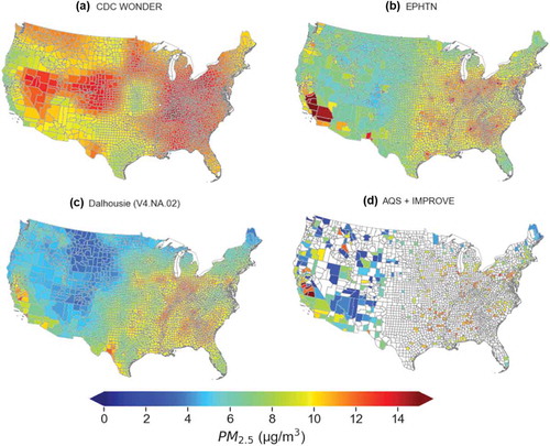
Figure 1b shows surface PM_2.5 from the CDC EPHTN, produced by the National Environmental Public Health Tracking Program in collaboration with EPA (EPHTP, also known as the Tracking Program), and based on Bayesian space-time downscaling (Berrocal, Gelfand, and Holland 2010a, 2010b, 2012). The EPHTN PM_2.5 data were previously used in epidemiology studies that track associations between PM_2.5 concentrations and a series of adverse health outcomes, including asthma-related emergency department visits, respiratory emergency department visits (Strosnider et al. 2019), exacerbation of existing asthma (MirabelMirabelli et al. 2016), cardiovascular chronic diseases (Weber et al. 2016), chronic kidney disease and end-stage renal disease (Bowe et al. 2018). In addition, the PM_2.5 estimates from EPHTN data were incorporated in a distributed lag nonlinear model when assessing the association between extreme heat and hospitalizations (Vaidyanathan et al. 2019). Although satellite data have not been incorporated into the EPHTN data, the Tracking Program partnered with NASA and Emory University to enhance spatial coverage of PM_2.5 in the southeast U.S. (Hu et al. 2014a), and evaluated various satellite-based data products for characterizing adverse health impacts resulting from wildfire smoke PM_2.5 (Gan et al. 2017). One feature of the EPHTN data is the relatively high concentrations in the western U.S. compared with the Dalhousie and AQS+IMPROVE fields in Figure 1. This difference is likely because EPHTN data used AQS monitors but not IMPROVE monitors in the fitting. PM_2.5 concentrations in the rural areas may be overestimated when rural, low-concentration measurements from the IMPROVE network are not used, and the predictions are based on interpolation of fits from AQS monitors in urban areas.

Figure 1c shows 2011 surface PM_2.5 fields from the Dalhousie data, which are based on models, satellites, and ground monitors. The data shown in Figure 1c are from V4.NA.02, and the data products are continually updated. van Donkelaar et al. (2010) describe the first global satellite-derived PM_2.5 dataset (V1.01), with subsequent datasets including additional satellite products (V2.01 (van Donkelaar et al. 2013)) and extending the time period of data availability (V3.01 (van Donkelaar et al. 2015)). The version shown in Figure 1c was developed for North America using AOD retrievals from multiple satellite products, combined with a GEOS-Chem simulation at 0.5°×0.67° resolution, and incorporation of local ground-based monitors through statistical fusion (V4.NA.02; (van Donkelaar et al. 2019)). This regional version builds upon updates made during development of the global product (V4.GL.02 (van Donkelaar et al. 2016)) that combine AOD from multiple satellite products based upon their relative uncertainties. The resultant 1-km PM_2.5 estimates are highly consistent (the spatial coefficient of determination (R²) = 0.81) with global out-of-sample cross-validated PM_2.5 concentrations from ground-based monitors. A variant of these data is also available (with similar performance) for the year 2014 (Shaddick et al. 2018b) as used in the GBD (Cohen et al. 2017). These datasets are currently being updated with newer satellite products, updated models, and new monitoring networks (Snider et al. 2015). The Dalhousie V4.NA.02 data for 2011 shown in Figure 1c capture the spatial gradients of the county-level monitoring data in Figure 1d. The Dalhousie data seem to show the best agreement with the AQS+IMPROVE data in the remote areas of the western U.S. and New England, which is consistent with another comparison study (Jin et al. 2019b). This feature indicates that incorporating satellite data can be valuable for improving estimation of PM_2.5 concentrations in remote areas where monitor coverage is sparse.

For comparison, Figure 1d shows a fusion of EPA AQS PM_2.5 and IMPROVE PM_2.5 allocated to the county scale (i.e., data within the same county are averaged to a single county-mean value). The two datasets were combined to provide a more comprehensive representation of both urban and rural areas in the United States. For EPA AQS PM_2.5, only counties with PM_2.5 concentrations collected over four complete quarters in 2011 were chosen, and averaged to estimate an annual value. For IMPROVE PM_2.5, monitor locations were matched with county Federal Information Processing Standards (FIPS) code and county-mean values were calculated. Then, the EPA AQS PM_2.5 and IMPROVE PM_2.5 were fused, that is, when both AQS and IMPROVE monitors occurred within a county, measurements from these two networks were averaged to derive the county mean. The agreement between the fused data fields (Figure 1a–c) with AQS-IMPROVE fused data (Figure 1d) may relate to the weight given to local data in the data fusion algorithm, and/or to the representativeness of a PM_2.5 monitor for a county average. Nevertheless, comparisons with observations can be useful for identifying differences among datasets based on quantitative evaluation metrics.

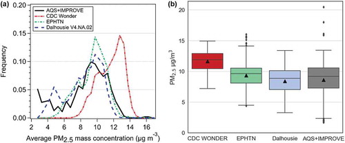
Figure 3a compares the frequency distributions of the three datasets with respect to the AQS-IMPROVE fused data. CDC WONDER consistently shows higher values than the other datasets. The Dalhousie dataset exhibits lower values of PM_2.5 overall with the widest frequency distribution (largest standard deviation in Figure 3b).

Results from our analyses of county-mean PM_2.5 estimates in 2011 are summarized in Table 2. The minimum annual county-level mass concentrations of PM_2.5 for CDC WONDER, EPHTN and Dalhousie are 7.2 μg/m³, 4.4 μg/m³ and 3.3 μg/m³, respectively, with the CDC WONDER’s minimum being the highest. Maximum values in each of the three datasets are similar (CDC WONDER: 14.9 μg/m³; EPHTN: 16 μg/m³; Dalhousie: 13.4 μg/m³). R² and the normalized mean bias based on standard formula (EPA 2018c) are calculated. Figure 2 shows the linear regression slope and intercept values. CDC WONDER exhibited the lowest R², 0.106, out of all the three datasets to averaged county-level AQS-IMPROVE fused data during a county-mean to county-mean comparison, and the highest normalized mean bias of 33.3%. But as for the grid-level validation, the validation of CDC WONDER’s surfacing algorithm showed an R² of 0.88 and RMSE of 1.6 μg/m³ for the Southeastern U.S., by comparing with EPA AQS monitors collocated with the grid cells of estimates (Al-Hamdan et al. 2009). CDC EPHTN demonstrated an R² of 0.649 and normalized mean bias of 12.2%. The Dalhousie dataset shows R² of 0.693 and normalized mean bias of 1.6% if the satellite-based data are sampled coincidentally at monitor locations from both the EPA AQS and IMPROVE networks before averaging by county and comparing, but degrades to an R² of 0.647 and normalized mean bias of −3.3% if county-level averages are taken before comparing with the in situ monitor data, and degrades still further to an R² of 0.527 and normalized mean bias of −9.2% if county-level averages are taken before comparing with the in situ monitor data and if the IMPROVE data are also excluded. The reduced agreement implies caution when using a limited number of primarily urban ground-based monitors to represent county averages, and motivates consideration of more spatially representative information such as from satellite and models as reviewed here. When further restricting the linear regression analyses to PM_2.5 < 15 μg m⁻³ only, the R² values for CDC WONDER and Dalhousie data only increase slightly, while the R² value for EPHTN remains the same.

Table 2. Summary of county-average 2011 annual mean PM_2.5 estimates of AQS+IMPROVE fused data, CDC WONDER, EPHTN and Dalhousie data in contiguous U.S.

PM2.5 data	AQS+IMPROVE	CDC WONDER	EPHTN	Dalhousie
Minimum PM2.5 value (μg/m^3)	1.7	7.2	4.4	3.3
Maximum PM2.5 value (μg/m^3)	20.4	14.9	16.0	13.4
R^2 *		0.106**	0.649	0.647
R^2 * for PM2.5 < 15 μg m^−3 only		0.136**	0.649	0.662
Normalized mean bias *		33.3%**	12.2%	−3.3%
Number of samples used in analysis	544	3102	3104	3104

Notes. *R² and normalized mean bias are calculated based on county-mean to county-mean comparison with respect to AQS+IMPROVE data of 2011 annual mean.

**This is based on county-mean to county-mean comparison, but as for the grid-level validation, the surfacing algorithm that was used to create the CDC WONDER dataset was also validated on the grid level for the Southeastern US that showed an R² of 0.88 and RMSE of 1.6 μg/m³ (Al-Hamdan et al. 2009).

Figure 2. Scatter plots of publicly available surface PM_2.5 datasets – (a) CDC WONDER, (b) EPHTN, and (c) Dalhousie (V4.NA.02) versus AQS+IMPROVE fused data. All data represent county-average 2011 annual mean. Two linear regressions are calculated: one for all data (top text box, red solid line showing this fit) and one for PM_2.5 < 15 μg m-3 only (bottom text box). Black solid line stands for 1:1 line. The value of a and b represent intercept and slope of the linear regression, respectively. The ±1σ stands for ± one standard deviation. The number of samples used for linear regression in (a), (b) and (c) are 543, 544 and 544, respectively.

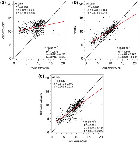
Figure 3. (a) Frequency distributions of the county-average 2011 annual mean PM_2.5 mass concentrations for the four data sets shown in Figure 1. (b) Mean (triangles), median (horizontal bar in the middle), 25 and 75 percentiles (bottom and top of the box, respectively) for the four data sets. Black dots represent outliers.

This comparison highlights the importance of methodology in estimating PM_2.5 surfaces. All three datasets used data from the EPA AQS; two used satellite AOD from the MODIS instrument; and two used advanced computer models. However, the results among these vary widely, and can be sensitive to assumptions about the spatial scale represented by individual PM_2.5 monitors. This comparison is limited to county averages of annual mean for 2011 and to only those counties with data availability over four complete quarters; so more extensive inter-comparison of PM_2.5 surfaces (including daily, grid-level and county-level comparisons for more counties and years) in future studies would provide helpful information to health and air quality organizations in selecting the appropriate data set for new applications.

PM_2.5 concentrations in global-scale estimates

The highest profile application of satellite-derived PM_2.5 fields has been the Global Burden of Diseases, Injuries, and Risk Factors Study (GBD). The GBD project continually evaluates PM_2.5 exposure using a consistent, globally applicable method representing the current state-of-the-science of data fusion of satellite, model, and monitor data.

For the 2010 GBD results reported in Lim et al. (2012), the PM_2.5 concentration estimates are described in Brauer et al. (2012) who used an average of satellite-derived PM_2.5 (van Donkelaar et al. 2010) and model (Van Dingenen et al. 2018) estimates that were recalibrated to align with in situ monitor data. For the 2013 GBD outcomes reported in Forouzanfar et al. (2015), PM_2.5 estimates from Brauer et al. (2016) were used that were based on a broader blend of satellites, a different modeling approach (Van Dingenen et al. 2018; van Donkelaar et al. 2015) and calibration against global monitoring data. More recently, the GBD 2015 results reported in Cohen et al. (2017) and Forouzanfar et al. (2016) used PM_2.5 concentrations estimated using significant methodological advances (Shaddick et al. 2018b; van Donkelaar et al. 2016). Rather than relying on a single global function to combine information from the different data sources (satellite-derived product, model, and in situ monitor data), a Bayesian hierarchical model was used to combine multiple streams of information with calibration coefficients defined at the country-specific scale (where possible). This allowed the final estimate to more heavily weigh the data source that yielded the most accurate PM_2.5 estimates (as evaluated through out-of-sample cross-validation) in different regions of the world.

The GBD 2016 results reported in Gakidou et al. (2017) continue to use a Bayesian hierarchical model to fuse geophysical satellite-derived PM_2.5 estimates (V4.GL.02.NoGWR (van Donkelaar et al. 2016)) with in situ PM_2.5 and PM₁₀ monitor data, using predictors, modeled aerosols from the global GEOS-Chem model, a factor related to elevation and urban proximity, and random effects and correlations across these terms (Shaddick et al. 2018a). Overall, the R² compared to out-of-sample cross-validation measurement increased from 0.64 to 0.91, and the root-mean-square error (RMSE) estimates reduced from 23 μg/m³ to 12 μg/m³, compared to GBD 2013 estimates (Shaddick et al. 2018a).

Besides differences of PM_2.5 estimates in different studies, the estimates of global exposure mortality can be affected by other factors such as causes of death being considered, regions being considered, and whether part of the PM_2.5 impact is being categorized as from indoor or outdoor PM_2.5 sources. For example, compared with the GBD studies, Burnett et al. (2018) used a different model – the Global Exposure Mortality Model (GEMM) to estimate association between outdoor PM_2.5 and non-accidental mortality, and predicted 8.9 million [95% confidence interval (CI): 7.5–10.3] deaths globally in 2015, which is 2.2 times of the prediction in the GBD (4.0 million; 95% CI: 3.3–4.8) (Forouzanfar et al. 2016).

Species and source-specific exposure estimates

Recently, an interest in identifying characteristics of PM_2.5 associated with health risks beyond total mass concentration has surged in the health and air quality fields, but progress is limited by robust evidence for the impact of PM_2.5 composition or emission sector on health outcomes (Kioumourtzoglou et al. 2015). A challenge in identifying such relationships has been the limited availability of species and source-specific exposure estimates. A review of Bates et al. (2019) summarized the recent progress for particle-bound reactive oxygen species (ROS) and oxidative potential (OP) measurement techniques. They discussed the compositional impacts on OP as well as health effects and highlighted the importance of specific emission sources including metals, organic carbon, vehicles, and biomass burning to OP. When there is a lack of measurements of OP at various times and locations, modeling approaches such as land-use regression and source impact regressions are often used (Bates et al. 2015; Fang et al. 2016; Yang et al. 2016). While models can be used to estimate species and sector-specific PM_2.5 exposures, model biases, limited resolution, and other uncertainties still limit the accuracy in model-based exposure estimates.

A number of different research groups have fused models with satellite and/or ground-based measurements, as discussed above. This same approach can be extended to the chemical speciation of aerosols available in models. For example, Ivey et al. (Ivey et al. 2015, 2017) used a combination of model sensitivity analysis and receptor modeling at monitor locations to estimate source contributions to total PM_2.5 from 20 different sources, including contributions from inorganic aerosol species and metals. Zhai et al. (2016) investigated mobile source contributions to air pollution concentration fields including PM_2.5 at 250-m fine resolution using a calibrated dispersion model and ground monitor data. Their results were applied to the estimation of prenatal exposure (Pennington et al. 2017) and childhood asthma outcomes (Pennington et al. 2018) due to traffic air pollution. Lee et al. (2015) used a combination of global adjoint sensitivity modeling and satellite-derived PM_2.5 concentrations to estimate the emitted species contributing to the global total premature deaths associated with long-term exposure to PM_2.5. Rundel et al. (2015) fused monitoring data and CMAQ output and provided summaries of five major PM_2.5 species for the continental U.S., including sulfate, nitrate, total carbonaceous matter, ammonium and fine soil/crustal material. Li et al. (2017) used a combination of global modeling (GEOS-Chem) and satellite-derived PM_2.5 concentrations to estimate trends in population-weighted speciated PM_2.5 concentrations worldwide. The species considered were sulfate, nitrate, ammonium, organic aerosol, black carbon, dust, and sea salt, and these were evaluated in comparison to speciated in situ ground monitor measurements in the U.S. The relative trends agreed to within a few percent in terms of the relative trends for most species, with the largest differences being those for natural components (sea salt and dust). Di, Koutrakis, and Schwartz (2016b) calibrated GEOS-chem model simulations using ground monitoring data and predicted 1 km × 1 km resolution PM_2.5 speciation data on daily basis in northeastern U.S. Additionally, van Donkelaar et al. (2019) directly extend the Dalhousie University satellite-derived PM_2.5 methodology to include estimates of chemical composition. Across all species, the agreement with speciated measurements in North America had an R² that ranged from 0.57 to 0.96, and a slope from 0.85 to 1.05, with generally the best agreement for sulfate, ammonium, and nitrate (R² between 0.86 and 0.96, slope between 0.99 and 1.01).

The upcoming MAIA (Multi-Angle Imager for Aerosols, preformulation ~2021) satellite-based remote sensing instrument will make radiometric and polarimetric measurements to better derive aerosol composition from space, helping to provide additional records of species and source-specific PM_2.5 to health researchers in several major urban areas worldwide (Diner et al. 2018).

Improved species and source-specific PM_2.5 surfaces will be of value for several reasons. For example, they can assist in the refinement of concentration-response relationships for epidemiological studies of the health impacts posed by particulate exposure. In addition, they can assist in identifying the PM_2.5 components or the emission sectors (e.g., transportation versus power generation) most responsible for PM_2.5’s toxicity.

Data assimilation and forecasting for episodic air pollution events

To date, most of the applications of data fusion among ground-based monitors, satellites, and/or model simulations were to support public health assessment retrospectively, since the measurements are only available for the past. To project future air quality, a conventional method is the “relative response factor” approach (EPA 2018d), which multiplies a base year’s fused concentration field by the ratio of the CMAQ model predictions between the future and base years. Such method has been applied to system development for meeting the NAAQS (Kelly et al. 2019) as well as impact analysis (EPA 2012). However, there is clear potential to extend data fusion approaches to air quality forecasting, using satellite and ground-based data as initial conditions assimilated into the models. Health-based PM forecasts tracking smoke from wildland fires are one example of the application of data assimilation.

Wildfires are becoming increasingly important sources for PM_2.5 pollution hazards due to the large quantity of emissions (Larkin, Raffuse, and Strand 2014), the acute episodic nature of the events, the difficulties associated with controlling them, and impacts of a changing climate (Spracklen et al. 2009). In particular, for the Northwest U.S., a positive trend was found in the 98th percentiles of PM_2.5 due to the increasing total areas burned by wildfires. This is in contrast to the decreasing trend of PM_2.5 in the other areas in the contiguous U.S. (McClure and Jaffe 2018). Several previous studies examined the adverse health effects from exposure to wildfire smoke in previous years based on observations and simulations. Rappold et al. (2017) used CMAQ model simulations with and without wildland and prescribed fires from 2008 to 2012 to quantify contribution of fire emissions to the ambient PM_2.5 levels. Their results showed that 30.5 million people in the U.S. lived in the areas where fire-emitted PM_2.5 is a large component of annual average value. Similarly, Fann et al. (2018) used CMAQ model simulations to assess the health impacts and economic value of wildland fire episodes in the U.S. from 2008 to 2012.

Compared with the retrospective analysis, the future-oriented forecasts for PM_2.5 emission from wildfire are even more challenging. Because of the episodic nature of wildfire emission, the forecasts would require daily or even hourly PM_2.5 estimates, rather than the annual exposure fields used in health studies like the GBD. In addition, fires typically occur in regions away from major cities where ground-based monitoring data are not always available, which imposes challenges on data assimilation.

There are multiple smoke forecasting systems in the U.S., all of which use models to provide future estimates of ground-level PM_2.5. Currently, satellite data are used in these systems to inform the location, timing, and characteristics of fire. Fire detection characteristics are combined with land cover data to calculate emissions into the model, and satellite AOD is used to evaluate model performance (Chen et al. 2008; Draxler and Hess 1998; Herron-Thorpe et al. 2012; Larkin et al. 2009; Schroeder et al. 2008; Stein et al. 2015; Vaughan et al. 2004).

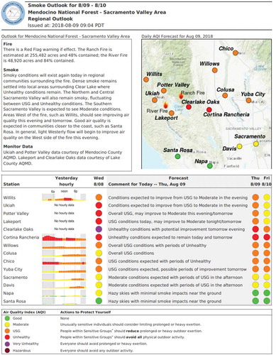
Among these smoke forecasting systems, the most direct integration of satellite AOD and wildland smoke prediction is performed by the Wildland Fire Air Quality Response Program (WFAQRP), which has been developed to address smoke issues from wildfires, bringing the latest in fire emissions and smoke transport science to Incident Management Teams, health and air quality agencies, and ultimately the public. This program provides smoke forecasting expertise, deploys temporary PM_2.5 monitors to augments existing monitoring systems, and communicates information on how to protect oneself from smoke. A daily Smoke Outlook is produced, forecasting expected smoke behavior and level of impact in the region of the fire (Figure 4). These smoke outlooks are initialized with a statistical model incorporating MODIS AOD and surface PM_2.5 monitoring data to forecast the AQI for the next day (Marsha and Larkin 2019).

Figure 4. An example of a smoke forecast issued for local communities by the Wildland Fire Air Quality Program. Example is from the river fire and ranch fire in the mendocino national forest issued for portions of Northern California and the Sacramento Valley area, California on August 9, 2018.

Discussion and conclusion

Remaining barriers for obtaining and applying PM_2.5 exposure for health applications

This review discusses the methods, sources, and application of spatially continuous PM_2.5 datasets derived from combinations of ground-based data, satellites, and/or atmospheric models. The data fusion products leverage the benefits of each data source, providing PM_2.5 exposure estimates over continuous spatial scales. This new resource for air quality data has already been used for health assessments, and has potential for application to research, public outreach, and environmental management. Nevertheless, several challenges remain in obtaining and applying PM_2.5 exposure for health applications. For example, missing data coverage in both ground monitors and satellite observations requires additional efforts for merging multiple data sources or interpolating data in space and time. When choosing the methods for data fusion or interpolation, users often need to weigh between the advantages and disadvantages of different methods. One may choose the efficient calculation of the Bayesian statistical downscaling method for lower spatial resolution (such as 12-km resolution in Wang et al. (2018)), while others may choose the more computational expensive methods that combine CTM, satellite and ground monitors (van Donkelaar et al. 2019), or machine learning techniques (Di et al. 2019; Hu et al. 2017; Reid et al. 2015). Methods that incorporate dispersion modeling may also be useful in some applications (Ahangar, Freedman, and Venkatram 2019; Scheffe et al. 2016). Depending on the methods being used in data fusion, assimilating the ground monitor data does not guarantee similar output of surface PM_2.5, as demonstrated in our case study of four datasets in Section 3.1. Such variability among publicly available datasets calls for more intercomparison studies to contrast and explain their differences. Future intercomparison studies are recommended to isolate individual factors contributing to comparison results, including but not limited to spatiotemporal variabilities of surface PM_2.5 (e.g., seasonal variability, topography, eastern versus western U.S.), data sources being used (model, satellite and/or monitors), regression of AOD – PM_2.5 relationships, representativeness of ground monitor data (e.g., weighting functions of monitors over a larger scale), spatial and temporal resolutions, etc. As end users of these PM_2.5 datasets, researchers in public health should be mindful that the agreement between fused PM_2.5 data and monitored PM_2.5 evaluated by R or R² are affected by multiple factors and assumptions being used in such evaluation (e.g., representativeness of monitor data, spatiotemporal interpolation, data resolutions, etc.). Varying sampling schedules for networks (i.e., higher frequency in urban areas versus lower frequency in rural areas) create another challenge when using ground monitor data as the gold standard, particularly for developing daily concentration fields. On days without rural sampling, predicted concentrations in rural areas might be overestimated because they are based on fits to predominantly urban monitoring. One way to combat this is to perform fusion on longer term monitor averages (monthly, quarterly, etc.). We recommend that researchers from both communities (i.e., data development and public health sectors) work together when applying the PM_2.5 estimates into health impacts assessments and/or air quality management actions. One example is to guide the model evaluations by the usage of PM_2.5 fields in health studies, which may be focused on a specific concentration range (e.g., lower concentrations in the rural areas versus higher concentrations in the urban areas), or a specific population. These specific targets may not be thoroughly tested by national or regional cross-validation.

Web-based tools for PM_2.5 exposure analyses

Despite the benefits of these data and the rapidly advancing research in this area, there are several key steps toward wider utilization of these data. One key step is to downsize spatially continuous data based on the types of applications. Although research groups may provide global or national data, most users require a small subset of data over a particular region and time period. Online mapping tools and options that allow users to subset data prior to download can significantly reduce the data management burden on users. Another key step is to maintain and foster training tutorials and seminars on specialized mapping software. For instance, the NASA Applied Remote Sensing Training (ARSET) program has been providing in-person and online tutorials for these purposes since 2009 (NASA 2019).

Several web-based tools are available for analyzing and predicting PM_2.5 exposure. The EPA Remote Sensing Information Gateway (RSIG), developed by U.S. EPA in collaboration with NASA, allows rapid retrieval and subsetting of satellite, model and ground-based data relevant to air quality. The RSIG website can be accessed at: https://www.epa.gov/hesc/remote-sensing-information-gateway, which provides multi-source, daily PM_2.5 data at up to 12-km horizontal resolution. Users can select only the subset of data needed for a particular application to be downloaded. RSIG can also combine multiple variables to simplify the burden of data analysis on the user. For example, if one is interested in comparing CMAQ-modeled PM_2.5 with AQS observations, the AQS observations can be subsetted and regridded to the model grid by specifying the model configuration (e.g., domain range, projection, resolution) (EPA RSIG 2019). As of April 2018, multiple PM_2.5 datasets are available from RSIG, including the EPA AQS in-situ monitor data, standard CMAQ model simulations over the continental U.S. conducted by the U.S. EPA, the FAQSD, and the combination of ground-based monitor and model data used by the CDC EPHTN. In addition, RSIG also provides up-to-date NASA MODIS AOD, and the National Environmental Satellite, Data and Information Service (NESDIS) Biomass Burning Emissions Data.

The University of California Berkeley’s Earth Air Quality Map (http://berkeleyearth.org/air-quality-real-time-map/) provides near-real-time maps of AQI values for PM_2.5 concentrations in the U.S. and several countries and regions outside of U.S. (e.g., China, Canada, Europe, etc.) at 0.1-degree resolution. As specified on the website, preliminary data from surface station measurements are being used with automated quality control procedure, and interpolated based on kriging method. Daily maps of PM_2.5 AQI values are available to download from June 2016 to March 2017.

When data are mapped through a web application, it can significantly reduce the burden of creating a map or plot. However, users often want the ability to create maps in a standard software platform to integrate with other aspects of their work. Currently, the netCDF is the most common format for atmospheric data, including PM_2.5 surfaces. Many programming languages, such as Python, the Interface Definition Language (IDL), MatLab, and the free National Center for Atmospheric Research (NCAR) Command Language (NCL) support netCDF data. ArcView GIS also supports netCDF, but users may have difficulty plotting large netCDF files in GIS. Because GIS platforms are so widely used among health, land planners, and policy communities, we recommend that data providers also include the standard release of GIS shapefiles as a distributed data format. Typically, shapefiles provide data in political or geographic spatial domains (e.g., U.S. counties or census tracts) rather than the grid format, which is typically used in atmospheric research.

Ongoing and future research efforts

Besides providing more guidance on the tools to potential users, improved utilization of PM_2.5 exposure datasets can be supported by increased validation. Because ground-based monitors, satellites, and models are often combined to estimated surface PM_2.5, there are few independent data sources for validation. A recent study over New York State uses independent ground-based observations from the New York City Community Air Quality Survey (NYCCAS) Program and the Saint Regis Mohawk Tribe Air Quality Program to evaluate seven PM_2.5 products (Jin et al. 2019b). Jin et al. suggest inclusion of satellite remote sensing improves the estimate of surface PM_2.5 in the remote area, but little gains over urban area. One of the networks with continuous efforts to evaluate satellite-derived PM_2.5 estimates is the publicly available Surface Particulate Matter Network SPARTAN (www.spartan-network.org) (Snider et al. 2015, 2016), which measures fine particle aerosol concentrations and composition continuously over multi-year periods at international sites where AOD is also measured by ground-based instruments. When validating PM_2.5 exposure data with ground-based observations, one caution is that the agreement between the fused data fields and in situ monitor data is related to the weight given to monitor data in the data fusion algorithm and the spatial and temporal scales that the in situ monitor data are assigned to represent. Certain criterion for data quality control may also cause a sampling bias.

Linking satellite observations of AOD with ground-level PM_2.5 estimates requires accurately understanding the relationship between aerosol extinction and aerosol mass abundance, which depends on multiple factors such as aerosol size distribution, hygroscopic growth (Brock et al. 2016a; Ziemba et al. 2013) and ambient relative humidity (Brock et al. 2016b). Targeted research efforts have been underway to advance understanding of these issues (Jin et al. 2019a). For example, the NASA DISCOVER-AQ aircraft campaign took place over four urban areas in the U.S. from 2011–2014, and provides extensive profiling of aerosol optical, chemical and microphysical properties at locations coincident with ground-based PM_2.5 sites. This multi-platform suite of observations is ideal for analyzing the relationship between satellite column AOD and ground-level PM_2.5 abundances (Crumeyrolle et al. 2014; Jin et al. 2019a).

While we have focused our discussion here on AOD, the most widely used metric for ambient particulates, there are other remote sensing instruments that can expand the value of satellite-based information (some of these are already in use in the data products presented here). For example, instruments aboard the Cloud-Aerosol Lidar and Infrared Pathfinder Satellite Observations (CALIPSO) provide vertical profiles of aerosol extinction with limited spatial coverage, which can be used to detect aerosols present above the surface (Ford and Heald 2013), and to correct model biases in the vertical profiles of aerosol extinction when quality-controlled retrievals are available (Geng et al. 2015; Li, Carlson, and Lacis 2015; van Donkelaar et al. 2016, 2013).

Ongoing research efforts have great potential to benefit spatially continuous PM_2.5 data fusion efforts. New geostationary satellites will provide improved temporal coverage, as they orbit with Earth, and can track the evolution of weather systems, wildfire smoke, urban pollution, and other factors affect ground-level PM_2.5. For example, the GOES-16 satellite provides AOD at a 2-km horizontal resolution every 5 min over the continental U.S. and other areas in its field of view. Improvements in these data, and other upcoming satellites, hold the potential to revolutionize the role of satellite data in estimating ground-level PM_2.5. Ongoing improvement in numerical modeling of the atmosphere, supported by decreasing computational cost, will also improve these data fusion products, allowing for higher-resolution model simulations. The rapid rise in low-cost PM monitors also offers opportunities for obtaining surface PM_2.5 information around the world, if low-cost monitors can be reliably calibrated.

Publicly available datasets are already supporting a wide range of air quality and health applications benefiting from spatially continuous PM_2.5 data. With the increased transparency of data products and methods, improved dissemination of data to support GIS mapping software, and plain-language communication of complex ideas have the potential to vastly expand the relevance of emerging data for health and air quality. As new users explore and evaluate these tools, their feedback to the research community can inform and improve future activities. A two-way dialog between researchers and stakeholders, e.g., the NASA Health and Air Quality Applied Sciences Team (HAQAST 2019) and the NASA ARSET training program (NASA 2019), can be very helpful in defining research priorities and ensuring outcomes to serve wider needs.

Acknowledgments

The following coauthors are members of the NASA Health and Air Quality Applied Sciences Team (HAQAST): M. Diao, T. Holloway, S. O’Neill, A. Fiore (NNX16AQ20G), and D. Henze. In addition, R.V. Martin, A. van Donkelaar, X. Jin, M.Z. Al-Hamdan, A. Vaidyanathan, P. Kinney, F. Freedman, and N. Larkin are HAQAST collaborators. M. Diao, F. Freedman, and M.Z. Al-Hamdan are funded by the NASA grant NNX16AQ91G. The CDC WONDER data were funded by the NASA Applied Sciences Health & Air Quality Program. The Dalhousie data are supported by the Atmospheric Composition Analysis Group at Dalhousie University in collaboration with scientists from NASA and the University of British Columbia. We appreciate technical guidance from the Wisconsin Department of Natural Resources in the interpretation and data selection for PM_2.5 in Figure 1d. The views expressed in this article are those of the authors and do not necessarily represent the views or policies of the Centers for Disease Control and Prevention, U.S. Environmental Protection Agency or other federal agencies involved in the study.

Additional information

Funding

This work was supported by the National Aeronautics and Space Administration [NNX16AQ91G, NNX16AQ92G, NNX16AQ20G, NNH16AD18I, NNX16AQ26G].

Notes on contributors

Minghui Diao

Minghui Diao is an assistant professor at San Jose State University. She received her B.S. degree from Peking University and Ph.D. degree from Princeton University. She is a member of the NASA Health and Air Quality Applied Sciences Team (HAQAST). Her current research interests include remote sensing of aerosol optical depth and PM2.5, and air quality assessment in California. For more information please see: www.cloud-research.org.

Tracey Holloway

Tracey Holloway is the Gaylord Nelson Distinguished Professor at the University of Wisconsin—Madison in the Nelson Institute for Environmental Studies and the Department of Atmospheric and Oceanic Sciences. She is the Team Lead for the NASA Health and Air Quality Applied Sciences Team. For more information see hollowaygroup.org and haqast.org.

Seohyun Choi

Seohyun Choi is a graduate student in Environment and Resources program at University of Wisconsin-Madison. She works with Dr. Tracey Holloway on NASA Health and Air Quality Applied Sciences Team to enhance the usage of air quality satellite data amongst public health organizations.

Susan M. O’Neill

Susan M. O’Neill is an Air Quality Scientist with the USDA Forest Service Pacific Northwest Research Station, AirFire Team, and has a Ph.D. from the Laboratory for Atmospheric Research at Washington State University. Her research interests include fire emissions calculation and atmospheric modeling of smoke plumes from prescribed fires and wildfires.

Mohammad Z. Al-Hamdan

Mohammad Z. Al-Hamdan is a Senior Research Scientist with the Universities Space Research Association at NASA Marshall Space Flight Center in Huntsville, Alabama, USA. He received his Ph.D. and M.S. degrees in Civil and Environmental Engineering from the University of Alabama in Huntsville. His research expertise includes remote sensing and GIS applications to environmental modeling and assessment for air quality, water, urban heat island, ecological and public health applications.

Aaron Van Donkelaar

Aaron van Donkelaar is a Research Associate in the Department of Physics and Atmospheric Science, Dalhousie University, and a Visiting Research Associate in the Department of Energy, Environmental & Chemical Engineering, Washington University in Saint Louis.

Randall V. Martin

Randall V. Martin is a Professor at Washington University, Professor and Arthur B. McDonald chair of research excellence at Dalhousie University, and a research associate at the Smithsonian Astrophysical Observatory. He serves as Co-Model Scientist for the GEOS-Chem model, on multiple satellite science teams, and as the principal investigator of the Surface Particulate Matter Network (SPARTAN).

Xiaomeng Jin

Xiaomeng Jin is a graduate student in Department of Earth and Environmental Sciences at Columbia University. She is working with Dr. Arlene Fiore working on atmospheric chemistry. Her research uses satellite observations and atmospheric chemistry models to analyze urban surface ozone and particulate matter pollution, and their sensitivities to precursor emissions.

Arlene M. Fiore

Arlene M. Fiore is a professor of atmospheric chemistry in the Department of Earth and Environmental Sciences of Lamont-Doherty Earth Observatory and Columbia University and an associate faculty member of the Earth Institute. For more information please see http://blog.ldeo.columbia.edu/atmoschem/.

Daven K. Henze

Daven K. Henze is an associate professor of mechanical engineering at the University of Colorado Boulder. He received his Ph.D. in chemical engineering from Caltech. He is a member of the NASA HAQAST team and researches the sources and fates of aerosols and trace-gases using adjoint sensitivity analysis, inverse modeling, and data assimilation.

Forrest Lacey

Forrest Lacey is an Advanced Study Program postdoc fellow at the National Center for Atmospheric Research. He also worked at the University of Colorado, Boulder as a postdoc and an adjunct professor.

Patrick L. Kinney

Patrick L. Kinney is a professor in the School of Public Health at Boston University. He received his B.S. degree in University of Colorado, Boulder, and his M.S. and ScD degrees from Harvard School of Public Health.

Frank Freedman

Frank Freedman is an adjunct faculty at San Jose State University. He received his B.S. and M.S. degrees from San Jose State University, and Ph.D. degree from Stanford University.

Narasimhan K. Larkin

Narasimhan K. Larkin is a research scientist and team leader with the USDA Forest Service Pacific Northwest Research Station’s AirFire Team and a member of the NASA HAQAST science team. He received his Ph.D. from the University of Washington studying climate variability. Since 2001 he has led research into wildfires, climate, and smoke, including developing emissions inventories, smoke forecasting systems, and operational decision support tools used across the United States and in other countries.

Yufei Zou

Yufei Zou is a postdoctoral research associate at Pacific Northwest National Laboratory (PNNL). Before joining PNNL, He received his Ph.D. degree in Earth and Atmospheric Sciences from Georgia Institute of Technology in 2017 and then worked at the University of Washington in Seattle for two years. His research mainly focuses on natural hazards and extreme weather events such as large wildfires and severe air pollution associated with global climate change.

James T. Kelly

James T. Kelly is an Environmental Scientist in the Office of Air Quality Planning & Standards at the U.S. Environmental Protection Agency.

Ambarish Vaidyanathan

Ambarish Vaidyanathan is a health scientist with the Centers for Disease Control and Prevention. He received his Masters and Doctoral degrees in Environmental Engineering from Georgia Institute of Technology, Atlanta, GA. Dr. Vaidyanathan has broad training and work experience in epidemiology, air quality modeling, statistics, and geographic information systems. He has collaborated with NASA and NASA funded partners on remote sensing projects since 2005.

References

- Ahangar, F. E., F. R. Freedman, and A. Venkatram. 2019. Using low-cost air quality sensor networks to improve the spatial and temporal resolution of concentration maps. Int. J. Environ. Res. Public Health 16 (7):1252. Multidisciplinary Digital Publishing Institute (MDPI). doi:10.3390/ijerph16071252.
- Al-Hamdan, A. Z., R. N. Albashaireh, M. Z. Al-Hamdan, and W. L. Crosson. 2017. The association of remotely sensed outdoor fine particulate matter with cancer incidence of respiratory system in the USA. J. Environ. Sci. Heal. Part A 52 (6) Taylor & Francis:547–54. doi:10.1080/10934529.2017.1284432.
- Al-Hamdan, A. Z., P. P. Preetha, R. N. Albashaireh, M. Z. Al-Hamdan, and W. L. Crosson. 2018b. Investigating the effects of environmental factors on autism spectrum disorder in the USA using remotely sensed data. Environ. Sci. Pollut. Res 25 (8) Springer Berlin Heidelberg:7924–36. doi:10.1007/s11356-017-1114-8.
- Al-Hamdan, A. Z., P. P. Preetha, M. Z. Al-Hamdan, W. L. Crosson, and R. N. Albashaireh. 2018a. Reconnoitering the linkage between cardiovascular disease mortality and long-term exposures to outdoor environmental factors in the USA using remotely-sensed data. J. Environ. Sci. Heal. Part A Taylor & Francis, 1–10. March. doi:10.1080/10934529.2018.1445083.
- Al-Hamdan, M. Z., W. L. Crosson, S. A. Economou, M. G. Estes, S. M. Estes, S. N. Hemmings, S. T. Kent, Puckett, M., Quattrochi, D.A., Rickman, D.L., Wade, G.M., and McClure, L.A. 2014. Environmental public health applications using remotely sensed data. Geocarto Int 29 (1) NIH Public Access: 85–98. doi: 10.1080/10106049.2012.715209
- Al-Hamdan, M. Z., W. L. Crosson, A. S. Limaye, D. L. Rickman, D. A. Quattrochi, M. G. Estes, J. R. Qualters, Sinclair, A.H., Tolsma, D.D., Adeniyi, K.A. and Niskar, A.S. 2009. Methods for characterizing fine particulate matter using ground observations and remotely sensed data: Potential use for environmental public health surveillance. J. Air Waste Manage. Assoc. 59 (7):865–81. doi:10.3155/1047-3289.59.7.865.
- Allen, G., C. Sioutas, P. Koutrakis, R. Reiss, F. W. Lurmann, and P. T. Roberts. 1997. Evaluation of the TEOM® method for measurement of ambient particulate mass in urban areas. J. Air Waste Manag. Assoc. 47 (6):682–89. doi:10.1080/10473289.1997.10463923.
- Anenberg, S. C., A. Belova, J. Brandt, N. Fann, S. Greco, S. Guttikunda, M. E. Heroux, Hurley, F., Krzyzanowski, M., Medina, S. and Miller, B. 2016. Survey of ambient air pollution health risk assessment tools. Risk Anal 36 (9):1718–36. doi:10.1111/risa.12540.
- Bates, J. T., R. J. Weber, J. Abrams, V. Verma, T. Fang, M. Klein, M. J. Strickland, Sarnat, S.E., Chang, H.H., Mulholland, J.A. and Tolbert, P.E. 2015. Reactive oxygen species generation linked to sources of atmospheric particulate matter and cardiorespiratory effects. Environ. Sci. Technol. 49 (22):13605–12. doi:10.1021/acs.est.5b02967.
- Bates, J. T., T. Fang, V. Verma, L. Zeng, R. J. Weber, P. E. Tolbert, J. Abrams, S. E. Sarnat, M. Klein, J. A. Mulholland, et al. 2019. Review of acellular assays of ambient particulate matter oxidative potential: Methods and relationships with composition, sources, and health effects. Environ. Sci. Technol. 53:4003–19. March. American Chemical Society, acs.est.8b03430. doi: 10.1021/acs.est.8b03430.
- Beckerman, B. S., M. Jerrett, M. Serre, R. V. Martin, S.-J. Lee, A. van Donkelaar, Z. Ross, J. Su, and R. T. Burnett. 2013. A hybrid approach to estimating national scale spatiotemporal variability of PM 2.5 in the contiguous United States. Environ. Sci. Technol 47 (13) American Chemical Society:7233–41. doi:10.1021/es400039u.
- Berrocal, V. J., A. E. Gelfand, and D. M. Holland. 2010a. A spatio-temporal downscaler for output from numerical models. J. Agric. Biol. Environ. Stat. 15 (2):176–97. doi:10.1007/s13253-009-0004-z.
- Berrocal, V. J., A. E. Gelfand, and D. M. Holland. 2010b. A bivariate space-time downscaler under space and time misalignment. Ann. Appl. Stat. 4 (4):1942–75. http://arxiv.org/abs/1004.1147.
- Berrocal, V. J., A. E. Gelfand, and D. M. Holland. 2012. Space-time data fusion under error in computer model output: An application to modeling air quality. Biometrics 68 (3):837–48. doi:10.1111/j.1541-0420.2011.01725.x.
- Bey, I., D. J. Jacob, R. M. Yantosca, J. A. Logan, B. D. Field, A. M. Fiore, Q. Li, H. Y. Liu, L. J. Mickley, and M. G. Schultz. 2001. Global modeling of tropospheric chemistry with assimilated meteorology: Model description and evaluation. J. Geophys. Res. Atmos 106 (D19) Wiley-Blackwell:23073–95. doi:10.1029/2001JD000807.
- Bi, J., J. H. Belle, Y. Wang, A. I. Lyapustin, A. Wildani, and Y. Liu. 2019. Impacts of snow and cloud covers on satellite-derived PM2.5 levels. Remote Sens. Environ 221 (February) Elsevier:665–74. doi:10.1016/J.RSE.2018.12.002.
- Bowe, B., Y. Xie, T. Li, Y. Yan, H. Xian, and Z. Al-Aly. 2018. Particulate matter air pollution and the risk of incident CKD and progression to ESRD. J. Am. Soc. Nephrol 29 (1) American Society of Nephrology:218–30. doi:10.1681/ASN.2017030253.
- Brauer, M., M. Amann, R. T. Burnett, A. Cohen, F. Dentener, M. Ezzati, S. B. Henderson, Krzyzanowski, M., Martin, R.V., Van Dingenen, R. and Van Donkelaar, A. 2012. Exposure assessment for estimation of the global burden of disease attributable to outdoor air pollution. Environ. Sci. Technol 46 (2):652–60. doi:10.1021/es2025752.
- Brauer, M., G. Freedman, J. Frostad, A. van Donkelaar, R. V. Martin, F. Dentener, R. van Dingenen, Estep, K., Amini, H., Apte, J.S. and Balakrishnan, K. 2016. Ambient air pollution exposure estimation for the global burden of disease 2013. Environ. Sci. Technol 50 (1):79–88. doi:10.1021/acs.est.5b03709.
- Brock, C. A., N. L. Wagner, B. E. Anderson, A. R. Attwood, A. Beyersdorf, P. Campuzano-Jost, A. G. Carlton, Day, D.A., Diskin, G.S., Gordon, T.D. and Jimenez, J.L. 2016a. Aerosol optical properties in the Southeastern United States in summer - part 1: Hygroscopic growth. Atmos. Chem. Phys. 16 (8):4987–5007. doi:10.5194/acp-16-4987-2016.
- Brock, C. A., N. L. Wagner, B. E. Anderson, A. Beyersdorf, P. Campuzano-Jost, D. A. Day, G. S. Diskin, Gordon, T.D., Jimenez, J.L., Lack, D.A. and Liao, J. 2016b. Aerosol optical properties in the Southeastern United States in summer - part 2: Sensitivity of aerosol optical depth to relative humidity and aerosol parameters. Atmos. Chem. Phys 16 (8):5009–19. doi:10.5194/acp-16-5009-2016.
- Brook, R. D., S. Rajagopalan, C. A. Pope, J. R. Brook, A. Bhatnagar, A. V. Diez-Roux, F. Holguin, Hong, Y., Luepker, R.V., Mittleman, M.A. and Peters, A. 2010. Particulate matter air pollution and cardiovascular disease: An update to the scientific statement from the American heart association. Circulation 121 (21):2331–78. doi:10.1161/CIR.0b013e3181dbece1.
- Buchard, V., C. A. Randles, A. M. Da Silva, A. Darmenov, P. R. Colarco, R. Govindaraju, R. Ferrare, Hair, J., Beyersdorf, A.J., Ziemba, L.D. and Yu, H. 2017. The MERRA-2 aerosol reanalysis, 1980 onward. Part II: Evaluation and case studies. J. Clim. 30 (17):6851–72. doi:10.1175/JCLI-D-16-0613.1.
- Burnett, R., H. Chen, M. Szyszkowicz, N. Fann, B. Hubbell, C. A. Pope, J. S. Apte, Brauer, M., Cohen, A., Weichenthal, S. and Coggins, J. 2018. Global estimates of mortality associated with long-term exposure to outdoor fine particulate matter. Proc. Natl. Acad. Sci. USA 115 (38) National Academy of Sciences:9592–97. doi:10.1073/pnas.1803222115.
- Centers for Disease Control and Prevention. 2018. Home - CDC tracking network. https://ephtracking.cdc.gov/showHome.
- Chen, J., J. Vaughan, J. Avise, S. O’Neill, and B. Lamb. 2008. Enhancement and evaluation of the AIRPACT ozone and PM2.5 forecast system for the Pacific Northwest. J. Geophys. Res. Atmos. 113 (14):1–20. doi:10.1029/2007JD009554.
- Chow, J. C., P. Doraiswamy, J. G. Watson, L.-W. A. Chen, S. S. H. Ho, and D. A. Sodeman. 2008. Advances in integrated and continuous measurements for particle mass and chemical composition. J. Air Waste Manage. Assoc 58 (2) Taylor & Francis Group:141–63. doi:10.3155/1047-3289.58.2.141.
- Chow, J. C., and J. G. Watson. 1998. Guideline on speciated particulate monitoring. https://www3.epa.gov/ttnamti1/files/ambient/pm25/spec/drispec.pdf.
- Chu, Y., Y. Liu, X. Li, Z. Liu, H. Lu, Y. Lu, Z. Mao, X. Chen, N. Li, M. Ren, et al. 2016. A review on predicting ground PM2.5 concentration using satellite aerosol optical depth. Atmosphere (Basel) 7 (10) Multidisciplinary Digital Publishing Institute:129. doi:10.3390/atmos7100129.
- Cohen, A. J., M. Brauer, R. Burnett, H. R. Anderson, J. Frostad, K. Estep, K. Balakrishnan, Brunekreef, B., Dandona, L., Dandona, R. and Feigin, V. 2017. Estimates and 25-year trends of the global burden of disease attributable to ambient air pollution: An analysis of data from the global burden of diseases study 2015. Lancet 389 (10082) The Author(s). Published by Elsevier Ltd. This is an Open Access article under the CC BY 4.0 license:1907–18. doi:10.1016/S0140-6736(17)30505-6.
- Crumeyrolle, S., G. Chen, L. Ziemba, A. Beyersdorf, L. Thornhill, E. Winstead, R. H. Moore, M. A. Shook, C. Hudgins, and B. E. Anderson. 2014. Factors that influence surface PM2.5 values inferred from satellite observations: Perspective gained for the US Baltimore-Washington Metropolitan Area during DISCOVER-AQ. Atmos. Chem. Phys. 14 (4):2139–53. doi:10.5194/acp-14-2139-2014.
- Di, Q., H. Amini, L. Shi, I. Kloog, R. Silvern, J. Kelly, M. B. Sabath, C. Choirat, P. Koutrakis, A. Lyapustin, et al. 2019. An ensemble-based model of PM2.5 concentration across the contiguous United States with high spatiotemporal resolution. Environment International 130 (September) Pergamon:104909. doi:10.1016/J.ENVINT.2019.104909.
- Di, Q., I. Kloog, P. Koutrakis, A. Lyapustin, Y. Wang, and J. Schwartz. 2016a. Assessing PM2.5 exposures with high spatiotemporal resolution across the continental United States. Environ. Sci. Technol 50 (9) American Chemical Society:4712–21. doi:10.1021/acs.est.5b06121.
- Di, Q., P. Koutrakis, and J. Schwartz. 2016b. A hybrid prediction model for PM2.5 mass and components using a chemical transport model and land use regression. Atmos. Environ 131 (April) Pergamon:390–99. doi:10.1016/J.ATMOSENV.2016.02.002.
- Diner, D. J., S. W. Boland, M. Brauer, C. Bruegge, K. A. Burke, R. Chipman, L. Di Girolamo, M. J. Garay, S. Hasheminassab, and E. Hyer. 2018. Advances in multiangle satellite remote sensing of speciated airborne particulate matter and association with adverse health effects: From MISR to MAIA. J. Appl. Remote Sens 12 (04) International Society for Optics and Photonics:1. doi:10.1117/1.JRS.12.042603.
- Dominici, F., R. D. Peng, M. L. Bell, L. Pham, A. McDermott, S. L. Zeger, and J. M. Samet. 2006. Fine particulate air pollution and hospital admission for cardiovascular and respiratory diseases. JAMA 295 (10):1127–34. doi:10.1001/jama.295.10.1127.
- Draxler, R. R., and G. D. Hess. 1998. An overview of the HYSPLIT_4 modelling system for trajectories, dispersion and deposition. Aust. Meteorol. Mag. 47 (4):295–308.
- Engel-Cox, J. A., C. H. Holloman, B. W. Coutant, and R. M. Hoff. 2004. Qualitative and quantitative evaluation of MODIS satellite sensor data for regional and urban scale air quality. Atmos. Environ. 38 (16):2495–509. doi:10.1016/j.atmosenv.2004.01.039.
- EPA. 2012. Regulatory impact analysis for the final revisions to the national ambient air quality standards for particulate matter. Research Triangle Park, NC: Office of Air Quality Planning and Standards. https://www3.epa.gov/ttn/ecas/regdata/RIAs/finalria.pdf.
- EPA. 2016. Technical information about fused air quality surface using downscaling tool: Metadata description. https://www.epa.gov/sites/production/files/2016-07/documents/data_fusion_meta_file_july_2016.pdf.
- EPA. 2017. Profile of version 1 of the 2014 national emissions inventory. Accessed April 27, 2018. https://www.epa.gov/sites/production/files/2017-04/documents/2014neiv1_profile_final_april182017.pdf.
- EPA. 2018a. Health and environmental effects of Particulate Matter (PM). Accessed April 27, 2018. https://www.epa.gov/pm-pollution/particulate-matter-pm-basics#PM.
- EPA. 2018b. EPA airdata air quality monitors. Accessed March 10, 2019. https://www.epa.gov/outdoor-air-quality-data.
- EPA. 2018c. Air quality modeling technical support document for the updated 2023 projected ozone design values. https://www.epa.gov/sites/production/files/2018-06/documents/aq_modelingtsd_updated_2023_modeling_o3_dvs.pdf.
- EPA. 2018d. Modeling guidance for demonstrating attainment of air quality goals for ozone, PM2.5, and regional haze. Research Triangle Park, NC. https://www3.epa.gov/ttn/scram/guidance/guide/O3-PM-RH-Modeling_Guidance-2018.pdf.
- EPA RSIG. 2019. Accessed March 10, 2019. https://www.epa.gov/hesc/remote-sensing-information-gateway.
- European Committee for Standardization (CEN). 1998. Standard EN 12341. Air quality – determination of the PM10 fraction of suspended particulate matter – reference method and field test procedure to demonstrate reference equivalence of measurement methods. European Standard EN 12341.
- Fang, T., V. Verma, J. T. Bates, J. Abrams, M. Klein, M. J. Strickland, S. E. Sarnat, H. H. Chang, J. A. Mulholland, P. E. Tolbert, et al. 2016. Oxidative potential of ambient water-soluble PM2.5 in the southeastern United States: Contrasts in sources and health associations between ascorbic acid (AA) and dithiothreitol (DTT) assays. Atmos. Chem. Phys. 16 (6):3865–79. doi:10.5194/acp-16-3865-2016.
- Fann, N., B. Alman, R. A. Broome, G. G. Morgan, F. H. Johnston, G. Pouliot, and A. G. Rappold. 2018. The health impacts and economic value of wildland fire episodes in the U.S.: 2008–2012. Sci. Total Environ 610–611 (January) Elsevier:802–09. doi:10.1016/J.SCITOTENV.2017.08.024.
- Ford, B., and C. L. Heald. 2013. Aerosol loading in the Southeastern United States: Reconciling surface and satellite observations. Atmos. Chem. Phys. 13 (18):9269–83. doi:10.5194/acp-13-9269-2013.
- Ford, B., and C. L. Heald. 2016. Exploring the uncertainty associated with satellite-based estimates of premature mortality due to exposure to fine particulate matter. Atmos. Chem. Phys. 16 (5):3499–523. doi:10.5194/acp-16-3499-2016.
- Forouzanfar, M. H., A. Afshin, L. T. Alexander, H. R. Anderson, Z. A. Bhutta, S. Biryukov, M. Brauer, Burnett, R., Casey, D., Coates, M.M. and Cohen, A. 2016. Global, regional, and national comparative risk assessment of 79 behavioural, environmental and occupational, and metabolic risks or clusters of risks, 1990–2015: A systematic analysis for the global burden of disease study 2015. Lancet 388 (10053):1659–724. doi:10.1016/S0140-6736(16)31679-8.
- Forouzanfar, M. H., L. Alexander, H. R. Anderson, V. F. Bachman, S. Biryukov, M. Brauer, R. Burnett, Cercy, K., Charlson, F.J. and Cohen, A.J. 2015. Global, regional, and national comparative risk assessment of 79 behavioural, environmental and occupational, and metabolic risks or clusters of risks in 188 countries, 1990–2013: A systematic analysis for the global burden of disease study 2013. Lancet 386 (10010) Elsevier:2287–323. doi:10.1016/S0140-6736(15)00128-2.
- Friberg, M. D., R. A. Kahn, H. A. Holmes, H. H. Chang, S. E. Sarnat, P. E. Tolbert, A. G. Russell, and J. A. Mulholland. 2017. Daily ambient air pollution metrics for five cities: Evaluation of data-fusion-based estimates and uncertainties. Atmos. Environ 158 (2) Elsevier Ltd:36–50. doi:10.1016/j.atmosenv.2017.03.022.
- Friberg, M. D., X. Zhai, H. A. Holmes, H. H. Chang, M. J. Strickland, S. E. Sarnat, P. E. Tolbert, A. G. Russell, and J. A. Mulholland. 2016. Method for fusing observational data and chemical transport model simulations to estimate spatiotemporally resolved ambient air pollution. Environ. Sci. Technol 50 (7) American Chemical Society:3695–705. doi:10.1021/acs.est.5b05134.
- Gakidou, E., A. Afshin, A. A. Abajobir, K. H. Abate, C. Abbafati, K. M. Abbas, F. Abd-Allah, Abdulle, A.M., Abera, S.F., Aboyans, V. and Abu-Raddad, L.J. 2017. Global, regional, and national comparative risk assessment of 84 behavioural, environmental and occupational, and metabolic risks or clusters of risks, 1990-2016: A systematic analysis for the global burden of disease study 2016. Lancet (London, England) 390 (10100) Elsevier:1345–422. doi:10.1016/S0140-6736(17)32366-8.
- Gan, R. W., B. Ford, W. Lassman, G. Pfister, A. Vaidyanathan, E. Fischer, J. Volckens, J. R. Pierce, and S. Magzamen. 2017. Comparison of wildfire smoke estimation methods and associations with cardiopulmonary-related hospital admissions. GeoHealth 1 (3) John Wiley & Sons, Ltd:122–36. doi:10.1002/2017GH000073.
- Geng, G., Q. Zhang, R. V. Martin, A. van Donkelaar, H. Huo, H. Che, J. Lin, and K. He. 2015. Estimating long-term PM2.5 concentrations in China using satellite-based aerosol optical depth and a chemical transport model. Remote Sens. Environ 166 Elsevier Inc.:262–70. doi:10.1016/j.rse.2015.05.016.
- Gupta, P., and S. A. Christopher. 2009. Particulate matter air quality assessment using integrated surface, satellite, and meteorological products: 2. a neural network approach. J. Geophys. Res. Atmos. 114 (20):1–14. doi:10.1029/2008JD011497.
- Gupta, P., S. A. Christopher, J. Wang, R. Gehrig, Y. Lee, and N. Kumar. 2006. Satellite remote sensing of particulate matter and air quality assessment over global cities. Atmos. Environ. 40 (30):5880–92. doi:10.1016/j.atmosenv.2006.03.016.
- Haikerwal, A., M. Akram, A. Del Monaco, K. Smith, M. R. Sim, M. Meyer, A. M. Tonkin, M. J. Abramson, and M. Dennekamp. 2015. Impact of fine Particulate Matter (PM2.5) exposure during wildfires on cardiovascular health outcomes. J. Am. Heart Assoc. 4 (7):1–10. doi:10.1161/JAHA.114.001653.
- HAQAST, N. 2019. NASA HEALTH AND AIR QUALITY APPLIED SCIENCES TEAM. Accessed March 10, 2019. https://haqast.org/.
- Henderson, S. B., and F. H. Johnston. 2012. Measures of forest fire smoke exposure and their associations with respiratory health outcomes. Curr. Opin. Allergy Clin. Immunol. 12 (3):221–27. doi:10.1097/ACI.0b013e328353351f.
- Hering, S., and G. Cass. 1999. The magnitude of bias in the measurement of PM2.5 arising from volatilization of particulate nitrate from teflon filters. J. Air Waste Manag. Assoc. 49 (6):725–33. doi:10.1080/10473289.1999.10463843.
- Herron-Thorpe, F. L., G. H. Mount, L. K. Emmons, B. K. Lamb, S. H. Chung, and J. K. Vaughan. 2012. Regional air-quality forecasting for the Pacific Northwest using MOPITT/TERRA assimilated carbon monoxide MOZART-4 forecasts as a near real-time boundary condition. Atmos. Chem. Phys. 12 (12):5603–15. doi:10.5194/acp-12-5603-2012.
- Hoek, G., R. M. Krishnan, R. Beelen, A. Peters, B. Ostro, B. Brunekreef, and J. D. Kaufman. 2013. Long-term air pollution exposure and cardio- respiratory mortality: A review. Environ. Heal. 12 (1):43. doi:10.1186/1476-069X-12-43.
- Hoff, R. M., and S. A. Christopher. 2009. Remote sensing of particulate pollution from space: Have we reached the promised land? J. Air Waste Manage. Assoc 59 (6) Taylor & Francis Group:645–75. doi:10.3155/1047-3289.59.6.645.
- Hu, X., J. H. Belle, X. Meng, A. Wildani, L. A. Waller, M. J. Strickland, and Y. Liu. 2017. Estimating PM 2.5 concentrations in the conterminous United States using the random forest approach. Environ. Sci. Technol 51 (12) American Chemical Society:6936–44. doi:10.1021/acs.est.7b01210.
- Hu, X., L. A. Waller, A. Lyapustin, Y. Wang, M. Z. Al-Hamdan, W. L. Crosson, M. G. Estes, S. M. Estes, D. A. Quattrochi, S. J. Puttaswamy, et al. 2014a. Estimating ground-level PM2.5 concentrations in the Southeastern United States using MAIAC AOD retrievals and a two-stage model. Remote Sens. Environ 140 (2014) Elsevier Inc.:220–32. doi:10.1016/j.rse.2013.08.032.
- Hu, X., L. A. Waller, A. Lyapustin, Y. Wang, and Y. Liu. 2014b. 10-year spatial and temporal trends of PM2.5 concentrations in the Southeastern US estimated using high-resolution satellite data. Atmos. Chem. Phys. 14 (12):6301–14. doi:10.5194/acp-14-6301-2014.
- Huang, R., X. Zhai, C. E. Ivey, M. D. Friberg, X. Hu, Y. Liu, Q. Di, J. Schwartz, J. A. Mulholland, and A. G. Russell. 2018. Air pollutant exposure field modeling using air quality model-data fusion methods and comparison with satellite AOD-derived fields: Application over North Carolina, USA. Air Qual. Atmos. Heal. 11 (1):11–22. doi:10.1007/s11869-017-0511-y.
- Huijnen, V., J. Williams, M. van Weele, T. van Noije, M. Krol, F. Dentener, A. Segers, S. Houweling, W. Peters, J. de Laat, et al. 2010. The global chemistry transport model TM5: Description and evaluation of the tropospheric chemistry version 3.0. Geosci. Model Dev. 3 (2):445–73. doi:10.5194/gmd-3-445-2010.
- Ivey, C., H. Holmes, G. Shi, S. Balachandran, Y. Hu, and A. G. Russell. 2017. Development of PM 2.5 source profiles using a hybrid chemical transport-receptor modeling approach. Environ. Sci. Technol 51 (23) American Chemical Society:13788–96. doi:10.1021/acs.est.7b03781.
- Ivey, C. E., H. A. Holmes, Y. T. Hu, J. A. Mulholland, and A. G. Russell. 2015. Development of PM2.5 source impact spatial fields using a hybrid source apportionment air quality model. Geosci. Model Dev. 8 (7):2153–65. doi:10.5194/gmd-8-2153-2015.
- Jin, X., A. M. Fiore, K. Civerolo, J. Bi, Y. Liu, A. Van Donkelaar, R. Martin, M. Al-Hamdan, Y. Zhang, T. Z. Insaf, et al. 2019b. Comparison of multiple PM2.5 exposure products for estimating health benefits of emission controls over New York State, USA. Environ. Res. Lett 14:084023. June. IOP Publishing. doi:10.1088/1748-9326/ab2dcb.
- Jin, X., A. M. Fiore, G. Curci, A. Lyapustin, K. Civerolo, M. Ku, A. van Donkelaar, and R. V. Martin. 2019a. Assessing uncertainties of a geophysical approach to estimate surface fine particulate matter distributions from satellite-observed aerosol optical depth. Atmos. Chem. Phys. 19 (1):295–313. doi:10.5194/acp-19-295-2019.
- Keller, J. P., and R. D. Peng. 2019. Error in estimating area‐level air pollution exposures for epidemiology. Environmetrics John Wiley & Sons, Ltd. e2573. May. doi:10.1002/env.2573.
- Kelly, J. T., C. J. Jang, B. Timin, B. Gantt, A. Reff, Y. Zhu, S. Long, and A. Hanna. 2019. A system for developing and projecting PM2.5 spatial fields to correspond to just meeting national ambient air quality standards. Atmos. Environ X 2 (April) Elsevier:100019. doi:10.1016/J.AEAOA.2019.100019.
- Kim, Y. H., S. H. Warren, Q. T. Krantz, C. King, R. Jaskot, W. T. Preston, B. J. George, Hays, M.D., Landis, M.S., Higuchi, M. and DeMarini, D.M. 2018. Mutagenicity and lung toxicity of smoldering vs. flaming emissions from various biomass fuels: Implications for health effects from wildland fires. Environ. Health Perspect. 126 (01):017011. doi:10.1289/EHP2200.
- Kioumourtzoglou, M.-A., E. Austin, P. Koutrakis, F. Dominici, J. Schwartz, and A. Zanobetti. 2015. PM2.5 and survival among older adults: Effect modification by particulate composition. HHS Public Access 26 (3):321–27. doi:10.1097/EDE.0000000000000269.
- Klimont, Z., K. Kupiainen, C. Heyes, P. Purohit, J. Cofala, P. Rafaj, J. Borken-Kleefeld, and W. Schöpp. 2017. Supplement of global anthropogenic emissions of particulate matter including black carbon. Atmos. Chem. Phys. 17 (14):8681–723. doi:10.5194/acp-17-8681-2017.
- Kloog, I., A. A. Chudnovsky, A. C. Just, F. Nordio, P. Koutrakis, B. A. Coull, A. Lyapustin, Y. Wang, and J. Schwartz. 2014. A new hybrid spatio-temporal model for estimating daily multi-year PM2.5 concentrations across Northeastern USA using high resolution aerosol optical depth data. Atmos. Environ. 95:581–90. doi:10.1016/j.atmosenv.2014.07.014.
- Koelemeijer, R. B. A., C. D. Homan, and J. Matthijsen. 2006. Comparison of spatial and temporal variations of aerosol optical thickness and particulate matter over Europe. Atmos. Environ. 40 (27):5304–15. doi:10.1016/j.atmosenv.2006.04.044.
- Kokhanovsky, A. A., F.-M. Breon, A. Cacciari, E. Carboni, D. Diner, W. Di Nicolantonio, R. G. Grainger, W. M. F. Grey, R. Höller, K.-H. Lee, et al. 2007. Aerosol remote sensing over land: A comparison of satellite retrievals using different algorithms and instruments. Atmos. Res 85 (3–4) Elsevier:372–94. doi:10.1016/J.ATMOSRES.2007.02.008.
- Krewski, D., M. Jerrett, R. T. Burnett, R. Ma, E. Hughes, Y. Shi, M. C. Turner, Pope, C.A. III, Thurston, G., Calle, E.E. and Thun, M.J. 2009. Extended follow-up and spatial analysis of the American cancer society study linking particulate air pollution and mortality. Res. Rep. Health. Eff. Inst 140 (May):5–114; discussion 115-36. http://www.ncbi.nlm.nih.gov/pubmed/19627030.
- Laden, F., L. M. Neas, D. W. Dockery, and J. Schwartz. 2000. Association of fine particulate matter from different sources with daily mortality in six U.S. cities. Environ. Health Perspect 108 (10) National Institute of Environmental Health Science:941–47. doi:10.1289/ehp.00108941.
- Larkin, N. K., S. M. O’Neill, R. Solomon, S. Raffuse, T. Strand, D. C. Sullivan, C. Krull, M. Rorig, J. Peterson, and S. A. Ferguson. 2009. The bluesky smoke modeling framework. Int. J. Wildl. Fire 18 (8):906–20. doi:10.1071/WF07086.
- Larkin, N. K., S. M. Raffuse, and T. M. Strand. 2014. Wildland fire emissions, carbon, and climate: U.S. emissions inventories. For. Ecol. Manage 317 Elsevier B.V.:61–69. doi:10.1016/j.foreco.2013.09.012.
- Lassman, W., B. Ford, R. W. Gan, G. Pfister, S. Magzamen, E. V. Fischer, and J. R. Pierce. 2017. Spatial and temporal estimates of population exposure to wildfire smoke during the Washington state 2012 wildfire season using blended model, satellite, and in situ data. GeoHealth 1 (3) Wiley-Blackwell:106–21. doi:10.1002/2017GH000049.
- Lee, C. J., R. V. Martin, D. K. Henze, M. Brauer, A. Cohen, and A. van Donkelaar. 2015. Response of global particulate-matter-related mortality to changes in local precursor emissions. Environ. Sci. Technol. 49 (7):4335–44. doi:10.1021/acs.est.5b00873.
- Lee, M., I. Kloog, A. Chudnovsky, A. Lyapustin, Y. Wang, S. Melly, B. Coull, P. Koutrakis, and J. Schwartz. 2016. Spatiotemporal prediction of fine particulate matter using high-resolution satellite images in the Southeastern US 2003-2011. J. Expo. Sci. Environ. Epidemiol 26 (4) NIH Public Access:377–84. doi:10.1038/JES.2015.41.
- Lennartson, E. M., J. Wang, J. Gu, L. Castro Garcia, C. Ge, M. Gao, M. Choi, P. E. Saide, G. R. Carmichael, J. Kim, et al. 2018. Diurnal variation of aerosol optical depth and PM2.5 in South Korea: A synthesis from AERONET, satellite (GOCI), KORUS-AQ observation, and the WRF-chem model. Atmos. Chem. Phys. 18 (20):15125–44. doi:10.5194/acp-18-15125-2018.
- Li, C., R. V. Martin, B. L. Boys, A. van Donkelaar, and S. Ruzzante. 2016. Evaluation and application of multi-decadal visibility data for trend analysis of atmospheric haze. Atmos. Chem. Phys. 16 (4):2435–57. doi:10.5194/acp-16-2435-2016.
- Li, C., R. V. Martin, A. van Donkelaar, B. L. Boys, M. S. Hammer, J. W. Xu, E. A. Marais, A. Reff, M. Strum, D. A. Ridley, et al. 2017. Trends in chemical composition of global and regional population-weighted fine particulate matter estimated for 25 years. Environ. Sci. Technol. 51 (19):11185–95. doi:10.1021/acs.est.7b02530.
- Li, J., B. E. Carlson, and A. A. Lacis. 2015. How well do satellite AOD observations represent the spatial and temporal variability of PM2.5 concentration for the United States? Atmos. Environ 102 (February) Pergamon:260–73. doi:10.1016/J.ATMOSENV.2014.12.010.
- Lim, S. S., T. Vos, A. D. Flaxman, G. Danaei, K. Shibuya, H. Adair-Rohani, M. A. AlMazroa, Amann, M., Anderson, H.R., Andrews, K.G. and Aryee, M. 2012. A comparative risk assessment of burden of disease and injury attributable to 67 risk factors and risk factor clusters in 21 regions, 1990–2010: A systematic analysis for the global burden of disease study 2010. Lancet 380 (9859):2224–60. doi:10.1016/S0140-6736(12)61766-8.
- Lin, H., Y. Guo, Q. Di, Y. Zheng, P. Kowal, J. Xiao, T. Liu, Li, X., Zeng, W., Howard, S.W. and Nelson, E.J. 2017. Ambient PM 2.5 and stroke. Stroke 48 (5):1191–97. doi:10.1161/STROKEAHA.116.015739.
- Liu, J. C., G. Pereira, S. A. Uhl, M. A. Bravo, and M. L. Bell. 2015. A systematic review of the physical health impacts from non-occupational exposure to wildfire smoke. Environ. Res. 136 (January):120–32. doi:10.1016/j.envres.2014.10.015.
- Liu, Y., M. Franklin, R. Kahn, and P. Koutrakis. 2007. Using aerosol optical thickness to predict ground-level PM2.5 concentrations in the St. Louis Area: A comparison between MISR and MODIS. Remote Sens. Environ. 107 (1–2):33–44. doi:10.1016/j.rse.2006.05.022.
- Liu, Y., C. J. Paciorek, and P. Koutrakis. 2009. Estimating regional spatial and temporal variability of PM(2.5) concentrations using satellite data, meteorology, and land use information. Environ. Health Perspect. 117 (6) National Institute of Environmental Health Science:886–92. doi:10.1289/ehp.0800123.
- Liu, Y., J. A. Sarnat, V. Kilaru, D. J. Jacob, and P. Koutrakis. 2005. Estimating ground-level PM 2.5 in the Eastern United States using satellite remote sensing. Environ. Sci. Technol. 39 (9):3269–78. doi:10.1021/es049352m.
- Loop, M. S., S. T. Kent, M. Z. Al-Hamdan, W. L. Crosson, S. M. Estes, M. G. Estes, D. A. Quattrochi, S. N. Hemmings, V. G. Wadley, and L. A. McClure. 2013. Fine particulate matter and incident cognitive impairment in the REasons for Geographic and Racial Differences in Stroke (REGARDS) cohort. Edited by C. Oreja-Guevara. PLoS One 8 (9):e75001. doi:10.1371/journal.pone.0075001.
- Loop, M. S., L. A. McClure, E. B. Levitan, M. Z. Al-Hamdan, W. L. Crosson, and M. M. Safford. 2018. Fine particulate matter and incident coronary heart disease in the REGARDS cohort. Am. Heart J 197 (March) Mosby:94–102. doi:10.1016/J.AHJ.2017.11.007.
- Lynch, P., J. S. Reid, D. L. Westphal, J. Zhang, T. F. Hogan, E. J. Hyer, C. A. Curtis, D. A. Hegg, Y. Shi, J. R. Campbell, et al. 2016. An 11-year global gridded aerosol optical thickness reanalysis (v1.0) for atmospheric and climate sciences. Geosci. Model Dev. 9 (4):1489–522. doi:10.5194/gmd-9-1489-2016.
- Ma, Z., X. Hu, L. Huang, J. Bi, and Y. Liu. 2014. Estimating ground-level PM2.5 in China using satellite remote sensing. Environ. Sci. Technol. 48 (13):7436–44. doi:10.1021/es5009399.
- Malley, C. S., J. C. I. Kuylenstierna, H. W. Vallack, D. K. Henze, H. Blencowe, and M. R. Ashmore. 2017. Preterm birth associated with maternal fine particulate matter exposure: A global, regional and national assessment. Environ. Int. 101 (April):173–82. doi:10.1016/j.envint.2017.01.023.
- Malm, W. C., J. F. Sisler, D. Huffman, R. A. Eldred, and T. A. Cahill. 1994. Spatial and seasonal trends in particle concentration and optical extinction in the United States. J. Geophys. Res 99 (D1) Wiley-Blackwell:1347. doi:10.1029/93JD02916.
- Marsha, A., and N. K. Larkin. 2019. A statistical model for predicting PM2.5 for the Western United States. J. Air Waste Manage. Assoc 1–15. doi:10.1080/10962247.2019.1640808.
- McClure, C. D., and D. A. Jaffe. 2018. US particulate matter air quality improves except in wildfire-prone areas. Proc. Natl. Acad. Sci. USA 115 (31) National Academy of Sciences:7901–06. doi:10.1073/pnas.1804353115.
- McClure, L. A., M. S. Loop, W. Crosson, D. Kleindorfer, B. Kissela, and M. Al-Hamdan. 2017. Fine Particulate Matter (PM 2.5) and the risk of stroke in the REGARDS cohort. J. Stroke Cerebrovasc. Dis. 26 (8):1739–44. doi:10.1016/j.jstrokecerebrovasdis.2017.03.041.
- McMillan, N. J., D. M. Holland, M. Morara, and J. Feng. 2010. Combining numerical model output and particulate data using bayesian space-time modeling. Environmetrics 21 (February) Wiley-Blackwell:48–65. doi:10.1002/env.984.
- Menut, L., B. Bessagnet, A. Colette, and D. Khvorostiyanov. 2013. On the impact of the vertical resolution on chemistry-transport modelling. Atmos. Environ 67 (March) Pergamon:370–84. doi:10.1016/J.ATMOSENV.2012.11.026.
- Mirabelli, M. C., A. Vaidyanathan, W. D. Flanders, X. Qin, and P. Garbe. 2016. Outdoor PM 2.5, ambient air temperature, and asthma symptoms in the past 14 days among adults with active asthma. Environ. Health Perspect. 124 (12):1882–90. doi:10.1289/EHP92.
- Munoz-Alpizar, R., R. Pavlovic, M. Moran, J. Chen, S. Gravel, S. Henderson, S. Ménard, J. Racine, A. Duhamel, S. Gilbert, et al. 2017. Multi-year (2013–2016) PM2.5 wildfire pollution exposure over North America as determined from operational air quality forecasts. Atmosphere (Basel) 8 (12) Multidisciplinary Digital Publishing Institute:179. doi:10.3390/atmos8090179.
- NASA. 2019. Applied Remote Sensing Training (ARSET). Accessed March 7, 2019. https://arset.gsfc.nasa.gov/.
- Ni, L., -C.-C. Chuang, and L. Zuo. 2015. Fine particulate matter in acute exacerbation of COPD. Front. Physiol. 6 (October):294. doi:10.3389/fphys.2015.00294.
- Noble, C. A., R. W. Vanderpool, T. M. Peters, F. M. Frank, D. B. Gemmill, and R. W. Wiener. 2010. Federal reference and equivalent methods for measuring fine particulate matter. Aerosol Sci. Technol. 34 (5):457–64. doi:10.1080/02786820121582.
- Ouyang, W., B. Guo, G. Cai, Q. Li, S. Han, B. Liu, and X. Liu. 2015. The washing effect of precipitation on particulate matter and the pollution dynamics of rainwater in downtown Beijing. Sci. Total Environ. 505 (February):306–14. doi:10.1016/j.scitotenv.2014.09.062.
- Paciorek, C. J., Y. Liu, H. Moreno-Macias, and S. Kondragunta. 2008. Spatiotemporal associations between GOES aerosol optical depth retrievals and ground-level PM2.5. Environ. Sci. Technol. 42 (15):5800–06. doi:10.1021/es703181j.
- Pennington, A. F., M. J. Strickland, M. Klein, X. Zhai, J. T. Bates, C. Drews-Botsch, C. Hansen, A. G. Russell, P. E. Tolbert, and L. A. Darrow. 2018. Exposure to mobile source air pollution in early-life and childhood asthma incidence. Epidemiology 29 (1):22–30. doi:10.1097/EDE.0000000000000754.
- Pennington, A. F., M. J. Strickland, M. Klein, X. Zhai, A. G. Russell, C. Hansen, and L. A. Darrow. 2017. Measurement error in mobile source air pollution exposure estimates due to residential mobility during pregnancy. J. Expo. Sci. Environ. Epidemiol. 27 (5):513–20. doi:10.1038/jes.2016.66.
- Peters, A., D. W. Dockery, J. E. Muller, and M. A. Mittleman. 2001. Increase particulate air pollution and the triggering of myocardial infarction. Circulation 103 (23):2810–15. doi:10.1161/01.cir.99.21.2737.
- Pope, C. A., III, R. T. Burnett, M. J. Thun, E. E. Calle, D. Krewski, K. Ito, and G. D. Thurston. 2002. Lung cancer, cardiopulmonary mortality, and long-term exposure to fine particulate air pollution. JAMA 287 (9) American Medical Association:1132. doi:10.1001/jama.287.9.1132.
- Pope, C. A., and D. W. Dockery. 2006. Health Effects of Fine Particulate Air Pollution: Lines That Connect. J. Air Waste Manage. Assoc 56 (6) Taylor & Francis Group:709–42. doi:10.1080/10473289.2006.10464485.
- Rappold, A. G., J. Reyes, G. Pouliot, W. E. Cascio, and D. Diaz-Sanchez. 2017. Community vulnerability to health impacts of wildland fire smoke exposure. Environ. Sci. Technol 51 (12) American Chemical Society:6674–82. doi:10.1021/acs.est.6b06200.
- Rappold, A. G., S. L. Stone, W. E. Cascio, L. M. Neas, V. J. Kilaru, M. S. Carraway, J. J. Szykman, A. Ising, W. E. Cleve, J. T. Meredith, et al. 2011. Peat bog wildfire smoke exposure in rural North Carolina is associated with cardiopulmonary emergency department visits assessed through syndromic surveillance. Enviromental Heal. Perpectives 119 (10):1415–20. doi:10.1289/ehp.1003206.
- Reid, C. E., M. Brauer, F. H. Johnston, M. Jerrett, J. R. Balmes, and C. T. Elliott. 2016. Critical review of health impacts of wildfire smoke exposure. Environ. Health Perspect. 124 (9):1334–43. doi:10.1289/ehp.1409277.
- Reid, C. E., M. Jerrett, M. L. Petersen, G. G. Pfister, P. E. Morefield, I. B. Tager, S. M. Raffuse, and J. R. Balmes. 2015. Spatiotemporal prediction of fine particulate matter during the 2008 Northern California wildfires using machine learning. Environ. Sci. Technol. 49 (6):3887–96. doi:10.1021/es505846r.
- Remer, L. A., Y. J. Kaufman, D. Tanré, S. Mattoo, D. A. Chu, J. V. Martins, -R.-R. Li, C. Ichoku, R. C. Levy, R. G. Kleidman, et al. 2005. The MODIS aerosol algorithm, products, and validation. J. Atmos. Sci. 62 (4):947–73. doi:10.1175/JAS3385.1.
- Rundel, C. W., E. M. Schliep, A. E. Gelfand, and D. M. Holland. 2015. A data fusion approach for spatial analysis of speciated PM 2.5 across time. Environmetrics 26 (8) John Wiley & Sons, Ltd:515–25. doi:10.1002/env.2369.
- Sarmiento, E. J., J. X. Moore, L. A. McClure, R. Griffin, M. Z. Al-Hamdan, and H. E. Wang. 2018. Fine particulate matter pollution and risk of community-acquired sepsis. Int. J. Environ. Res. Public Health 15 (4). Multidisciplinary Digital Publishing Institute (MDPI). doi:10.3390/ijerph15040818.
- Scheffe, R. D., M. Strum, S. B. Phillips, J. Thurman, A. Eyth, S. Fudge, M. Morris, T. Palma, and R. Cook. 2016. Hybrid modeling approach to estimate exposures of Hazardous Air Pollutants (HAPs) for the National Air Toxics Assessment (NATA). Environ. Sci. Technol. 50 (22):12356–64. doi:10.1021/acs.est.6b04752.
- Schroeder, W., M. Ruminski, I. Csiszar, L. Giglio, E. Prins, C. Schmidt, and J. Morisette. 2008. Validation analyses of an operational fire monitoring product: The hazard mapping system. Int. J. Remote Sens 29 (20) Taylor & Francis:6059–66. doi:10.1080/01431160802235845.
- Shaddick, G., M. L. Thomas, H. Amini, D. Broday, A. Cohen, J. Frostad, A. Green, S. Gumy, Y. Liu, R. V. Martin, et al. 2018a. Data integration for the assessment of population exposure to ambient air pollution for global burden of disease assessment. Environ. Sci. Technol 52 (16) American Chemical Society:9069–78. doi:10.1021/acs.est.8b02864.
- Shaddick, G., M. L. Thomas, A. Green, M. Brauer, A. van Donkelaar, R. Burnett, H. H. Chang, Cohen, A., Van Dingenen, R., Dora, C. and Gumy, S. 2018b. Data integration model for air quality: A hierarchical approach to the global estimation of exposures to ambient air pollution. J. R. Stat. Soc. Ser. C Appl. Stat. 67 (1):231–53. doi:10.1111/rssc.12227.
- Snider, G., C. L. Weagle, R. V. Martin, A. van Donkelaar, K. Conrad, D. Cunningham, C. Gordon, M. Zwicker, C. Akoshile, P. Artaxo, et al. 2015. SPARTAN: A global network to evaluate and enhance satellite-based estimates of ground-level particulate matter for global health applications. Atmos. Meas. Tech. 8 (1):505–21. doi:10.5194/amt-8-505-2015.
- Snider, G. C., L. Weagle, K. K. Murdymootoo, A. Ring, Y. Ritchie, E. Stone, A. Walsh, C. Akoshile, N. X. Anh, R. Balasubramanian, et al. 2016. Variation in global chemical composition of PM2.5: Emerging results from SPARTAN. Atmos. Chem. Phys. 16 (15):9629–53. doi:10.5194/acp-16-9629-2016.
- Solomon, P. A., D. Crumpler, J. B. Flanagan, R. K. M. Jayanty, E. E. Rickman, and C. E. McDade. 2014. U.S. national PM 2.5 chemical speciation monitoring networks—CSN and IMPROVE: Description of networks. J. Air Waste Manage. Assoc 64 (12) Taylor & Francis:1410–38. doi:10.1080/10962247.2014.956904.
- Spracklen, D. V., L. J. Mickley, J. A. Logan, R. C. Hudman, R. Yevich, M. D. Flannigan, and A. L. Westerling. 2009. Impacts of climate change from 2000 to 2050 on wildfire activity and carbonaceous aerosol concentrations in the Western United States. J. Geophys. Res 114 (D20) Wiley-Blackwell:D20301. doi:10.1029/2008JD010966.
- State of Global Air. 2018. Special report. Boston, MA. https://www.stateofglobalair.org/sites/default/files/soga-2018-report.pdf.
- Stefanidou, M., S. Athanaselis, and C. Spiliopoulou. 2008. Health impacts of fire smoke inhalation. Inhal. Toxicol. 20 (8):761–66. doi:10.1080/08958370801975311.
- Stein, A. F., R. R. Draxler, G. D. Rolph, B. J. B. Stunder, M. D. Cohen, and F. Ngan. 2015. Noaa’s hysplit atmospheric transport and dispersion modeling system. Bull. Am. Meteorol. Soc. 96 (12):2059–77. doi:10.1175/BAMS-D-14-00110.1.
- Strosnider, H. M., H. H. Chang, L. A. Darrow, Y. Liu, A. Vaidyanathan, and M. J. Strickland. 2019. Age-specific associations of ozone and PM 2.5 with respiratory emergency department visits in the US. Am. J. Respir. Crit. Care Med. 199 (7):882–90. doi:10.1164/rccm.201806-1147OC.
- Tian, Y., X. Xiang, Y. Wu, Y. Cao, J. Song, K. Sun, H. Liu, and Y. Hu. 2017. Fine particulate air pollution and first hospital admissions for ischemic stroke in Beijing, China. Sci. Rep. 7 (1):3897. doi:10.1038/s41598-017-04312-5.
- Turpin, B. J., J. J. Huntzicker, and S. V. Hering. 1994. Investigation of organic aerosol sampling artifacts in the Los Angeles Basin. Atmos. Environ. 28 (19):3061–71. doi:10.1016/1352-2310(94)00133-6.
- Vaidyanathan, A., S. Saha, A. M. Vicedo-Cabrera, A. Gasparrini, N. Abdurehman, R. Jordan, M. Hawkins, J. Hess, and A. Elixhauser. 2019. Assessment of extreme heat and hospitalizations to inform early warning systems. Proc. Natl. Acad. Sci. USA 116 (12) National Academy of Sciences:5420–27. doi:10.1073/pnas.1806393116.
- Van Dingenen, R., F. Dentener, M. Crippa, J. Leitao, E. Marmer, S. Rao, E. Solazzo, and L. Valentini. 2018. TM5-FASST: A global atmospheric source-receptor model for rapid impact analysis of emission changes on air quality and short-lived climate pollutants. Atmos. Chem. Phys. 18:16173–211. doi:10.5194/acp-18-16173-2018.
- van Donkelaar, A., R. V. Martin, M. Brauer, and B. L. Boys. 2015. Use of satellite observations for long-term exposure assessment of global concentrations of fine particulate matter. Environ. Health Perspect. 123 (2):135–43. doi:10.1289/ehp.1408646.
- van Donkelaar, A., R. V. Martin, M. Brauer, N. C. Hsu, R. A. Kahn, R. C. Levy, A. Lyapustin, A. M. Sayer, and D. M. Winker. 2016. Global estimates of fine particulate matter using a combined geophysical-statistical method with information from satellites, models, and monitors. Environ. Sci. Technol. 50 (7):3762–72. doi:10.1021/acs.est.5b05833.
- van Donkelaar, A., R. V. Martin, M. Brauer, R. Kahn, R. Levy, C. Verduzco, and P. J. Villeneuve. 2010. Global estimates of ambient fine particulate matter concentrations from satellite-based aerosol optical depth: Development and application. Environ. Health Perspect. 118 (6):847–55. doi:10.1289/ehp.0901623.
- van Donkelaar, A., R. V. Martin, C. Li, and R. T. Burnett. 2019. Regional estimates of chemical composition of fine particulate matter using a combined geoscience-statistical method with information from satellites, models, and monitors. Environ. Sci. Technol 53 (5) American Chemical Society:2595–611. doi:10.1021/acs.est.8b06392.
- van Donkelaar, A., R. V. Martin, R. J. D. Spurr, E. Drury, L. A. Remer, R. C. Levy, and J. Wang. 2013. Optimal estimation for global ground-level fine particulate matter concentrations. J. Geophys. Res. Atmos. 118 (11):5621–36. doi:10.1002/jgrd.50479.
- Vaughan, J., B. Lamb, C. Frei, R. Wilson, C. Bowman, C. Figueroa-Kaminsky, S. Otterson, Boyer, M., Mass, C., Albright, M. and Koenig, J. 2004. A numerical daily air quality forecast system for the Pacific Northwest. Bull. Am. Meteorol. Soc. 85 (4):549–60. doi:10.1175/BAMS-85-4-549.
- Wang, J., and S. A. Christopher. 2003. Intercomparison between satellite-derived aerosol optical thickness and PM 2.5 mass: Implications for air quality studies. Geophys. Res. Lett. 30 (21):2095. doi:10.1029/2003GL018174.
- Wang, Y., X. Hu, H. Chang, L. Waller, J. Belle, and Y. Liu. 2018. A bayesian downscaler model to estimate daily PM2.5. Levels in the Continental US, August. doi:10.3390/ijerph15091999.
- Weber, S. A., T. Z. Insaf, E. S. Hall, T. O. Talbot, and A. K. Huff. 2016. Assessing the impact of fine particulate matter (PM2.5) on respiratory-cardiovascular chronic diseases in the New York City Metropolitan Area using hierarchical bayesian model estimates. Environ. Res 151 (November) Academic Press:399–409. doi:10.1016/J.ENVRES.2016.07.012.
- Wettstein, Z. S., S. Hoshiko, J. Fahimi, R. J. Harrison, W. E. Cascio, and A. G. Rappold. 2018. Cardiovascular and cerebrovascular emergency department visits associated with wildfire smoke exposure in California in 2015. J. Am. Heart Assoc. 7 (8):e007492. doi:10.1161/JAHA.117.007492.
- Wu, J.-Z., -D.-D. Ge, L.-F. Zhou, L.-Y. Hou, Y. Zhou, and Q.-Y. Li. 2018. Effects of particulate matter on allergic respiratory diseases. Chronic Dis. Transl. Med. 4 (2):95–102. doi:10.1016/j.cdtm.2018.04.001.
- Xiao, Q., H. Zhang, M. Choi, S. Li, S. Kondragunta, J. Kim, B. Holben, R. C. Levy, and Y. Liu. 2016. Evaluation of VIIRS, GOCI, and MODIS collection 6 AOD retrievals against ground sunphotometer observations over East Asia. Atmos. Chem. Phys. 16 (3):1255–69. doi:10.5194/acp-16-1255-2016.
- Xu, J.-W., R. V. Martin, A. van Donkelaar, J. Kim, M. Choi, Q. Zhang, G. Geng, Liu, Y., Ma, Z., Huang, L. and Wang, Y. 2015. Estimating ground-level PM2.5 in Eastern China using aerosol optical depth determined from the GOCI satellite instrument. Atmos. Chem. Phys. 15 (22):13133–44. doi:10.5194/acp-15-13133-2015.
- Yang, A., N. A. H. Janssen, B. Brunekreef, F. R. Cassee, G. Hoek, and U. Gehring. 2016. Children’s respiratory health and oxidative potential of PM 2.5 : The PIAMA birth cohort study. Occup. Environ. Med. 73 (3):154–60. doi:10.1136/oemed-2015-103175.
- Zeger, S. L., D. Thomas, F. Dominici, J. M. Samet, J. Schwartz, D. Dockery, and A. Cohen. 2000. Exposure measurement error in time-series studies of air pollution: Concepts and consequences. Environ. Health Perspect. 108 (5):419–26. doi:10.1289/ehp.00108419.
- Zhai, X., A. G. Russell, P. Sampath, J. A. Mulholland, B.-U. Kim, Y. Kim, and D. D’Onofrio. 2016. Calibrating R-LINE model results with observational data to develop annual mobile source air pollutant fields at fine spatial resolution: Application in Atlanta. Atmos. Environ 147 (December) Pergamon:446–57. doi:10.1016/J.ATMOSENV.2016.10.015.
- Zhang, G., X. Rui, and Y. Fan. 2018. critical review of methods to estimate PM2.5 concentrations within specified research region. ISPRS Int. J. Geo-Information 7 (9) Multidisciplinary Digital Publishing Institute:368. doi:10.3390/ijgi7090368.
- Zhang, H., R. M. Hoff, and J. A. Engel-Cox. 2009. The relation between moderate resolution imaging spectroradiometer (MODIS) aerosol optical depth and PM 2.5 over the United States: A geographical comparison by U.S. environmental protection agency regions. J. Air Waste Manage. Assoc. 59 (11):1358–69. doi:10.3155/1047-3289.59.11.1358.
- Ziemba, L. D., K. L. Thornhill, R. Ferrare, J. Barrick, A. J. Beyersdorf, G. Chen, S. N. Crumeyrolle, Hair, J., Hostetler, C., Hudgins, C. and Obland, M. 2013. Airborne observations of aerosol extinction by in situ and remote-sensing techniques: Evaluation of particle hygroscopicity. Geophys. Res. Lett. 40 (2):417–22. doi:10.1029/2012GL054428.