Investigation of real-life operating patterns of wood-burning appliances using stack temperature data

ABSTRACT

A study was undertaken to identify patterns of consumer use of outdoor wood boilers or outdoor wood furnaces (technically referred to as outdoor wood-fired hydronic heaters (OWHHs)) and indoor wood stoves (IWSs) to inform the development of performance testing protocols that reflect real-life operating conditions. These devices are manually fed, and their usage protocols are a function of a number of variables, including user habits, household characteristics, and environmental factors. In this study, researchers logged the stack wall temperatures of 4 OWHH and 20 IWS units in the states of New York and Washington over two heating seasons. Stack wall temperature is an indicator of changes in combustion modes. Two algorithms were developed to identify usage modes and cold and warm start refueling events from the stack wall temperature time series. A linear correlation analysis was conducted to evaluate the effect of heat demand on usage patterns. The results and methods presented here will inform the cataloging of typical operational patterns of OWHHs and IWSs as a step in the development of performance testing procedures that represent actual in-home usage patterns.

Implications: Current US regulatory programs for residential wood heating use a certification program to assess emissions and efficiency performance. Testing under this program uses a test that burns 100% of a single, standardized wood fuel charge to assess performance at different steady-state load conditions. This study assessed in-field operational patterns to determine if the current certification approach accurately characterized typical homeowner use patterns. The data from this study can be used to inform revisions to testing methods to increase certification test comparability between lab and field performance.

Introduction

Wood is the fifth most commonly used fuel for primary and secondary residential heating in the U.S., after natural gas, electricity, fuel oil, and propane. Combustion of wood and wood products, including wood chips and pellets, accounted for about 2% (517 trillion Btu) of residential energy consumption and 66.2% of renewable residential energy consumption in the U.S. in 2018. In 2015, 11% (approximately 12.5 million) of U.S. households used wood as an energy source, mainly for space heating, and wood was the primary heating fuel for 3.5 million of those households. (EIA 2019b).

Wood burning rates in the U.S. are particularly high the Northeast region. In 2015, the residential wood burning rate in the Northeast was 50% higher than the U.S. average; that year, the Northeast was responsible for 31.4% of total national residential wood consumption. (EIA 2018). According to the U.S. Census, 15% of Vermont households, 10% of Maine households and 7% of New Hampshire households burned wood in 2017, as compared to 2% of the households in the U.S. as a whole. Between 2010 and 2017, the number of households burning wood for heat increased by 21% in the Northeast and by only 5% nationally. New York State (NYS) experienced a 10% increase over this period, with approximately 140,000 households (2% of households) heating with wood in 2017 (U.S. Census Bureau 2019).

Although residential wood burning constitutes a relatively small percentage of total energy consumption, a disproportionately large share of air pollutant emissions is attributed to that sector. Indoor wood stoves (IWS) and outdoor wood-fired hydronic heaters (OWHHs), the most common cordwood heating devices, are a significant source of emissions of particulate matter less than 2.5 microns in diameter (PM_2.5), as well as volatile organic compounds (VOCs) and other gaseous pollutants (Bari et al. 2009; Denier Van Der Gon et al. 2015; Glasius et al. 2006; Herich et al. 2014; Johansson et al. 2004; Maenhaut et al. 2012; McDonald et al. 2000; Pettersson et al. 2011; Piazzalunga et al. 2011; Schmidl et al. 2011). According to the U.S. Environmental Protection Agency’s (EPA’s) National Emissions Inventory, residential wood heating was responsible for 97.5% of the PM_2.5 emitted by all residential fuel combustion in 2014. That year, NYS residential wood burning appliances emitted 17,916 tons of PM_2.5 and 19,594 tons of VOCs, accounting for 66% of the PM_2.5 and 81% of the VOC emissions from all stationary fuel combustion sources in the State. Residential wood burning appliances emitted more PM_2.5 and VOCs than combustion of all other fuels in the commercial, industrial, and institutional sectors combined (EPA 2014).

Inhalation of wood smoke is linked to serious health effects (Boman, Forsberg, and Sandström 2006; Englert 2004; Morris 2001; Naeher et al. 2007; Pope and Dockery 2006). Wood smoke constituents, including PM_2.5, carbon monoxide and nitrogen oxides, are associated with adverse respiratory and cardiac health effects and increased mortality. Wood smoke also contains a number of carcinogenic compounds, including polycyclic organic matter, benzene and aldehydes. The EPA estimates that residential wood heating accounts for 44% of polycyclic organic matter emitted by all stationary and mobile sources and is responsible for 25% of the cancer risk and 15% of noncancer respiratory effects attributed to area source air toxics emissions. (EPA 2015a)

EPA’s New Source Performance Standards (NSPS) establish emissions limitations for particulate matter (PM) for new wood-fired residential heaters, including cordwood, wood pellet and wood chip fueled devices. A model line is certified as compliant with the NSPS if emissions test results for a representative prototype appliance are consistent with those limits. EPA’s compliance testing protocols include specifications for standardized fuel and operational parameters. However, the approved methods are not representative of fuel use and operating conditions in the field.

Emission rates and efficiencies of residential wood heating appliances are affected by a variety of end-user controlled fuel and operational parameters, including the physical and chemical properties of the wood, ignition method, adjustment of the combustion air damper, fuel amount per batch, heat setting and method and frequency of adding new fuel (Brandelet et al. 2018; Fachinger et al. 2017; Reichert et al. 2017, 2016; Shen et al. 2013; Vicente et al. 2015a, 2015b). The usage patterns of OWHHs and IWSs are very different, due to the differences in their size, function and technical design. However, the current certification test procedures for these devices are similar, requiring the firing of a single fuel configuration (generally “crib wood” dimensional lumber) at steady-state conditions with a full bed of hot coals and no start-up or reloading events.

These conditions clearly do not reflect typical consumer in-use fuel and patterns and, therefore, are not representative of operations in the field. In a 1998 technical review of the NSPS, EPA stated that “the emissions values obtained from EPA NSPS certification is only roughly predictive of emissions under in-home use” (Houck and Tiegs 1998). In fact, the tuning of wood-burning appliances to minimize emissions at test conditions may actually cause higher emissions in the field. EPA’s 1998 technical review found that, “Wood stoves are designed, out of necessity, to pass the certification test, and consequently, their design is not necessarily optimal for low-emission performance under actual in-home use.”

Researchers have documented that, due to the limited correlation between certification test values and in-field performance, existing certification tests may significantly underestimate emissions and exposures in the field. A European meta-study found that PM and VOC emissions from residential wood heating appliances in Austria, measured according to European National (EN) standard steady-state test protocols, were significantly lower than the results obtained when those appliances were tested under real-life operating conditions (Reichert and Schmidl 2018). EPA measured emissions and performance of four cordwood-fired OWHHs in a laboratory when those appliances were operating according to a load profile generated by a simulation program for heat demand of a home in Syracuse, New York. PM emissions measured under those conditions were generally higher than those measured using the EPA Method 28 standard test for OWHHs. (EPA 2012, 2015b).

In the 2015 NSPS, EPA expressed agreement with comments that cited “a critical need for test methods that reflect the ‘real world’ with cord wood, cold starts, cycling, moisture, heat demand and shorter averaging periods” and encouraged the development of improved methods that have “sufficiently demonstrated that they can be relied upon for regulatory purposes.” This study was designed to provide data on real-world operational patterns of IWSs and OWHHs to inform the development of tests that more accurately reflect in-use conditions. EPA’s announcement in the 2015 NSPS that it intends to develop new cordwood protocols makes this a timely and policy-relevant issue as the design of a new operational cycle in the testing procedures should represent conditions associated with field use of the units.

European studies have used surveys and interviews to gain insight into end-user wood-burning appliance usage behaviors. (Oehler et al. 2016; Reichert et al. 2016; Schieder et al. 2013; Wöhler et al. 2016). While those studies provide useful information, they are not directly applicable to user behavior in the U.S and the results may have been influenced by the extensive interaction between users and researchers. To avoid influencing user behaviors, we developed a procedure to identify appliance operational cycles from stack wall temperature, without the need of active participation of users or researchers during the data gathering period.

In the Methodology section of this article, we describe the methods that were used to collect IWS and OWHH stack wall temperature data in the field and to develop algorithms to extract usage patterns and reloading event data from those measurements. In the Results section, we present an analysis of those data. Monitoring of IWSs in two states (New York and Washington) and in two different heating seasons, facilitated the evaluation of the influence of weather conditions and other factors on usage patterns. The Conclusion section discusses the implications of the research findings revising wood-burning device testing protocols to better reflect performance in the field.

Methodology

OWHHs are large furnaces that are sited outside of the buildings that they heat. They are designed for whole house heating and have a large firebox, typically 170 to 900 liters (6 to 30 cubic feet (ft³)) where cordwood, wood pellets, wood chips or other biomass fuels are burned. The burner heats the water in a water jacket that typically surrounds the appliance firebox, which then travels through underground pipes to indoor heat exchangers such as radiators, baseboard units, and radiant floor tubes in the house. Large energy losses occur through the water jacket and through the connecting lines during transmission of the heat. OWHHs are controlled by a thermostat or aquastat, which opens and closes the air damper, cycling the burner on and off. OWHH manufacturers recommend that users load the appliance with a large amount of cordwood fuel approximately every two days (Central Boiler 2018).

IWSs differ from OWHHs in function and physical characteristics. IWSs are generally used for heating a portion of a house and are significantly smaller than OWHHs. IWSs use less fuel per batch than OWHHs, since they have much smaller fireboxes (typically 40 to 100 liters (1.4–3.5 ft³)). Most IWSs, including all of the units included in this study, are manually controlled and do not have automatic thermostats. IWSs are located inside living areas and are often used for esthetic, as well as heating, purposes, as evidenced by the large number of IWS appliances designed with glass fronts. Due to the smaller fireboxes and the desire for an esthetically pleasing fire, IWS fireboxes are generally loaded and reloaded more frequently than those of OWHHs.

Despite the stark differences in function and design, the framework for the current certification test procedures for OWHHs and IWSs is the same – a “hot to hot” steady-state test at four prescribed heat loads. A “hot to hot” test means that the fuel charge is loaded into a stove that has already burned several loads of wood. The test starts when a fuel charge is loaded onto an existing bed of hot coals. The test ends when the scale weight returns to the initial weight just before fuel loading, therefore ending with a full bed of hot coals.

For this study, participants were recruited in two states, New York (NYS) and Washington (WA). The researchers conducted recruitment in NYS via e-mail and the local newspaper. No compensation was offered or provided. WA participants were similarly recruited by representatives of the WA Department of Ecology. All respondents with an IWS or OWHH located within driving distance of the research teams that met the criteria described below were included in the study.

Four OWHHs in St. Lawrence and Franklin counties in NYS participated in the study. No eligible OWHHs were identified in WA. The four NYS OWHHs had been installed less than three years prior to the study and were certified to comport with Step 1 of EPA’s 2015 Residential Wood Heater NSPS. The units have output powers between 56 and 73 kW (190 to 250 kBtu/hr) and can be loaded with up to approximately 70 kg (150 lbs) of firewood in each charge. Table 1 provides additional details about the OWHHs studied. Monitoring of the OWHHs was conducted for 33–104 days between October 31, 2015 and February 13, 2016.

Table 1. Descriptions of the outdoor wood boilers used in this study.

Logger ID	Village/City	Nominal Output kw (kBTU/hr)	Water Jacket Volume liter (gal)	Firebox volume liter (ft^3)	Data logging period
OWHH1	Potsdam	58.6 (200)	757 (200)	424.8 (15)	11-01-15 to 2-13-16 (11/22 to 12/12 missing)
OWHH2	Morristown	73.3 (250)	1287 (340)	667 (23.6)	11-17-15 to 2-13-16 (1/31 to 2/9 missing)
OWHH3	Dickinson Center	55.7 (190)	908 (240)	311.5 (11)	11-08-15 to 12-11-15
OWHH4	Potsdam	58.6 (200)	757 (200)	424.8 (15)	10-31-15 to 2-11-16

Twenty residential IWSs, eleven in St. Lawrence County, NYS and nine in Spokane County, WA, participated in the study. All were located in the primary residence of the homeowner. Monitoring of all NYS IWS units was conducted for 30–47 days between January 14, 2015 and February 27, 2015 (the 2015 heating season). Five of the NYS IWS units were also monitored for 80–203 days during the following (2016) heating season, beginning in mid-December 2015 at four of those locations and in mid-September 2015 at the fifth. All of the WA IWSs were monitored from January 25, 2015 to April 27, 2015. 2 presents details of the studied IWSs and associated data acquisition periods.

Collection of IWS monitoring data during two successive heating seasons and in two different locations allowed for the assessment of the effect of weather conditions on use patterns. Weather data at the Massena, NY Airport (WBAN ID: 94725) and Spokane, WA International Airport (WBAN ID: 24157) were obtained from the Climate Data Online repository through the National Oceanic and Atmospheric Administration website and were used to calculate heating degree days (HDDs) at each study location. HDD is an index used to quantify the energy needed to heat a building and is calculated for each day as the number of degrees that the day’s average outside temperature is below 65 °F. The first measurement period in NYS was considerably colder (average daily HDD of 60) than the second period (average HDD of 42.). The measurement period in WA was significantly milder (average HDD of 21) than both of the monitoring periods in NYS.

Previous U.S studies from the 1980’s required the homeowner to keep records on loading and piece size; however, those studies may have impacted homeowner use patters. To minimize influence on use patterns, homeowners were not asked to record fueling or operational use during the monitoring periods. The study used an approach used by the BeReal firewood project which used stack conditions to assess homeowner behavior. (Wöhler and Pelz 2017) Instead, operational patterns of the studied OWWHs and IWSs were inferred from measurements of stack wall temperatures. Type K thermocouples with ±1°C accuracy were attached to the outside of the stack walls of the appliances. Temperatures were recorded every 5 minutes using Measurement Computing model USB-501-TC thermocouple data loggers, as shown in Figure S-1. Once loggers were installed, data were collected without involvement of the research team, minimizing any effect of the data loggers on user behavior. Due to design differences, it was not possible to install thermocouples in exactly the same position on all appliances. However, to provide consistency in the data analysis, the temperature time series data for each OWHH and IWS were normalized by dividing those temperatures by the maximum temperature measured for that appliance.

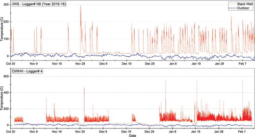
Examples of recorded IWS and OWHH stack wall temperatures and outdoor temperatures are shown in Figure 1.

Figure 1. Examples of recorded IWS and OWHH stack wall and outside temperature time series.

Based on a priori knowledge of the operation of IWSs and OWHHs, laboratory observations, and expert consultations, we developed algorithms to identify operational modes and events from the stack wall data. A general discussion of the algorithm development procedures is presented here. A more detailed discussion is available in the Supplementary Material. The purpose of this study was to assess user behavior without impacting homeowner use, therefore this study did not ask homeowners to record fueling information. Events such as loading small amounts of fuel or change in appliance settings cannot be determined from analyzing the stack temperature data set. We can assess when events occur but cannot assess which discrete actions were taken.

Outdoor wood hydronic heaters (OWHHs)

Box plots of the measured temperature of the OWHHs stack walls (Figure S-2), descriptive statistics of the measurements (Table S-1), and histograms of the normalized temperature (Figure S-3) demonstrate differing usage patterns. Depending on ambient conditions, an OWHHs can take up to several days to burn a full fuel load. In the stack wall temperature time series data, we were able to identify when a unit was loaded with new wood, but not how much wood was loaded into the appliance. Temperature patterns corresponding to specific OWHH operations were defined as follows.

At all times, the boiler is either heating the system water (in-use), or it is not (not-in-use). In-use and not-in-use modes are readily distinguishable in the temperature time series. When the boiler is in the in-use mode, the stack temperature fluctuates considerably, while in the not-in-use mode it remains flat. These usage modes are shown in Figure 2. The first pattern shows the semi-regular cycling of temperature due to the operation of the automatic air damper. A thermostat inside the building controls the call for heat by adjusting the pumps circulating hot water from the water jacket that surrounds the burner. An aquastat maintains the water temperature between set ranges. When the water temperature falls below the set range, an air damper opens, igniting the fire. The damper stays open until the temperature of the water jacket reaches the upper-temperature range. The aquastat controls lead to cyclical variations of temperatures in the boiler firebox and stack.

Figure 2. Typical OWHH stack temperature profile.

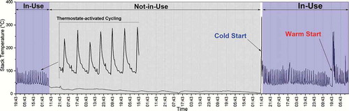
The second pattern of temperature change shown in Figure 2 occurs when the OWHH is loaded with a wood fuel charge. When fuel is added to the appliance, the stack temperature fluctuates irregularly for several minutes and then rises rapidly. The outside location of the boiler increases the cooldown speed, and the boiler cools down completely within 16–24 hours of nonuse. The loading event immediately after this period is called a “cold start.” Other loading events are called “warm starts” because they occur when the boiler is either in-use or, if not-in-use, is still warm. Both cold and warm starts are important for evaluating emissions under different start-up conditions. While operating, temperature fluctuations occur almost every hour in a cyclic pattern, due to the air damper opening and closing, as discussed above. With loading, however, temperature rise occurs only upon that event, without a specific temporal pattern.

A classification algorithm was developed to identify OWHH use patterns and events from the stack wall temperature data. First, in-use and not-in-use modes were separated based on the standard deviation of temperature. At each data point i, the standard deviation of the normalized temperature, $t_i$, is calculated, $S{D}_{t\left(i\right)}$, using a centered moving window of 60 minutes (6 time steps backward and 6 time steps forward). The window size is determined by manually inspecting the temperature time series, and it is approximately equal to the average period of one cycle of the OWHH’s thermostat function. The point $i$ is classified as not-in-use if either of the following criteria is satisfied:

C1-1: temperature at point $i$ is less than the 5^th percentile of the stack temperature distribution ($t_i<P_{0.05}\left(t\right)$)

C1-2: The standard deviation of the temperature, $S{D}_{t\left(i\right)}$, is less than the 10^th percentile of the standard deviation distribution of the entire time series ($S{D}_{t\left(i\right)}<P_{0.1}(S{D}_t$)

If none of these criteria is met, the point is classified as in-use. Based on the operation of the boiler, it is assumed that a continuous not-in-use period is greater than 10 hours. Therefore, after finishing the first round of classification, the algorithm would turn all not-in-use points that make a contiguous region less than 10 hours into in-use points. Also, to avoid noise and random temperature fluctuations when the boiler is not-in-use, all in-use periods must be at least 60 minutes long (12-time steps).

After finalizing the classification of all data points, cold and warm starts were identified by calculating the time between two consecutive in-use periods. If the periods were more than 24 hours apart, the boiler has been not in use for more than 24 hours, and the next start of combustion (i.e., beginning of the next in-use period) was marked as a cold start. If the gap was less than 24 hours, the next start was marked as a warm start.

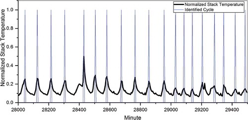
Re-loads, which occur when the boiler is in the in-use mode and the user adds wood to the active fire, are another type of warm start event. We developed an algorithm that identified re-load warm start events using a first-order differencing method. We also developed an algorithm to identify and count cycles caused by the air damper automatic activation, based on the ratio of maximum to minimum temperature in the thirty minutes around every in-use point. A detailed explanation of the algorithms is available in the Supplementary Materials for this paper. Figure 3 shows a sample of the OWHH cycle-identification algorithm output.

Figure 3. An example of the result from the OWHH cycle-identification algorithm.

Indoor wood stoves (IWSs)

As with OWHHs, IWSs are always either providing heat (in-use) or not (not-in-use). However, unlike OWHHs, IWSs are manually controlled. IWSs can be reloaded or an air adjustment can be made in response to the operator’s needs. The functional and operational differences between OWHHs and IWSs lead to more irregular temperature profiles in the IWSs, as it is shown in the box plots, histograms, and descriptive statistics provided in the Supplementary Material (Figures S-5 and S-6, and Table S-2).

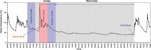
Periods of IWS in-use and not-in-use could be identified in the temperature data. In addition, we were able to separate the in-use periods into times when the fire was actively managed by the operator (referred to as the “active” mode) and times that it was not (the “inactive” mode).

During the active mode, the operator may add fuel, change appliance air settings, or manipulate/adjust the fuel. The stove temperature may cycle up and down considerably during active mode periods. When the IWS is in the inactive mode, the stack temperature is above ambient temperature and theoretically still providing heat. However, the operator is not actively engaging with the fire or appliance. An example of inactive mode is when the user loads the stove and goes to bed or work. In these instances, the IWS may continue to provide heat for a period of greater than 4–6 hours, but the temperature trend is downward.

If the inactive mode extends to more than 10 hours, it can be assumed that stove is no longer generating useful heat energy. We define this as the “not-in-use” mode. The mode that an IWS is in when the fire is re-started affects the emissions associated with the start event. If the IWS maintains some coals or internal heat from the previous operational period, re-starting the appliance may be faster and have lower emissions. Figure 4 shows use pattern and events as represented in IWS stack temperature data.

Figure 4. Typical IWS stack temperature profile with active and inactive operating modes.

Another classification algorithm was developed which utilized a first-order differencing method to identify active and inactive operational modes. We defined the inactive period as beginning when no significant fluctuations of the stack temperature (i.e., activity) had occurred for more than 4 hours. During the inactive mode, the overall temperature trend is downward, but there may be noise or random fluctuations. To avoid misclassification of the noisy data as active points, we assumed that all active periods must be at least 30 minutes long.

When the length of an inactive period exceeds 10 hours, the period is marked as a not-in-use. When the time from the last active period was greater than 10 hours but less than 24 hours, the next reloading event was considered a “warm start.” If the period exceeded 24 hours, it was assumed that the stove temperature was equal to the room temperature and, therefore, the next re-start would be a “cold start.” A detailed discussion of the derivation of this algorithm is included in the Supplementary Materials. Temperature timeseries from any stove that were used for measurement in 2015 and 2016 periods (see Table 2), were analyzed independent of each other. Because those five stoves didn’t change between the first and the second period, analyzing each period separately made it possible to compare year-to-year variations due to other factors.

Table 2. Descriptions of the indoor wood stoves (IWSs) used in the study.

Logger ID	City/Village	Nominal Output kW (kBtu/hr)	Firebox Volume liter (ft^3)	Data logging period
N1 (15)	Canton	23.4 (80)	90.6 (3.2)	1-14-15 to 3-2-15
N1 (16)				12-16-15 to 4-7-16
N2 (15)	Potsdam	18.7 (63.7)	65.1 (2.3)	1-17-15 to 2-16-15
N3 (15)	Potsdam	35.2 (120)	113.3 (4)	1-22-15 to 2-27-15
N4 (15)	Canton	N/A	N/A	1-17-15 to 2-26-15
N5 (15)	Potsdam	23.4 (80)	90.6 (3.2)	1-17-15 to 2-27-15
N5 (16)				12-15-15 to 3-22-16
N6 (15)	Hermon	14.7 (50)	N/A	1-14-15 to 2-26-15
N7 (15)	Colton	N/A	N/A	1-18-15 to 2-26-15
N8 (15)	Potsdam	14.7 (50)	56.6 (2)	1-18-15 to 2-26-15
N8 (16)				9-17-15 to 4-5-16
N9 (15)	Potsdam	16.1 (55.1)	N/A	1-17-15 to 2-26-15
N9 (16)				12-19-15 to 3-19-16
N10 (15)	Potsdam	N/A	N/A	1-17-15 to 2-27-15
N10 (16)				12-15-15 to 3-22-16
N11 (15)	Ogdensburg	N/A	N/A	1-17-15 to 2-26-15
W1 (15)	Greenacres	N/A	N/A	1-26-15 to 4-27-15
W2 (15)	Spokane	10.6 (36)	33.9 (1.2)	1-26-15 to 4-27-15
W3 (15)	Spokane	14.7 (50)	56.6 (2)	1-26-15 to 4-27-15
W4 (15)	Spokane	N/A	N/A	1-26-15 to 4-27-15
W5 (15)	Spokane	19 (65)	56.6 (2)	1-26-15 to 4-27-15
W6 (15)	Spokane	N/A	N/A	1-26-15 to 4-27-15
W7 (15)	Spokane	N/A	N/A	1-26-15 to 4-27-15
W8 (15)	Newman Lake	N/A	N/A	1-26-15 to 4-27-15
W9 (15)	Otis Orchards	N/A	N/A	1-26-15 to 4-27-15

An algorithm was developed utilizing a first-order differencing method to identify active and inactive operational modes. The algorithm identifies inactive periods and is partially reliant on the manual tuning of if-then logic, but generalized in light of its inclusion of parameters from the sample distribution for each time series. The first derivative of the temperature time series, $f^{\prime }\left(t\right)$ is approximated through $f^{\prime }\left(t\right)\approx t_{di}=\frac{t_{i+1}-t_i}{T}$, where $t_i$ is the normalized stack temperature at time step $i$, and $T$ is the 5 minute data acquisition time step. In the next step, the standard deviation, $S{D}_{td\left(i\right)}$, of the first order derivative time series, $t_d$, is calculated with one hour window size forward (12 time steps). The classification of data points starts as follows: if temperature is less than the 10^th percentile of the temperature distribution ($t_i<P_{0.1}\left(t\right)$) it is classified as inactive. Otherwise, the following criteria are checked:

C2-1: The first derivative of the temperature, $t_{di}$ is in the range of the 95^th percentile and the 1^st percentile of the $t_d$ distribution: $P_{0.01}\left(t_d\right)<t_{di}<P_{0.95}\left(t_d\right)$. This condition is to check that temperature $t_i$ is not increasing suddenly nor decreasing abruptly, which are characteristics of active mode.

C2-2: The standard deviation of the first derivative $S{D}_i$ is less than the 50^th percentile the standard deviation distribution: $S{D}_i<P_{0.5}\left(SD\right)$. This step checks that temperature fluctuations are low enough so that the point can be considered to belong to an inactive period

Initially, if both C2-1 and C2-2 are met, the point $i$ is classified as inactive, otherwise, it would be classified as active. We defined an inactive period as a period with no significant fluctuations of the stack temperate (i.e., activity) for more than 4 hours. During inactive mode, the overall temperature trend is downward, but there may be noise or random fluctuations. To avoid misclassification of the noisy data as active points, we assumed all active periods must be at least 30 minutes (6 time steps). Therefore, after finishing the initial classification, the algorithm would turn all active points that make a contiguous region less than 30 minutes into inactive points. Finally, the length of the inactive periods is used to count and classify the re-load events. When the length of an inactive period exceeds 10 hours, it is marked as a not-in-use period. If the gap between two consecutive active periods is less than 24 hours, the next start of the fire is marked as a warm start, otherwise it counts as a cold start.

Results and discussion

Outdoor wood hydronic heaters (OWHHs)

For each OWHH unit, the percentage of time in the in-use mode and the number of cold and warm starts in the fall (November-December) and winter (January-February) months are shown in Table 3. As noted in that table, the average HDD for the days that data were logged for each OWHH was considerably higher in the winter (43.9–44.8) than in the fall (26.3–28.7). OWHH1 was monitored only in the fall season. In the winter season, the three monitored units were in use continuously or almost continuously. (OWHH1 and OWHH2 were in the in-use mode 100% of the time and OWHH4 94.6% of the time during the winter monitoring period, and the users of all three of these units re-loaded their boilers every 1.5 days.

Table 3. Usage pattern of the studied OWHHs.

Logger ID	Season	Daily Average HDD	Number of Data Logging Days	% of Time In-Use	Number of Cold Starts	Number of Warm Start/Reloads	Warm Starts/Reloads per Week
OWHH1	fall	26.3	38	100	0	14	2.6
	winter	44.8	43	100	0	31	5.0
OWHH2	fall	28.7	43	97.0	2	17	2.8
	winter	44.8	33	100	0	22	4.7
OWHH3	fall	28.0	32	100	0	22	4.8
OWHH4	fall	26.4	61	50.2	4	15	1.7
	winter	43.9	42	94.6	2	28	4.7

OWHH1 and OWHH4 are the same model and make and have the same fire-box volume and output power rating (see Table 1). As discussed above, both units were in near-continuous use during the winter months. However, the in-use patterns of those two units differed in the fall, with OWHH1in use during 100% and OWHH4 only 50% of that monitoring period.

Further study of the temperature profiles of OWHH4 revealed that OWHH4 was not in operation during four multi-day periods in November and December, including three periods of approximately 10 days in length (see Figure S-4 in the Supplementary Materials). This may indicate that the residents were not at home to use the boiler during those periods. If the extended not-in-use periods are removed from the timeseries, the fuel reloading patterns become more similar. For instance, between January 2^nd and February 11^th, when both boilers were in use all the time, OWHH1 had 40 warm starts and OWHH4 had 41.

However, the cycling frequencies of those two units were very different. In the January 2^nd to February 11^th period, OWHH4 cycled an average of 22 times per day, while OWHH1 cycled 12 times a day. Since the outdoor temperature and OWHH model was the same for both locations, the cycling frequency difference may be caused by differences in transmission heat losses or in the heat demand of the building. Transmission heat loss is affected by the distance between the boiler and the building it is heating and by how well the transmission pipes are insulated. The heat demand of a building is affected by the size of the space that is being heated and by insulation of the building. We do not have sufficient information to document whether one or both of these factors is responsible for the observed difference in the cycling frequency of OWHH1 and 4. However, it is important that future testing protocols take into account the observation that widely divergent cycling frequencies can occur, even when equipment is operating under the same re-loading and ambient temperature conditions.

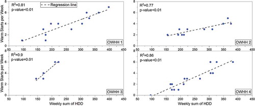
For all of the OWHHs studied, the number of warm starts per week were higher during the winter, when the outdoor temperatures were colder, than in the fall months. To further explore the effect of environmental conditions on OWHH usage patterns, the weekly heating degree days (HDD), calculated as the sum of daily HDDs, were regressed against the number of identified warm starts for each unit. Figure 5 shows a positive and statistically significant correlation between HDD and the number of warm starts for each unit with a p-value ≤ 0.01. This was expected, because, on days with a higher HDD, more energy is needed to keep the building warm.

Figure 5. Correlations between weekly heating degree days and number of identified warm starts in OWHHs.

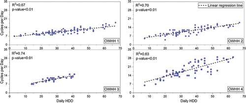
Thermostatic cycling patterns varied between OWHHs, but, for each unit, there was a significant and robust correlation between daily HDD and the number of thermostatic cycles, as shown in Figure 6. As the heat demand increases, the boiler cycles more frequently to provide energy. In OWHH1, OWHH2, and OWHH3, the average and median number of cycles per day was 11. In those three boilers the number of cycles increased by 0.13–0.24 for each unit increase in the HDD. OWHH4’s cycling pattern was considerably different. The average and median number of the cycles in OWHH4 were 18.6 and 18, respectively, and for a one unit increase in the HDD, the number of cycles increased by 0.35 units. As discussed above, the comparison of boilers OWHH1 and OWHH4 shows that a high variability in cycling patterns can occur in the same model boiler under the same weather conditions.

Figure 6. Correlations between the daily number of boilers cycles and heating degree days.

Stack wall temperatures were logged for 11 NYS IWSs and 9 WA IWS during the 2015 heating season. This afforded us the opportunity to evaluate IWS usage patterns in two regions with different climate conditions. In addition, monitoring was conducted for 5 of the NYS IWS units during the following heating season in 2016, allowing for a more in depth analysis of usage patterns over time. Details about the monthly usage patterns for each IWS, including the fraction of time in the active, inactive and not in-use modes; number of warm and cold starts; and the length of continuous active mode periods are documented in the Supplementary Materials (Tables S-3 through S-9).

Figure 7 shows the overall usage patterns (fraction of time in active, inactive and not-in-use modes) of each of the IWSs studied. Profiles for the 2015 and 2016 heating seasons are shown separately for the five stoves that were monitored in both of those periods. A wide range of usage patterns were observed. For the analysis, stoves were divided into two groups based on usage: IWSs that were in the not-in-use mode for less than 15% of the measurement period were classified as “high use” stoves and the remaining units as “low use” devices. Using that criterion, five stoves (seven stove-years) were classified as high use IWSs, as shown in Figure 6. Only one of the high use IWS was located in WA; however, that stove, W1, exhibited the highest fraction of active use of all of the stoves.

Figure 7. The overall fraction of usage modes for IWSs.

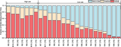
Figure S-7 compares the year-to-year usage patterns for the five NYS IWS units which were monitored during both the 2015 and 2016 heating seasons. The stoves ranked in the same order of high to low usage in both periods. However, the in-use fraction of all of the stoves was lower in the 2016 heating season than in the 2015 heating season. As discussed below, this difference can be linked, at least in part, to the milder temperatures (lower HDD) observed in the second heating season, although other factors, including fuel oil prices, may also have played a role in the decreased operation of the IWS units in the second heating season. Note that data were logged for a longer period in the 2016 than in the 2015 heating season. A more detailed analysis of these data is presented below.

All NYS and WA IWSs were monitored throughout the month of February 2015. NYS was considerably colder that month (total monthly HDD of 1653) than WA (861 HDD). Figure 8 shows the fraction of time that the NYS and WA stoves were in the active and not-in-use modes that month. The NYS stoves spent considerably less time in the not-in-use mode than the WA stoves, as would be expected, given the ambient temperature difference. The median fraction of not-in-use time for the NYS IWS in February 2015 was 14%, as compared to 56% for the WA stoves. Conversely, the median fraction of time in the active mode was considerably higher for the NYS stoves (60%) than for the WA stoves (34%). Note, however, that a wide range of usage patterns were observed among the stoves in each region; the in-use percentage for the NYS IWS ranged from 31-96% that month, while the WA units were in-use between 6 and 92% of that period.

Figure 8. Comparison of usage patterns of NYS and WA stoves in February 2015.

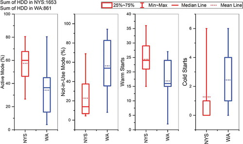
Figure 8 also shows the distribution of the number of cold and warm starts during February 2015 for the IWSs in NYS and WA. On average, the NYS IWSs had more warm starts and fewer cold starts than the WA stoves, which is expected, since the NYS stoves were more often in-use. However, a wide range of frequencies of both warm starts and cold starts was observed in both states. Three of the high-use IWSs in NYS and the one WA high-use IWS experienced no cold starts that month. IWS N4, a low-use NYS stove, recorded the highest number of cold starts, an average of 1.65 per week, that month. IWSs in NYS recorded a range of 16–36 (mean 26) warm starts that month, while that range was 1.6– 22 (mean 14) for the WA IWSs.

Note that the methodology used in our study cannot identify fuel reloads that occur when the fire in the stove is still actively burning. Therefore, the number of warm and cold starts that we documented underestimated the actual number of refueling events for IWSs that are refueled while the flame is still active. A study by Wöhler et al. (2016) suggests that this underestimation may be significant. In that study, 45% of the wood stove users surveyed said that they refilled their stoves when fuel was still strongly burning or small flames were visible.

The distributions of the number of warm start events per day for high and low use ISWs are shown in Figure 9. As expected, more warm starts were observed in the high-use than in the low-use stoves. High-use stoves had a median of 1.0 warm start event per day, as compared to 0.7 for the low-use IWS. Since, as discussed above, the number of warm starts does not capture refueling events that occur during periods of active management, this finding is consistent with the findings of the Wöhler et al. (2016) survey-based study, which determined that the majority of firewood stove users in Europe refilled their stoves 2–5 times a day during high use seasons and 0–1 times per day during low use periods.

Figure 9. Ranges of warm start event frequency and continuous active mode duration for IWSs.

As discussed in the Methodology section, the classification of the fuel loading events captured by our methodology as “warm starts” or “cold starts” was based on the duration of time between two consecutive active periods. Warm starts generally occur when the stove is the inactive mode, and cold starts when the stove is inactive or not-in-use. As shown in Figure 10, we saw a relatively strong and significant linear correlation, with a p-value < .01, between the portion of time that a stove was in the inactive mode and the frequency of warm starts for both high and low-use IWS.

Figure 10. Relationship between the share of inactive mode and warm and cold starts.

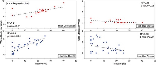
The number of cold start events observed was inversely correlated with the portion of the time that a stove was in the inactive mode but, as shown in Figure 10, that relationship was weaker than with warm starts (p-value < .1). The number of cold start events did not significantly correlate with the portion of time in the not-in-use mode. Note that a cold start would occur only once after a period of not in-use, but the length of nonuse periods varied widely.

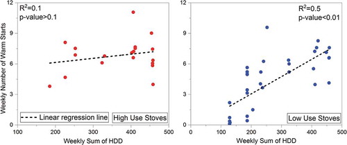
A regression analysis was performed to determine the relationship between ambient temperature, as represented by HDD, and the number of observed warm and cold start events. As shown in Figure 11, we saw a significant (p < .01) positive correlation between HDD and warm start events for low-use, but not for high-use IWSs. It is possible that we would have seen a correlation between those variables in high-use IWSs also if we were able to capture refueling events that occurred when the stoves were in active use. There was no significant relationship between the weekly HDD and the number of cold starts in either of the use categories. Correlation analyses were repeated with other weather parameters, such as daily average and minimum outside temperatures. None of the usage parameters correlated with usage parameters

Figure 11. Relationship between the weekly sum of heating degree days and frequency of warm start events.

Indoor wood stoves (IWSs)

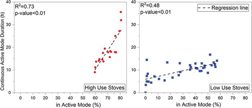
Figure 9 also shows the distribution of the average durations of continuous active mode periods for high and low use ISWs. The length of the active modes for the high-use stoves (median 17 hours) was considerably higher than for the low-use units (12 hours). Note, however, that wide ranges in active mode lengths were recorded for stoves in both the low-use (1.5– 51 hours) and high-use (1.5– 134 hours) categories. While it makes intuitive sense that the length of continuous time that an IWS was maintained in the active mode may be influenced by the outside temperature, there was no clear relationship between HDD and this variable. The longest continuous period of active operation, 134 hours (5.6 days) was recorded by the high-use WA stove in February 2015. As shown in Figure 12, the duration of a stove’s active mode periods correlated well with the percentage of time that the stove was in the active mode for both high-use and low-use stoves.

Figure 12. Correlation between the share of active mode and the mean duration of continuous active periods.

Intertemporal spacing of active periods is an indicator patterns of management of the IWS units. An analysis of this variable determined that the probability that a stove was not active for a relative short period (less than 5–6 hours) was similarly high for almost all devices, regardless of their long-term usage patterns. However, the likelihood of observing longer gaps between two consecutive active periods is noticeably different for high and low use units. There is only a 2% probability that a high-use stoves would not be active for a period of 24 hours, while that probability for low use stoves is 12%. A more detailed explanation of this analysis is available in the Supplementary Materials (Figure S-8).

The monitoring of five of the NYS IWS for a total of six months over two heating seasons provided us with an additional opportunity to explore IWS usage patterns and factors that may affect those patterns. Table 4 shows year-to-year comparison of the usage patterns of five stoves. The relationship between usage of those five IWSs and temperature was evaluated by regressing the percentage of time that each stove was in-use for each of the six months that data were logged against monthly HDD. As shown in Figure S-9, stoves N5 and N10 were in high-use in all months, an indication that those stoves are used as a significant source of heat in those residences. N1 and N8, which showed a more variable usage pattern that correlated more strongly with HDD, were likely used as a supplemental heat source, particularly in colder periods.

Table 4. Average usage patterns of the stoves in NYS with two years of measurement.

	Active		Inactive		Not in Use		Warm Starts per Week		Cold Starts per Week
Heating Season	2014-15	2015-16	2014-15	2015-16	2014-15	2015-16	2014-15	2015-16	2014-15	2015-16
N5	0.78	0.74	0.20	0.21	0.02	0.05	5.54	6.19	0.12	0.18
N10	0.74	0.70	0.22	0.23	0.03	0.07	6.78	7.15	0.13	0.00
N9	0.69	0.55	0.24	0.23	0.07	0.23	6.86	7.60	0.14	0.38
N1	0.54	0.39	0.22	0.12	0.24	0.49	7.36	5.06	0.12	0.71
N8	0.44	0.30	0.13	0.04	0.43	0.66	6.05	4.16	0.78	1.07

As discussed above and shown in Figures 7 and 8, although the ranking of the five stoves by in-use percentage was the same for both heating seasons, all stoves were in-use for a lower percentage of time in the 2016 heating season than in the 2015 season. The higher HDD associated with the colder temperatures in the 2015 heating season monitoring period can partially explain this difference. However, additional factors must also be considered.

In St. Lawrence County, where stoves 1, 8, 9, and 10 were located, utility gas and fuel oil are the most common house heating fuels (NYSERDA 2019). The average price of utility gas in NYS was about 3% higher in the 2016 study period than in the 2015 period, rising from an average of 10.1 $/MCF in the 2015 heating season to 10.4 $/MCF in the 2016 period. However, the average price of No. 2 residential heating oil moved strongly in the opposite direction, decreasing from an average of $3.21/gallon during the 2014–15 heating season to $2.46/gallon in the 2015–16 heating season (EIA 2019a). Although data obtained from homeowner in the study did not include primary fuel use, there is limited access to natural gas in the study area, so home heating oil is the typical fuel. Although the effect cannot be quantified, it is likely that the considerably lower price of oil in the second heating season may have contributed to reduced woodburning in that season.

Note that, although use of all five of those NYS IWSs seem to have been affected by some combination of lower HDD and lower fuel oil prices in the 2016 heating season, the usage patterns of those units are very different from each other. This suggests that usage of each IWS was affected by both external factors (e.g., heat demand and fuel prices) and by factors that are individual to the household that it heats. The same model of stove may be subject to a wide variety of usage patterns, depending on the region in which it is deployed, ambient temperatures and fuel prices during a heating season, whether it is being used as a significant source of household heat, and the behavior of the owner. Emissions testing protocols should, to the extent possible, represent the range of operating conditions that the stove may encounter.

To further investigate the variability of IWS usage patterns, a weekday/weekend analysis was performed. Table 5 shows the weekday-weekend patterns in NYS and WA. In the NYS stoves, the share of the in-use mode increased over the weekends, while it decreased in the WA stoves. For the NYS stoves, appliances in the “high use” category showed a considerably larger increase in time in the in-use mode during the weekend than the “low use” devices. This behavior is consistent with the assumption that the users of the high use stoves rely more on their stoves for home heating, and therefore, would use them more when they are home on weekends. The results of weekday-weekend analysis of the NYS stoves in this research are consistent with a previous study by Wang et al. (2011) which measured ambient residential wood combustion particles in Rochester, NY. The winter diurnal pattern of PM2.5 in that study showed an evening peak that was particularly enhanced on weekends. However, this does not explain why stove users in WA decreased their usage during weekends.

Table 5. Weekday/weekend analysis of IWS in-use modes.

		% of the In-Use mode
State	Use Category	Weekday	Weekend	Change
NY	High	71.6%	78.6%	9.4%
	Low	45.9%	47.0%	2.4%
WA	High	85.6%	84.6%	−1.1%
	Low	12.7%	10.6%	−17.9%

Based on the in-home usage patterns of the IWS and OWHHs in this study, it is clear that the current certification testing methodology, which uses steady-state conditions, does not reflect in-use practices. In the home, thermostatically controlled appliances display cyclic on/off operations in response to heating calls. OWHHs fire in a full-output mode for an extended period, but once the thermostat is satisfied, the burner will shut off. We documented that, when heat demand is higher, the frequency of the OWHH boiler automatic cycling and the number of warm starts is higher. Therefore, the current certification testing methodology, which does not require appliance cycling to simulate varying heat demands, is not reflective of real-life use. In addition, OWHH loading patterns vary according to homeowner preference, and those patterns are also not reflected in the current testing methodology, which is based on the burn of a full fuel load.

HDD is correlated with overall use of IWS units and, for lower-use stoves, with the number of warm starts that the stove experiences. The warmer temperatures (lower HDD) in WA largely explains fact that all but one of the units monitored in that state were in the low-use category. HDD differences, along with a drop in the price of fuel oil, likely contributed to the reduced use of NYS stoves in the 2016 heating season, as compared to 2015.

However, those factors do not explain the wide variation between the usage patterns of the stoves studied. In February 2015, when all WA and NY stoves were monitored, the one high-use WA stove had a higher percentage of time in active use and the longest period of continue active of any of the stoves, despite the fact that the HDD was more approximately 2.5 times higher in NYS than in WA during that period. The five NYS stoves that were monitored over two heating seasons all showed some decrease use in the second, warmer year; however, those stoves reflected a wide range of use patterns. It is essential that testing procedures be developed that represent the full range of operation.

The impact of start-up events is critical parameter in characterizing in-field performance. Laboratory studies have identified two key periods as driving emissions performance, start-ups and large loads and low air settings (typical use pattern for overnight burns) (EPA 2012). Warm starts occurred in the stoves in our study up to eleven times per week and cold starts up to seven times per month. Neither these start-up events nor the large load/low air settings typical of overnight use are included in current IWS certification test protocols.

The methodology of this research is a novel approach to understand and quantify usage patterns without influencing user behavior. The results from this study, along with the conduct of similar studies in other regions, usage surveys, and emission testing evaluations, can be used to design certification testing methodology that is representative of the range of likely operating conditions in the field. This work is essential, given the disproportionate impact of residential wood burning on air quality.

Conclusion

Compared to OWHHs, the usage pattern variability of the IWSs is higher and the dependency on environmental conditions is weaker. In summary, the current certification testing practice of burning a single fuel configuration at one heat setting for the entire fuel load, with no start-up or reloading events, does not reflect the usage patterns identified in this study. The observed in-home usage patterns are highly variable, and this variability persists regardless of the device’s location or type. In recognition of this observation, current steady-state testing should be replaced with a test method that incorporates a variety of burn conditions and fuel load configurations that mimics the variable operating patterns. This would reflect more realistic real-life performance values during certification testing. This would be a departure from current certification practice, but would better reflect device performance in actual home use.

Acknowledgment

The authors thank Rod Tinnemore, Washington Department of Ecology, Dr. Thomas Butcher and Dr. Rebecca Trojanowski of Brookhaven National Lab for helpful comments and review of the analysis approach, and Dr. Phil Hopke and Mauro Masiol of Clarkson University for helping deploy the temperature data loggers and data collection. Any opinions expressed in this article do not necessarily reflect those of NYSERDA or the State of New York, and reference to any specific product, service, process, or method does not constitute an implied or expressed recommendation or endorsement of it.

Disclosure statement

No potential conflict of interest was reported by the authors.

Supplementary material

Supplementary material for this article can be accessed on the publisher’s website.

Additional information

Funding

This work was supported by the New York State Energy Research and Development Authority (NYSERDA) under Agreement Nos. [34263B and 63035].

Notes on contributors

Mahdi Ahmadi

Mahdi Ahmadi is an Environmental and Energy Analyst at Northeast States for Coordinated Air Use Management (NESCAUM) in Boston, MA.

Josh Minot

Josh Minot is in the Ph.D. program at the University of Vermont Complex Systems Center

George Allen

George Allen is the Chief Scientist at Northeast States for Coordinated Air Use Management (NESCAUM) in Boston, MA.

Lisa Rector

Lisa Rector is a Policy and Program Director at Northeast States for Coordinated Air Use Management (NESCAUM) in Boston, MA.

References

- Bari, M. A., G. Baumbach, B. Kuch, and G. Scheffknecht. 2009. Wood smoke as a source of particle-phase organic compounds in residential areas. Atmos. Environ. 43 (31):4722–32. doi:10.1016/j.atmosenv.2008.09.006.
- Boman, C., B. Forsberg, and T. Sandström. 2006. Shedding new light on wood smoke: A risk factor for respiratory health. Eur. Respiratory Soc. 27:446–47. doi:10.1183/09031936.06.00000806.
- Brandelet, B., C. Rose, C. Rogaume, and Y. Rogaume. 2018. Impact of ignition technique on total emissions of a firewood stove. Biomass Bioenergy 108:15–24. doi:10.1016/j.biombioe.2017.10.047.
- Central Boiler. 2018. Classic edge products homepage. Accessed May 9, 2019. https://centralboiler.com/products/classic-edge.
- Denier Van Der Gon, H. A. C., R. Bergström, C. Fountoukis, C. Johansson, S. N. Pandis, D. Simpson, and A. J. H. Visschedijk. 2015. Particulate emissions from residential wood combustion in Europe–revised estimates and an evaluation. Atmos. Chem. Phys. 15 (11):6503–19. doi:10.5194/acp-15-6503-2015.
- EIA, (U.S. Energy Information Administration). 2018. Residential energy consumption survey. Accessed September 25, 2017. https://www.eia.gov/consumption/residential/data/2015/hc/php/hc6.7.php.
- EIA, (U.S. Energy Information Administration). 2019a. Weekly New York no. 2 heating oil residential price. Accessed May 9, 2019. https://www.eia.gov/dnav/pet/hist/LeafHandler.ashx?n=PET&s=W_EPD2F_PRS_SNY_DPG&f=W.
- EIA, (U.S. Energy Information Administration). 2019b. Wood and wood waste. Accessed May 1, 2019. https://www.eia.gov/energyexplained/index.php?page=biomass_wood.
- Englert, N. 2004. Fine particles and human health—a review of epidemiological studies. Toxicol. Lett. 149 (1–3):235–42. doi:10.1016/j.toxlet.2003.12.035.
- EPA, (U.S. Environmental Protection Agency). 2012. Environmental, energy market, and health characterization of wood-fired hydronic heater technologies. Albany: New York State Energy Research and Development Authority. https://www.nyserda.ny.gov/-/media/Files/Publications/Research/Environmental/Wood-Fired-Hydronic-Heater-Tech.pdf.
- EPA, (U.S. Environmental Protection Agency). 2014. National Emission Inventory (NEI) data. https://www.epa.gov/air-emissions-inventories/2014-national-emissions-inventory-nei-data.
- EPA, (U.S. Environmental Protection Agency). 2015a. Regulatory Impact Analysis (RIA) for residential wood heaters NSPS revision. https://www.epa.gov/sites/production/files/2015-02/documents/20150204-residential-wood-heaters-ria.pdf.
- EPA, (U.S. Environmental Protection Agency). 2015b. Standards of performance for new residential wood heaters, new residential hydronic heaters and forced-air furnaces. Final Rule, 80 Fed. Regist. 50.
- Fachinger, F., F. Drewnick, R. Gieré, and S. Borrmann. 2017. How the user can influence particulate emissions from residential wood and pellet stoves: Emission factors for different fuels and burning conditions. Atmos. Environ. 158:216–26. doi:10.1016/j.atmosenv.2017.03.027.
- Glasius, M., M. Ketzel, P. Wåhlin, B. Jensen, J. Mønster, R. Berkowicz, and F. Palmgren. 2006. Impact of wood combustion on particle levels in a residential area in Denmark. Atmos. Environ. 40 (37):7115–24. doi:10.1016/j.atmosenv.2006.06.047.
- Herich, H., M. F. D. Gianini, C. Piot, G. Močnik, J.-L. Jaffrezo, J.-L. Besombes, A. S. H. Prévôt, and C. Hueglin. 2014. Overview of the impact of wood burning emissions on carbonaceous aerosols and PM in large parts of the Alpine region. Atmos. Environ. 89:64–75. doi:10.1016/j.atmosenv.2014.02.008.
- Houck, J. E., and P. E. Tiegs. 1998. Residential wood combustion technology review. Volume 1. Technical report, U.S. Environmental Protection Agency, Washington, DC. https://cfpub.epa.gov/si/si_public_record_Report.cfm?Lab=NRMRL&dirEntryID=90399.
- Johansson, L. S., B. Leckner, L. Gustavsson, D. Cooper, C. Tullin, and A. Potter. 2004. Emission characteristics of modern and old-type residential boilers fired with wood logs and wood pellets. Atmos. Environ. 38 (25):4183–95. doi:10.1016/j.atmosenv.2004.04.020.
- Maenhaut, W., R. Vermeylen, M. Claeys, J. Vercauteren, C. Matheeussen, and E. Roekens. 2012. Assessment of the contribution from wood burning to the PM10 aerosol in Flanders, Belgium. Sci. Total Environ. 437:226–36. doi:10.1016/j.scitotenv.2012.08.015.
- McDonald, J. D., B. Zielinska, E. M. Fujita, J. C. Sagebiel, J. C. Chow, and J. G. Watson. 2000. Fine particle and gaseous emission rates from residential wood combustion. Environ. Sci. Technol. 34 (11):2080–91. doi:10.1021/es9909632.
- Morris, R. D. 2001. Airborne particulates and hospital admissions for cardiovascular disease: A quantitative review of the evidence. Environ. Health Perspect. 109 (suppl 4):495–500. doi:10.1289/ehp.01109s4495.
- Naeher, L. P., M. Brauer, M. Lipsett, J. T. Zelikoff, C. D. Simpson, J. Q. Koenig, and K. R. Smith. 2007. Woodsmoke health effects: A review. Inhal. Toxicol. 19 (1):67–106. doi:10.1080/08958370600985875.
- NYSERDA, (New York State Energy Research and Development Authority). 2019. Monthly average price of natural gas – Residential. Accessed September 25, 2019. https://www.nyserda.ny.gov/Researchers-and-Policymakers/Energy-Prices/Natural-Gas/Monthly-Average-Price-of-Natural-Gas-Residential.
- Oehler, H., R. Mack, H. Hartmann, S. Pelz, M. Wöhler, C. Schmidl, and G. Reichert. 2016. Development of a test procedure to reflect the real life operation of pellet stoves. ETA-Florence Renewable Energies. Paper published in 24th European Biomass Conference and Exhibition, Amsterdam, 738–47.
- Pettersson, E., C. Boman, R. Westerholm, D. Boström, and A. Nordin. 2011. Stove performance and emission characteristics in residential wood log and pellet combustion, part 2: Wood stove. Energy Fuels 25 (1):315–23. doi:10.1021/ef1007787.
- Piazzalunga, A., C. Belis, V. Bernardoni, O. Cazzuli, P. Fermo, G. Valli, and R. Vecchi. 2011. Estimates of wood burning contribution to PM by the macro-tracer method using tailored emission factors. Atmos. Environ. 45 (37):6642–49. doi:10.1016/j.atmosenv.2011.09.008.
- Pope, C. A., III, and D. W. Dockery. 2006. Health effects of fine particulate air pollution: Lines that connect. J. Air Waste Manage. Assoc. 56 (6):709–42. doi:10.1080/10473289.2006.10464485.
- Reichert, G., and C. Schmidl. 2018. Advanced test methods for firewood stoves: Report on consequences of real-life operation on stove performance. IEA Bioenergy (Wieselburg). http://task32.ieabioenergy.com/wp-content/uploads/2018/10/IEA-Bioenergy-Task-32-Test-Methods.pdf.
- Reichert, G., C. Schmidl, W. Haslinger, M. Schwabl, W. Moser, S. Aigenbauer, M. Wöhler, and C. Hochenauer. 2016. Investigation of user behavior and assessment of typical operation mode for different types of firewood room heating appliances in Austria. Renewable Energy 93:245–54. doi:10.1016/j.renene.2016.01.092.
- Reichert, G., H. Hartmann, W. Haslinger, H. Oehler, R. Mack, C. Schmidl, C. Schön, M. Schwabl, H. Stressler, and R. Sturmlechner. 2017. Effect of draught conditions and ignition technique on combustion performance of firewood roomheaters. Renewable Energy 105:547–60. doi:10.1016/j.renene.2016.12.017.
- Schieder, W., A. Storch, D. Fischer, P. Thielen, A. Zechmeister, S. Poupa, and S. Wampl. 2013. Luftschadstoffausstoß von Festbrennstoff-Einzelöfen–Untersuchung des Einflusses von Festbrennstoff-Einzelöfen auf den Ausstoß von Luftschadstoffen. Wien: Umweltbundesamt GmbH.
- Schmidl, C., M. Luisser, E. Padouvas, L. Lasselsberger, M. Rzaca, C. R.-S. Cruz, M. Handler, G. Peng, H. Bauer, and H. Puxbaum. 2011. Particulate and gaseous emissions from manually and automatically fired small scale combustion systems. Atmos. Environ. 45 (39):7443–54. doi:10.1016/j.atmosenv.2011.05.006.
- Shen, G., M. Xue, S. Wei, Y. Chen, Q. Zhao, B. Li, H. Wu, and S. Tao. 2013. Influence of fuel moisture, charge size, feeding rate and air ventilation conditions on the emissions of PM, OC, EC, parent PAHs, and their derivatives from residential wood combustion. J. Environ. Sci. 25 (9):1808–16. doi:10.1016/S1001-0742(12)60258-7.
- U.S. Census Bureau. 2019. 2017 data from American Community Survey 5-Year Estimates, House Heating Fuel, ID B25040. U.S. Census Bureau. Accessed April 30, 2019.
- Vicente, E. D., M. A. Duarte, A. I. Calvo, T. F. Nunes, L. Tarelho, and C. A. Alves. 2015a. Emission of carbon monoxide, total hydrocarbons and particulate matter during wood combustion in a stove operating under distinct conditions. Fuel Process. Tech. 131:182–92. doi:10.1016/j.fuproc.2014.11.021.
- Vicente, E. D., M. A. Duarte, A. I. Calvo, T. F. Nunes, L. A. C. Tarelho, D. Custódio, C. Colombi, V. Gianelle, A. Sanchez de la Campa, and C. A. Alves. 2015b. Influence of operating conditions on chemical composition of particulate matter emissions from residential combustion. Atmos. Res. 166:92–100. doi:10.1016/j.atmosres.2015.06.016.
- Wang, Y., P. K. Hopke, O. V. Rattigan, X. Xia, D. C. Chalupa, and M. J. Utell. 2011. Characterization of residential wood combustion particles using the two-wavelength aethalometer. Environmental Science & Technology 45 (17):7387–7393.
- Wöhler, M., J. S. Andersen, G. Becker, H. Persson, G. Reichert, C. Schön, C. Schmidl, D. Jaeger, and S. K. Pelz. 2016. Investigation of real life operation of biomass room heating appliances–Results of a European survey. Appl. Energy 169:240–49. doi:10.1016/j.apenergy.2016.01.119.
- Wöhler, M., and S. K. Pelz. 2017. The “beReal” project the firewood method - 19th of January 2017 in the frame of the 5th central European biomass conference, Graz, Austria. Accessed December 4, 2019. http://www.bereal-project.eu/uploads/1/3/4/9/13495461/13.40_the_firewood_method.pdf.