Wildfire and prescribed burning impacts on air quality in the United States

ABSTRACT

Air quality impacts from wildfires have been dramatic in recent years, with millions of people exposed to elevated and sometimes hazardous fine particulate matter (PM_2.5) concentrations for extended periods. Fires emit particulate matter (PM) and gaseous compounds that can negatively impact human health and reduce visibility. While the overall trend in U.S. air quality has been improving for decades, largely due to implementation of the Clean Air Act, seasonal wildfires threaten to undo this in some regions of the United States. Our understanding of the health effects of smoke is growing with regard to respiratory and cardiovascular consequences and mortality. The costs of these health outcomes can exceed the billions already spent on wildfire suppression. In this critical review, we examine each of the processes that influence wildland fires and the effects of fires, including the natural role of wildland fire, forest management, ignitions, emissions, transport, chemistry, and human health impacts. We highlight key data gaps and examine the complexity and scope and scale of fire occurrence, estimated emissions, and resulting effects on regional air quality across the United States. The goal is to clarify which areas are well understood and which need more study. We conclude with a set of recommendations for future research.

Implications

In the recent decade the area of wildfires in the United States has increased dramatically and the resulting smoke has exposed millions of people to unhealthy air quality. In this critical review we examine the key factors and impacts from fires including natural role of wildland fire, forest management, ignitions, emissions, transport, chemistry and human health.

Introduction

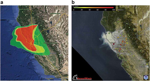
Large wildfires in the United States are becoming increasingly common, and smoke from these fires is a national concern. Figure 1 shows impacts from large wildfires that burned in the western U.S. in summer of 2017. These fires generated smoke plumes that were transported across North America, resulting in measured PM_2.5 (particulate matter with aerodynamic diameter ≤2.5 micrometers) concentrations that reached Unhealthy to Hazardous levels in many areas, based on National Ambient Air Quality Standard definitions.

Daniel A. Jaffe

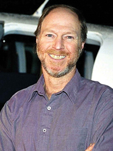
Figure 1. (A) (top) Observed smoke on September 4, 2017. (Top) NASA Worldview (https://worldview.earthdata.nasa.gov/) image showing fire hotspot detections from the VIIRS and MODIS satellite instruments, along with visible satellite imagery from the VIIRS instrument between 1200–1400 local time. Bright white areas are clouds; grayer areas are smoke. (B) (Bottom) 24-hour average PM_2.5, shown as the corresponding Air Quality Index (AQI) level category colors, based on surface PM sensors collected in the EPA’s AirNow system (https://www.airnow.gov/).

Fires emit PM directly along with hundreds of gaseous compounds. The gaseous compounds include nitrogen oxides (NOx), carbon monoxide (CO), methane (CH₄), and hundreds of volatile organic compounds (VOCs), including a large number of oxygenated VOCs (OVOCs). This chemical complexity makes wildfire smoke very different from typical industrial pollution. A key challenge for understanding fire impacts on air quality is the large variability from fire to fire in both the quantity and composition of emissions. Emissions can vary as a function of the amount and type of fuel (Prichard et al. 2019a), meteorology, and burning conditions. These variations give rise to large uncertainties in the emissions from individual fires (Larkin et al. 2012). Once emitted, wildfire smoke undergoes chemical transformations in the atmosphere, which alters the mix of compounds and generates secondary pollutants, such as ozone (O₃) and secondary organic aerosol (SOA).

Wildland fire is an essential ecological process integral to shaping most North American ecosystems. Wildland ecosystems, broadly, include both forests and rangelands, which are distributed across the spectrum of rural to urban environments; forests cover 360 million hectares (ha) and rangelands cover 308 million ha, 33% and 29% of land in the United States, respectively. The scope and scale of fire within these environments vary widely, with consequences for both emissions and effects of smoke.

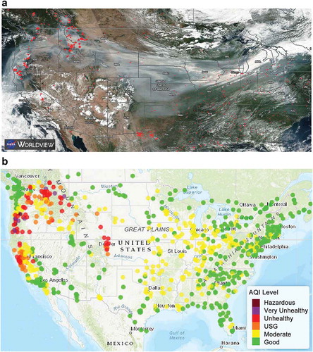
Figure 2 shows the progression of fire in the U.S. throughout the year 2017 as seen by satellite detections. In winter, fires are found mainly in the Southeast, typically as prescribed low-intensity understory burns to maintain longleaf pine and other forest savanna systems. As spring approaches, fire detections move north, with increased prescribed fire activity across the central U.S. in many rangelands. In summer, wildfire season peaks, especially in the western U.S. Late fall can also be a time of many fires in California and the Southeast. This progression of fire throughout the seasons and ecosystems across the U.S. has implications for the overall quantity and specific chemistry of the emitted smoke.

Figure 2. Progression of fires throughout the year using 2017 MODIS hotspot fire detections.

Humans have a profound influence on both the use and suppression of wildland fire. It is difficult to separate human influence from the natural occurrence of fire on the landscape (Pyne 1997). For example, Native Americans used fire as a tool for agriculture and to manage wildlife habitat and hunting grounds. These frequent, low-intensity fires may have substantially affected the landscape across the U.S, but modern management practices, especially fire suppression efforts, probably have been more important in changing the forest structure (Ryan, Knapp, and Varner 2013). The result through the 1900 s has been less fire on the landscape than in pre-settlement times (Leenhouts 1998), and therefore, likely less smoke in the air (Brown and Bradshaw 1994). Recent episodes of smoke across extensive landscapes, driven by large wildfires, may therefore to some extent be a return to pre-suppression levels.

A number of studies have documented the importance of climate change on the increasing frequency and size of fires in the western U.S. Large fires are increasing in the West (Dennison et al. 2014). Rising temperatures affect fuel aridity and the length of the fire season (Abatzoglou and Williams 2016), the amount of snow, the timing of snowmelt (Westerling 2016), and relative humidity, which has been related to the increasing trend of area burned in California (Williams et al. 2019). However, the relationship between climate and human influences is complex and not all fires should be attributed to climate change. For example, Mass and Ovens (2019) suggested that the 2017 Wine Country fires in northern California likely had little influence from recent climate change. Littell et al. (2009) found that the effect of climate change on area burned can vary with the ecosystem and fuels.

Complicating the role of climate change are the effects of invasive species (Fusco et al. 2019) and direct human ignitions. These ignitions are estimated to be responsible for over 80% of wildfires, by number, across the U.S., excluding prescribed and management fires (Balch et al. 2017). Human ignition sources include vehicles, construction equipment, power lines, fireworks, camping, arson, and others. However, in the Intermountain West, lightning appears to be the dominant cause for ignitions (Balch et al. 2017). Human ignitions have expanded the length of the wildfire season, but climate and human presence are interrelated factors (Syphard et al. 2017).

Crop-residue burning is common across the U.S. to remove or reduce biomass. Prescribed burning – planned ignition in accordance with applicable laws, policies, and regulations to meet specific objectives (NWCG 2018) – also occurs for multiple reasons, including to reduce fuel loading and ecosystem health. Both crop-residue fires and prescribed burning tend to occur in the non-summer months, and, depending upon the state, they may be permitted under a smoke management program to ensure that smoke exposure will not exceed air quality standards or affect sensitive populations.

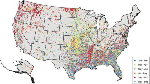
Although 98% of wildfires are suppressed before reaching 120 ha (Calkin et al. 2005), the annual area burned by wildfires is increasing. Figure 3 shows the large interannual variability in wildfire area burned and the substantial increase in area burned and federal suppression costs between 1999 and 2018. In those two decades, wildland fires burned an average of 2.8 million ha per year, which is more than double the annual amount that burned in the two decades before 1998 (National Interagency Fire Center [NIFC], 2019). This comparison indicates that a small number of fires are expanding in size and greatly increasing the area burned.

Figure 3. Total U.S. wildfire area burned (ha) and federal suppression costs for 1985–2018 scaled to constant (2016) U.S. dollars. Trends for both wildfire area burned and suppression indicate about a four-fold increase over a 30-year period.

Although the area burned globally appears to be declining (Andela et al. 2017), in the U.S. the area burned by wildfires is on the rise, and federal costs of wildfire suppression have risen substantially along with area burned. In 2018, federal suppression costs were the highest ever, at over 3 USD billion (NIFC, 2019). As towns and cities have grown and spread deeper into the wildlands, creating a larger wildland-urban interface (WUI), an increasing share of resources for forest management and firefighting effort has gone toward protecting human developments.

In recent years, smoke from large fires has caused extreme concentrations of PM_2.5 and O₃, especially in the western U.S. (Gong et al. 2017; Laing and Jaffe 2019; Mass and Ovens 2019). The highest PM_2.5 concentrations ever observed in many western cities were seen in the summers of 2017 or 2018, due to wildfires, with some daily PM_2.5 values of over 500 µg/m³ (see box: The relationship between fire activity and smoke, 2004–2018). The U.S. has made steady progress in reducing air pollution from industrial and vehicle emissions, but the recent increase in wildland fires has slowed or even reversed this progress in some parts of the country (McClure and Jaffe 2018).

Although much of the recent attention on wildfires has focused on the western U.S., large fires also burn in the southeastern U.S. In November 2016, large wildland fires burned in Tennessee, North Carolina, South Carolina, and Georgia, generating PM_2.5 concentrations exceeding 100 µg/m³ in many cities. The smoke and elevated PM_2.5 persisted across the region for weeks. Prescribed and crop-residue burning are also common in the Southeast, in some cases with consequences to health (Huang et al. 2019).

As smoke plumes move over populated areas, they can elevate PM_2.5 and/or O₃ levels over health standards. Large and extended wildfires can be associated with respiratory issues and premature mortality (e.g., Liu et al. 2015a; Reid et al. 2019). The plumes can affect regions directly and/or mix with other urban pollutants. In the U.S., the Clean Air Act of 1963 was enacted to protect public health and welfare. In 1970 the U.S. Environmental Protection Agency (EPA) established the National Ambient Air Quality Standards (NAAQS) for six criteria pollutants. The criteria pollutants most relevant to wildland fire emissions are PM_2.5, O₃, and CO. For daily average PM_2.5, the current primary standard is 35 µg/m³ at the 98^th percentile, averaged over three years. For O₃, the current primary standard is 0.070 ppm for the annual fourth-highest daily maximum 8-hour concentration (MDA8), averaged over three years. For CO, the current primary standards are 9 ppm for an 8-hour averaging time, and 35 ppm for a one-hour averaging time, not to be exceeded more than once per year. Although CO from fires is rarely a concern to the public, it can affect wildland firefighters, and recent work analyzes exposure in terms of National Institute of Occupational Safety and Health (NIOSH) standards (Henn et al. 2019). Smoke plumes from wildland fires have caused substantial exceedances of the EPA standards for both PM_2.5 and O₃, but a state may try to exclude these data from regulatory consideration under the exceptional events rule (See Section 8, Regulatory context for air quality management, for further discussion).

The EPA’s National Emission Inventory (NEI) is generated every three years and includes all significant categories of emissions for the major pollutants. The 2011 and 2014 NEI show that wildland fire emissions represented approximately 32% of the total primary PM_2.5 emissions in the U.S. (Larkin et al. 2020). Liu et al. (2017a) estimated that, in 2011–2015, fires in 11 western states emitted on average twice as much primary PM_2.5, compared to the annual emissions from all industrial sources in the region. Although prescribed burning remains relatively constant interannually (5.03 million ha in 2011, 4.42 million ha in 2014), wildfires are subject to large interannual variability (4.32 million ha in 2011, 1.72 million ha in 2014) (Larkin et al. 2020). Furthermore, emissions are not necessarily proportional to area burned. The fuel type and amount of fuel consumed are large drivers in determining emissions. For example, in 2011, both Minnesota and North Carolina had relatively moderate area burned, but some of the largest emissions of PM_2.5 were caused by consumption of deep organic fuels (Larkin et al. 2020). Liu et al. (2017a) found that PM_2.5 emissions from prescribed burning was lower per kg of fuel consumed.

Most smoke in the U.S. is associated with wildland fires in the U.S., but fires outside the country can also have major impacts on U.S. air quality. In 2017, high PM_2.5 in the Pacific Northwest was associated with large fires in British Columbia (Laing and Jaffe 2019). These same fires were associated with smoke transport to Europe and strong thunderstorm-pyrocumulonimbus activity, which injected smoke into the stratosphere (Baars et al. 2019). Large fires in Quebec have significantly affected air quality in the northeast U.S. (DeBell et al. 2004), fires from Mexico and Central American can impact Texas (Kaulfus et al. 2017; Mendoza et al. 2005), and even large fires in Siberia can affect surface air quality in the U.S. (Jaffe et al. 2004; Teakles et al. 2017).

In this review, we examine the current capabilities for observing and quantifying smoke, what is known about wildland fire emissions, the development of models for smoke plumes and transport, and the chemical makeup and transformations of smoke. We also examine current understanding of modeling smoke impacts, understanding of effects of smoke on health, and the state of air quality regulations involving smoke, all with an emphasis on the continental U.S. We conclude by looking at future U.S. national fire patterns and trends and suggest a set of recommendations for future research.

Observations of smoke

In-situ observations

Ground-based smoke impacts are observed by a combination of established permanent in-situ air quality monitoring networks, temporarily deployed monitors and, most recently, low-cost sensor networks. Permanent in-situ measurements include monitoring networks maintained by federal, state, and tribal agencies. The agency monitors use a mix of Federal Reference Methods (FRMs) or Federal Equivalent Methods (FEMs) and other sampling and analysis approaches. Data are generally provided to the EPA AirNow system (for access in near-real time) and the AQS system (for QA/QC’d data). The Interagency Monitoring of PROtected Visual Environments (IMPROVE) network is a permanent network of monitors that measure the major chemical composition of PM_2.5 every three days (24-hour averages) at remote locations across the U.S. The EPA Chemical Speciation Network (CSN) provides a similar suite of measurements as the IMPROVE system at urban locations. Figure 1 shows an example of PM_2.5 data from the regulatory network and the relationship to fires.

In addition to the permanent networks, several agencies across the U.S. now deploy ground-based PM_2.5 monitors to under-sampled areas where smoke impacts are large or anticipated to be so. While not regulatory monitors, these temporary monitors can substantially increase the smoke observations available in affected areas. For example, the U.S. Forest Service’s Interagency Wildland Fire Air Quality Response Program (IWFAQRP; https://wildlandfiresmoke.net) maintains and deploys a combination of MetOne Environmental Beta-Attenuation Mass monitors (E-BAMs) and E-Sampler monitors (using light scattering) on both prescribed fires and wildfire incidents, with over 100 such deployments per year. Other agencies, such as the California Air Resources Board, also maintain and deploy such monitors as needed. Deployments are generally made to town and city locations based on need and expected level of impacts and are prioritized where other air quality monitoring is not available. These monitors have found much higher concentrations and a greater frequency of days with PM_2.5 exceeding 35 ug/m³, compared to the permanent monitoring networks (Larkin 2019). This pattern suggests that current permanent monitors lack the spatial distribution to fully represent the overall human exposure to wildfire smoke, especially in rural areas.

Increasingly, low-cost sensors are being used by households and businesses concerned with air quality, as well as agencies concerned with cost effectively expanding coverage (Morawska et al. 2018). These sensors, mostly based on light scattering, are less accurate, but they can be highly correlated with regulatory monitors and can be adjusted to regulatory instrument calibrations for typical aerosols to improve accuracy (Mehadi et al. 2019). Reliability, maintenance, and ambient relative humidity concerns are larger than with more systematically setup and maintained permanent networks, and this can cause large biases (e.g., Feenstra et al. 2019; Li et al. 2020; Manibusan and Mainelis 2020; Singer and Delp 2018). Unfortunately, the public usually does not recognize these issues and can misinterpret the results. The number of available low-cost sensors does provide enhanced spatial coverage. For example, the most common such sensor, made by PurpleAir, now has over 4,000 units deployed within the continental U.S. (PurpleAir 2019), compared with approximately 1,100 publicly accessible permanent in-situ PM_2.5 monitors available in the EPA’s AirNow database. The net result is that, in large portions of the continental U.S., the only nearby measurements are from low-cost sensors.

Satellite sensors and products

A wide array of satellite-borne instruments rely on spectral measurements of infrared, visible, or UV light to detect aerosol plumes and some gaseous pollutants. These instruments provide an important and unique view of fires and their associated air quality impacts. Polar-orbiting satellites can view nearly all of the U.S. every day, at least once per day, whereas geostationary satellites get near-continuous coverage during the daytime, but at lower spatial resolution. Satellite measurements also have specific biases and issues that limit their use. Satellites preferentially detect large, energetic fires and their plumes, but they may miss smaller, less energetic, or obscured fires, resulting in a systemic bias. For air quality, satellite products can provide information where no other observations are available, but most satellite instruments cannot distinguish between impacts at the ground versus impacts aloft. Even with these issues, satellite fire detections are critical inputs for emissions inventories and are used in both real-time air quality forecasts and, retrospectively, for model evaluation and improvement.

Satellite fire detections

Satellite fire detection can be based on thermal anomalies or vegetation changes (e.g., Chuvieco and Martin 1994; Hao and Larkin 2014; Roy, Boschetti, and Smith 2013). Thermal anomaly detection uses the measured energy received across multiple wavelengths to determine both a temperature and a radiative energy per imaged pixel. When the detected temperature and amount of energy is above a non-fire threshold, these are flagged as fire detections, also referred to as hotspot detections. The radiant energy received is used to calculate the fire radiative power (FRP) (instantaneous reading) and fire radiant energy (FRE) (time-integrated measurement) of the pixel. This is the most common satellite fire detection scheme, and it is used by a number of satellite platforms, including the following polar-orbiting and geostationary platforms:

1. The older Advanced Very-High-Resolution Radiometer (AVHRR; Flasse and Ceccato 1996; Lee and Tag 1990) has been used on various National Oceanic and Atmospheric Administration (NOAA) polar-orbiting satellites since 1978.

2. The Moderate Resolution Imaging Spectroradiometer (MODIS; Justice et al. 2002, 2011) is carried by NASA’s polar-orbiting Terra and Aqua platforms, launched in 1999 and 2002, respectively.

3. The newer Visible Infrared Imaging Radiometer Suite (VIIRS; Koltunov et al. 2016; Schroeder et al. 2014) is carried aboard the NASA/NOAA Joint Polar-orbiting Satellite Systems (JPSS) satellites. These satellites currently are the Suomi National Polar-Orbiting Partnership (NPP), launched in 2001, and the NOAA-20/JPSS-1, launched in 2017; three additional satellites are planned.

4. The Advanced Baseline Imager (ABI; Schmit et al. 2017, 2005, 2008) and other radiometers are carried on the various NOAA Geostationary Orbiting Environmental Satellite (GOES) series of geostationary satellites. These include the recently deployed GOES-16 and GOES-17 satellites (Schmidt 2020), launched in 2016 and 2018, respectively.

Polar-orbiting platforms provide once- or twice-daily coverage of an entire region, while geostationary platforms can provide near-continuous measurements. For example, GOES-16 and GOES-17 can image the continental U.S. every five minutes and provide a rapid update of a specific region every minute.

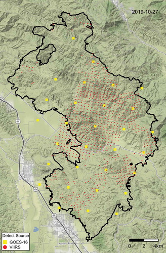
The disadvantage of thermal anomaly detection is that smaller and/or obscured fires (e.g., by clouds) will often be missed. A high percentage of prescribed fires are purposely designed to burn at low intensity and/or as understory burns; consequently, these are harder for satellites to detect (e.g., Nowell et al. 2018). That satellites miss a larger portion of prescribed fires compared to wildfires has been confirmed by comparisons with ground-based prescribed burning databases (Larkin et al. 2020; Larkin, Raffuse, and Strand 2014). Polar-orbiting satellites also need the fire to be active at the time of the satellite overpass, which may not correspond with the period of most active fire behavior. The Terra and Aqua polar-orbiting satellites have daytime overpass times of 10:30 am and 1:30 pm local time, generally ahead of the peak fire energetics that occur later in the afternoon when temperatures are higher, relative humidities are lower, and the mixed layer is more fully developed. Overpass timing can cause even larger fires to be missed if they are short in duration, a problem typical of quick-burning fuels such as grasslands. Geostationary satellites have the advantage of near-continuous daytime coverage, but, due in part to their higher orbits, the resolution (pixel size) reflects larger ground areas compared to polar-orbiting systems, thereby limiting their detection capabilities. Figure 4 shows an example of how different satellite systems can see the same fire, showing the GOES-16 and VIIRS hotspot detections for one day of the 2019 Kincade fire in California.

Figure 4. Satellite detections of the Kincade fire in northern California on October 27, 2019 by Geostationary Orbiting Environmental Satellite (GOES) and the polar-orbiting Visible Infrared Imaging Radiometer Suite (VIIRS). Hotspot detections by each are shown at the center points of the sensor pixels (yellow squares: GOES-16; red circles: VIIRS). Black outline: final fire perimeter. The VIIRS detections provide a higher resolution detection (~375 m), but only during overpasses. The geostationary GOES-16 provides a continuous observation but at a lower resolution (~2 km). The size of squares and circles is illustrative and not related to hotspot detection strength or size. Data sources: GOES and VIIRS detections based on NOAA Hazard Mapping System–collected detections; perimeter based on GeoMac data. Image source: U.S. Forest Service.

The NOAA Hazard Mapping System (HMS; NOAA, 2019; Ruminski et al. 2006; Schroeder et al. 2008) is an operational system that aggregates fire and smoke information from across various satellite systems and does quality control to remove identified false detections. Additionally, obscured fires that are not detected are added back in where visible imagery allows for geolocating the source of the plume. HMS fire detections are gridded onto a 1-km grid and are commonly used in smoke forecasting systems (O’Neill et al. 2008).

Burned area also can be detected by comparing satellite imagery on successive passes and identifying areas of vegetative change that are likely due to fire. This is typically done using LANDSAT (Tucker, Grant, and Dykstra 2004), AVHRR, or MODIS imagery. The result is an overall burned area or burn scar estimation (e.g., Kasischke and French 1995; Koutsias and Karteris 1998; Roy et al. 1999). Active hotspot detection can also be folded into the burn scar estimation (Giglio et al. 2009). The amount of change between overpasses at a given pixel reflects the change in biomass due to the fire. This measure is used by the U.S. Forest Service Monitoring Trends in Burn Severity (Eidenshink et al. 2007) project. Although such systems can provide highly detailed maps of specific burns, the process is generally applied only to larger burns, and in specific cases it can also have issues such as extremely large or small area estimations (e.g., Drury et al. 2014). The largest limitation for air quality purposes, however, is that such systems are based on 8-day LANDSAT 30-m resolution imagery, and so are too delayed for air quality forecasting purposes. MODIS-based products are available faster but with lower resolution (approximate 1-km resolution).

Satellite air quality measurements

Satellites provide a number of measurements relevant to air quality (Kahn 2020). The simplest is smoke extent polygons, such as those created operationally by the NOAA HMS (Ruminski et al. 2006; Schroeder et al. 2008). HMS smoke plumes extents are often used as a marker of being in a smoke plume but do not necessarily represent ground smoke impacts (Buysse et al. 2019; Kaulfus et al. 2017). For example, Figure 5 shows the HMS plumes extents for 11/8/2018 for the Camp wildfire (left panel) and surface measurements of 1-hr average PM_2.5 concentrations overlaid with the visible smoke plume from GOES-16 (right panel). Note that HMS vertically integrated smoke plumes extents may not represent ground-level concentrations: good air quality conditions at the surface (i.e., green) are present in some locations under the thickest visible smoke. Conversely, many monitors show poor air quality conditions (i.e., red) at locations where the visible satellite plume is much less dense. This comparison highlights how the satellite top-down view of the earth may not represent what we experience at the surface. Buysse et al. (2019), for example, found that surface PM_2.5 was enhanced on 30–80% of days with overhead HMS smoke plumes across 18 western U.S. cities. Locations closer to fire sources are more likely to have ground impacts when inside an identified smoke plume perimeter. In this way, satellite-derived smoke plume extent is a weak marker of ground impacts. However, the shape of the HMS plumes can be used to connect identified impacts back to fire sources (e.g., Brey et al. 2018) and to validate smoke forecasts (Rolph et al. 2009).

Figure 5. Camp wildfire, northern California, November 8, 2018. A NOAA HMS smoke plume at 12:30:00 PST. Colors are qualitative representation of smoke intensity (green: light, yellow: medium, red: heavy). (b) Visible satellite imagery from GOES-16 overlaid with surface measurements of 1-hr average PM_2.5 concentrations at 13:02:00 PST. Colors for the PM_2.5 data are associated with the AQI scale (see Figure 1). The right figure is from the NOAA Aerosol Watch program (https://www.star.nesdis.noaa.gov/smcd/spb/aq/AerosolWatch/).

Other smoke characteristics are available from satellites (e.g., Paugam et al. 2016). Plume top height is available from the Multi-angle Imaging SpectroRadiometer (MISR; Diner et al. 1998) instrument aboard the NASA polar-orbiting Earth Observing System (EOS) Terra satellite. MISR uses stereographic imagery to calculate plume top height. This system has been used to identify and evaluate overall fire plume top heights (Val Martin, Kahn, and Tosca 2018) since 1999 and provides the longest history of satellite-observed plume heights. Beyond providing plume top measurements, the vertical structure of plumes can be measured with the Cloud-Aerosol Lidar with Orthogonal Polarization (CALIOP; Hunt et al. 2009) satellite LiDAR system on the NASA Cloud-Aerosol Lidar and Infrared Pathfinder Satellite Observations (CALIPSO) satellite, launched in 2006. With the downward-facing LiDAR, CALIOP provides a vertically allocated measure of backscattering along the track of the satellite. Where this intersects smoke plumes, it can provide measures of the aerosol both at ground level as well as throughout the vertically sampled plume (Liu et al. 2009). Both MISR and CALIOP data have been used to examine plume rise models (e.g., Kahn et al. 2008; Raffuse et al. 2012; Val Martin et al. 2012; Val Martin, Kahn, and Tosca 2018), with modeled plumes showing generally consistent trends compared to the satellites, but with a large amount of variability.

Limitations of the use of these data to constrain modeled smoke plumes include both the timing of the overpass of the fire for MISR and the paucity of the number of times CALIOP, which is not a scanning instrument, intersects major plumes. MISR overpass times are typically in the mid-morning over the continental U.S., but fire plumes continue to grow into the afternoon when humidity, temperature, and development of atmospheric boundary layer typically lead to the highest plume heights. For CALIOP, Raffuse et al. (2012) found only 157 CALIPSO orbit paths (out of 25,000 orbits) intersecting HMS smoke plumes during a three-year period. The recent launch in 2017 of the TROPOspheric Monitoring Instrument (TROPOMI; Veefkind et al. 2012) on the European Space Agency sun-synchronous orbiting (similar to polar-orbiting) Sentinel-5 Precursor satellite, with its Aerosol Layer Height-derived product, offers the potential for daily global coverage and fast retrieval, and examination of this product has only recently started (Griffin et al. 2019). Additionally, Lyapustin et al. (2019) have recently derived a new methodology for determining plume injection height based on thermal differences of the rising plume with the surrounding air based on MODIS observations. Their algorithm is part of the Multi-Angle Implementation of Atmospheric Correction (MAIAC) MODIS collection six products, available daily at a 1-km resolution.

Aerosol optical depth (AOD) is a measure of the integrated amount of aerosol within the full vertical column of the atmosphere, derived from an estimation of the column-integrated attenuation of light due to scattering and absorption. AOD is available from both the polar-orbiting MODIS, the geostationary GOES, and the sun-synchronous TROPOMI. AOD is also available from VIIRS, where it is called aerosol optical thickness. AOD is useful for showing overall plume extent from major wildfires and, despite being column-integrated, statistical connections with ground-based AERONET measurements and others have allowed for the estimation of surface PM_2.5 from AOD (Drury et al. 2010; Gupta and Christopher 2009; Hu et al. 2014; Liu et al. 2005a; van Donkelaar, Martin, and Park 2006; Xie et al. 2015).

In addition to aerosols, satellites can detect other atmospheric components that can be used to track smoke plumes, including CO and NO₂. The Measurements of Pollution in The Troposphere (MOPITT) instrument onboard the Terra satellite, launched in 1999, measures column-integrated CO through the use of an array of specific wavelength channels where CO absorbs (Drummond et al. 2010). However, the instrument has non-uniform vertical sensitivity, complicating application and interpretation. Nonetheless, the result is the ability to record column-integrated CO levels across a substantial fraction of the planet each day. MOPITT data have been used to track smoke plumes over large areas (e.g., Lamarque et al. 2003; Liu et al. 2005b; Pfister et al. 2005). TROPOMI (on the Copernicus Sentinel-5 Precursor satellite) also measures CO, as well as CH₄, NO₂, SO₂, and other aerosol properties (Veefkind et al. 2012). Observations from OMI (on the NASA Aura satellite) have been used to understand NO₂ emissions from biomass burning (Mebust et al. 2011; Tanimoto et al. 2015). The upcoming Tropospheric Emissions: Monitoring of Pollution (TEMPO; Zoogman et al. 2014) geostationary mission is designed to augment and enhance current satellite capabilities for measuring atmospheric composition, and it will include a wide array of species, including O₃, NO₂, SO₂, and various aerosol properties of smoke plumes. By combining ultraviolet and visible wavelengths, TEMPO will, for the first time, allow satellite measurement of lower tropospheric (0–2 km altitude), free tropospheric, and stratospheric O₃. TEMPO also offers the promise of observing near-surface O₃, PM_2.5, and other pollutants at a higher resolution (e.g., 4.4 km x 2.1 km).

Field campaigns

Smoke has received increasing scrutiny from the atmospheric sciences and chemistry community via a number of large field campaigns that include ground-based, airborne, and satellite observations. These include the Department of Energy–sponsored Biomass Burning Observation Project (BBOP) campaign (https://www.arm.gov/research/campaigns/aaf2013bbop) (Briggs et al. 2016; Collier et al. 2016; Zhou et al. 2017), Studies of Emissions and Atmospheric Composition, Clouds and Climate Coupling by Regional Surveys (SEAC4RS) project (Toon et al. 2016), the NOAA-NASA Fire Influence on Regional to Global Environments and Air Quality (FIREX-AQ) campaign (https://www.esrl.noaa.gov/csd/projects/firex-aq/), the NSF-sponsored Western Wildfire Experiment for Cloud Chemistry, Aerosol. Absorption and Nitrogen (WE-CAN) campaign (https://www.eol.ucar.edu/field_projects/we-can), and the U.S. Department of Agriculture–sponsored Fire and Smoke Model Evaluation Experiment (FASMEE) experiment (https://sites.google.com/firenet.gov/fasmee/) (Prichard et al. 2019b). As of early 2020, much of this research has yet to be published, but as this work becomes available we anticipate many new findings and advances in the field, particularly in the areas of better estimations and models of emissions, speciation within smoke, and how smoke chemically ages and interacts with other pollutants in the air throughout the plume.

Emissions

Emissions from wildfires and prescribed fires in 2017

2017 was a major fire year; wildfires burned over 4 million hectares and prescribed fires almost 5 million ha. Tables 1 and 2 show the top five states for annual areas burned in 2017 for wildfires (Table 1) and prescribed fires (Table 2), along with some of the highest monthly areas burned for each state. The tables also show the PM_2.5 emissions for those months and the maximum observed daily mean PM_2.5 concentrations at any regulatory monitor for the month.

Table 1. Top five states for annual area burned as wildfires, from the EPA draft National emissions inventory for 2017. Also shown are the peak monthly areas burned (blue shading), peak monthly PM_2.5 emitted (orange), and the maximum PM_2.5 concentration measured at any regulatory monitor for the month (green; data from AirNowTech).

State	Annual Area Burned (ha)	Month	Month Area Burned (ha)	Month PM2.5 Emitted (tons)	Maximum Daily PM2.5 Measured in the Month (µg/m^3 24-hr avg)
California	641,440	August October	93,388 151,492	126,331 106,657	310 215
Montana	584,527	September	222,497	158,647	550
Nevada	519,250	July	373,169	21,742	135
Oregon	381,294	August	152,505	142,845	314
Idaho	367,205	August September	129,799 80,922	51,974 93,048	125 361

Table 2. Top five states for annual area burned as prescribed fires, from the EPA draft National Emissions Inventory for 2017. Also shown are the peak monthly areas burned (blue shading), peak monthly PM_2.5 emitted (orange), and maximum PM_2.5 concentration measured at any regulatory monitor for the month (green; data from AirNowTech).

State	Annual Area Burned (ha)	Month	Month Area Burned (ha)	Month PM2.5 Emitted (tons)	Maximum Daily PM2.5 Measured in the Month (µg/m^3, 24-hr avg)
Texas	632,470	February	143,468	12,807	29
Georgia	465,219	February	92,595	10,217	32
Oklahoma	449,616	March	140,656	18,615	49
Florida	386,518	February	90,367	8,733	30
Alabama	366,899	March	66,059	8,344	38

These tables convey several important results. First, area burned did not correspond to either PM_2.5 emissions or peak measured concentrations. Rather, the emissions depended strongly on fuel type and density as well as burning conditions. Compared to flaming combustion, smoldering fires emitted more PM_2.5 per unit of fuel consumed. Heavily forested regions, such as northern California and the Pacific Northwest, had much higher fuel loadings than rangelands (e.g., Nevada) and consequently much higher PM_2.5 emissions.

Second, even where PM_2.5 emissions were large, air quality monitors may not have measured high concentrations. This depended on the location of the fires relative to the monitors and transport. For example, the highest wildfire emissions in California were in August, and although the measured PM_2.5 concentration of 310 µg/m³ is notable, some state and USFS mobile monitors in several parts of the state reported even higher values on some days. The highest daily mean observed PM_2.5 in August at a non-regulatory monitor was 745 µg/m3 for a site near Happy Camp, CA, on 8/24/2017. (See https://wildlandfiresmoke.net for near-real time data access. Note that past non-regulatory data is not routinely made available. Contact the authors for more information about accessing this data.) In October, large areas burned in the Napa Wine Country fires. Although the emissions were somewhat lower compared to August, a large population was exposed to unhealthy to very unhealthy levels of PM_2.5 across the San Francisco Bay area (>200 µg/m³). These data show the clear signature of wildfires dominating the western U.S. in the summer months and into late fall in California.

In the central and southeastern U.S. (Table 2), prescribed burning peaks in late winter and spring. Although the area burned by prescribed fires was of a similar magnitude as wildfires in the West, the PM_2.5 emissions were approximately an order of magnitude lower, and the levels of measured PM_2.5 concentrations were also much lower. This difference is due to both the fuel types (e.g., rangelands) and the management practices in forest systems, where prescribed fires typically do not burn canopy or duff fuels. Thus, these data show that prescribed burning in the southeastern U.S. had much lower emissions per ha, likely due to the fuels and management goals for each fire.

The relationship between fire activity and smoke, 2004–2018

The relationship between the amount of fire in a region and human exposure to PM_2.5, O₃, and other pollutants is complex. Generally, increases in regional fire result in reduced air quality due to smoke, but this relationship is complicated by smoke transport from other regions and the locations of the fires with respect to in-situ air quality monitors. Figures 6 and 7 show the percentage of monitor-days that exceeded a daily average of 35 µg/m³ as well as the area burned in 2004–2018 for two states, California and Washington. California (Figure 6) showed a general trend to fewer days over 35 µg/m^3, due to decreasing industrial emissions (McClure and Jaffe 2018), but this number of days clearly increased with the high area burned in 2007, 2008, 2017, and 2018. If the temporal trend is removed, there is a significant correlation between area burned in California and the percentage of monitor-days over 35 µg/m³ (R² = 0.54).

Figure 6. (Top) Box and whisker plots of all daily PM_2.5 concentrations by year for air quality monitors in California. The numbers at the top of the panel show the total number of monitor-days above the daily PM_2.5 standard (35 µg/m³). Colored horizontal lines show the six AQI cut points: Good, <12 µg/m³; Moderate, <35.4 µg/m³; Unhealthy for Sensitive Groups, <55.4 µg/m³; Unhealthy, <150.4 µg/m³; Very unhealthy, <250.4 µg/m³; Hazardous, >250 µg/m³ (see Figure 1 for color key). (Bottom) Annual area burned (left y-axis) and percentage of all monitor-days that exceeded the daily PM_2.5 standard (right y-axis). All PM_2.5 data from the EPA AQS system are included (regulatory and non-regulatory). Sources: Burned area for each state is from NIFC, and PM_2.5 data are from the EPA AQS database.

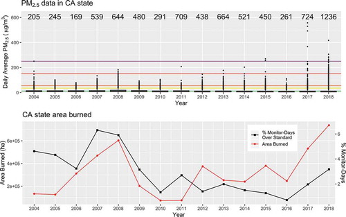
Figure 7. As in Figure 6, but for Washington.

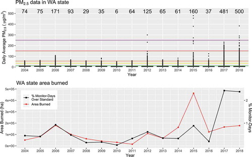
Washington (Figure 7) had fewer days over 35 µg/m³, but the frequency increased with the large area burned in 2006 and 2015. In 2017 and 2018, the percentage of days above 35 µg/m³ was much higher than in the previous decade, due not only to fires in Washington but also to transport of smoke from fires in Montana, British Columbia, and Oregon. This reflects the spatial pattern of fires and smoke and the spatial coverage of monitors within each state.

Emissions from fires

About 80–90% of the emissions by mass from biomass fires are of CO₂. Of the non-CO₂ portion, CO represents the largest fraction (~60%), followed by volatile organic compounds (VOC, ~15%), primary PM_2.5 (~8%), and CH₄ (~2%) (Akagi et al. 2011; Andreae 2019). Other gas phase emissions include inorganic species, including NOx, HCN, NH₃, and HONO. To date, more than 500 individual VOCs have been identified in smoke (Hatch et al. 2017), and these compounds are highly reactive with the OH radical (Kumar, Chandra, and Sinha 2018). Although VOCs represent only a fraction of the total gaseous emissions from biomass fires, many are associated with adverse health effects, and the mixture is more reactive than typical industrial emissions, with a high potential for secondary organic aerosol (SOA) and O₃ formation.

Primary smoke PM_2.5 emissions are composed mainly of organic compounds (>90%), with lesser amounts of elemental carbon (ca 5–10% by mass), NO₃⁻, K⁺, Cl⁻, NH₄⁺, and other constituents (Kondo et al. 2011; Liu et al. 2017b; Park et al. 2003; Zhou et al. 2017). Despite their much lower emissions compared to the organic compounds, these and other trace-level elements can be important for biogeochemical cycles and as tracers for source apportionment. For example, fires emit fluorine in globally significant amounts (Jayarathne et al. 2014). Smoke particles are mostly small, with median diameters in the range of 50–200 nm (Carrico et al. 2016; Laing, Jaffe, and Hee 2016), although a few larger particles can extend into the super micron range (e.g., Maudlin et al. 2015). The emissions are variable from fire to fire and depend on fuel type, fuel moisture, fire conditions, temperature, weather, and other factors (Cubison et al. 2011; Hecobian et al. 2011). This variability is a major challenge for understanding the emissions, chemistry, and subsequent impacts of smoke.

Emissions inventories

An emissions inventory (EI) provides a detailed accounting of hectares burned and the pollutants emitted from each fire. An EI is typically used both as an input for air quality models and health assessments and to gauge the relative amounts of different pollutants emitted to the atmosphere. Emissions of species x is often calculated from:

(1) $E_x=A\times B\times FB\times E{F}_x$(1)

Where E_x is the mass of species x emitted, A is the area burned, B is the mass of biomass per unit area, FB is the fraction of biomass consumed, and EF_x is the emission factor per unit fuel consumed for species x (Seiler and Crutzen 1980; Urbanski 2014; Wiedinmyer et al. 2011).

North America has two national EIs: the EPA’s NEI (U.S. EPA, 2019a) and the Canadian Air Pollutant Emissions Inventory (APEI; Canada, 2019). At a global scale, there are several EIs for fire emissions, including the Fire Inventory from National Center for Atmospheric Research (FINN; Wiedinmyer et al. 2011), the Global Fire Emissions Database (GFED; van der Werf et al. 2017), the Global Fire Assimilation System (GFAS; Kaiser et al. 2012), and the Integrated System for wild-land Fires (IS4FIRES; Soares, Sofiev, and Hakkarainen 2015).

Unlike the other EIs, which rely solely on satellite fire detects, the NEI uses fire activity data obtained from national, regional, and state reporting (e.g., federal incident reports used to calculate National Interagency Fire Center [NIFC] statistics, Fire Emissions Tracking System [FETS, htto://wrapfets.org]), augmented and reconciled with satellite data (e.g., from NOAA’s Hazard Mapping System) (Larkin et al. 2020). The BlueSky emissions modeling framework (Larkin et al. 2009) is then used to generate daily fire emissions, and the EPA applies PM chemical speciation, vertical allocation, and a temporal profile according to the fire type: agricultural, prescribed fire, or wildfire and by season and location (Eyth et al. 2019; Pouliot et al. 2017).

EIs developed from activity reports require considerable effort to develop and are reported retrospectively on a temporally resolved annual (e.g., Canada’s APEI) or triennial basis (e.g., NEI); in contrast, EIs based solely on satellite detection can, in principle, be reported in near-real time. Between NEI years, the EPA also develops fire emissions for air quality modeling purposes, using the same data sources but without the extensive review process done for the NEI (Koplitz et al. 2018). By consolidating multiple sources for fire activity, the NEI hectares burned are nearly 20% higher than NIFC–reported wildfire areas and over 100% higher than GFED burned areas, likely due to the inclusion of smaller prescribed fires that may not be reported to NIFC or detected by satellite (Larkin et al. 2020). Emissions can also be estimated by applying smoke emission coefficients to fire radiative power (FRP), avoiding some of the uncertainty in fuel loading and amount consumed (e.g., the NASA Fire Energetics and Emissions Research algorithm; Ichoku and Ellison 2014). However, this approach can miss low-intensity, short-duration, understory fires, resulting in a 54% lower PM_2.5 emission estimate compared to the NEI (Li et al. 2019a). Comparisons among EIs and the NEI are still sparse.

Emission factors

Emission factors (EFs; see equations 1 and 2) are a critical input parameter in wildland fire EIs and emissions models (e.g., BlueSky Modeling Framework; Larkin et al. 2009). EFs are defined as a mass of species emitted per unit mass of dry fuel consumed (Andreae 2019). The carbon balance method (Radke et al. 1988; Ward et al. 1982) is the most widely used approach to calculate EFs:

(2) $E{F}_x=F_c\frac{\mathrm{\Delta }{C}_x}{\sum _i\mathrm{\Delta }{C}_i}$(2)

Where EF_x is the EF of species x, F_c is the fraction of carbon in the fuel, ΔC_x is the excess carbon mass concentration of species x (often concentrations are replaced with normalized excess emissions ratio to CO₂ or CO), and the denominator is the sum of the carbon from all carbon-containing species, often limited to CO₂ and CO. The carbon balance method has several assumptions that may introduce error into the EF calculation:

1. All carbon in the burned fuel is consumed – Carbon remaining in the fuel as char is frequently omitted in the carbon balance, which results, on average, in a 4% overestimate (Surawski et al. 2016).

2. All major carbon-containing species emitted are accounted for – CO₂ and CO typically account for ~96% of the carbon emissions (Yokelson et al. 1999); ignoring VOCs and particulate carbon results in an overestimate in EFs of about 4%.

3. Carbon fraction of the fuel is known and approximately constant – Carbon fractions of 0.45–0.50 (Andreae 2019; Yokelson et al. 1999) are commonly used when fuel-specific information is not known, increasing uncertainty in the EF about 10% (Susott et al. 1996).

4. All species are transported to the measurement location with no losses or deposition – The effect of this assumption is unknown (Hsieh, Bugna, and Robertson 2016).

5. Background concentrations are accurately accounted for – Background CO₂ enhancement in dilution air underestimates the EFs by about 6% (Hsieh, Bugna, and Robertson 2016). Aircraft measurements downwind encountering background air masses of varying pollutant levels (e.g., at boundary layer vs. free troposphere) can result in a large (>50%) change in normalized excess emission ratios (Chatfield et al. 2019; Yokelson, Andreae, and Akagi 2013). Briggs et al. 2016, see supplemental information) propose a method to compute the uncertainty in these values due to this effect.

These assumptions introduce a positive bias, with added uncertainty from approximating a constant carbon fraction in the fuel. These errors are outside measurement errors, which for some species, like PM, may be sizable as well. However, the uncertainties in the measurement and calculation of EFs are eclipsed by the immense variability of emissions from varying fuels and combustion conditions, as evidenced by the wide range of EFs reported in the literature. Note that the EF equation is similar to one used for enhancement ratios (ERs), but EFs are reserved for cases where fire emissions are observed directly, and ERs are used for downstream measurements, where significant processing of the emissions may have occurred (e.g., Briggs et al. 2016).

The large variability in EFs has been a major driver of research on the emissions from wildland fires. Over the past two decades, a number of EF compilations have been published for global wildland fires and other types of biomass fires (e.g., charcoal making, home biofuel, trash burning; Akagi et al. 2011; Amaral et al. 2016; Andreae 2019; Andreae and Merlet 2001). Other EF compilations have focused on North American wildland fires including wild and prescribed fires (e.g., Lincoln et al. 2014; Prichard et al. 2020; U.S. EPA, 1995; Urbanski 2014; Ward et al. 1989). New emissions studies investigating different fuels, fire types, and emissions characteristics are published frequently, which is why some compilations provide periodic updates. The FINN emission factor compilation is periodically updated with emission factors from recently published studies (http://bai.acom.ucar.edu/Data/fire/). Prichard et al. (2020) developed the Smoke Emissions Reference Application (SERA; https://depts.washington.edu/nwfire/sera/index.php) to be a searchable online EF repository.

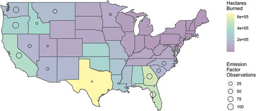
Compiling EFs into a cohesive database also facilitates the assessment of data gaps for fuel types/ecoregions, combustion conditions, and pollutants, and it provides a tool for understanding how emissions vary with these parameters. Comparing the EF observations with the average hectares burned in each state from 2006 to 2016 (U.S. EPA, 2019a) reveals that some areas of the U.S. with high fire activity are overlooked in emissions studies (Figure 8). For example, Texas, which has the highest average burned area in the country, has only two EF observations in the SERA database. Other central and southern U.S. states also have high areas burned but few or no EFs in SERA. This limits our understanding of the impact of these fires on air quality.

Figure 8. Comparison of the annual average hectares burned for each state in the continental U.S. (2006–2016) with the number of particulate matter emission factor observations for each state in the SERA database.

Of the major species in SERA, 75–90% of the EFs are from laboratory studies, 10–20% are from prescribed fires, and <5% are from wildfires. The exception is for CO₂ and CO, for which there are ~600 observations, with approximately 15% fromwildfires and the remaining EFs evenly split between lab and prescribed fires. Other pollutants, like NOx, NH₃, or some of the more commonly measured VOCs, like CH₄, have only around 200 EFs across all fuel and ecosystem types (Table 3).

Table 3. Comparison of average emission factors (EFs) from non-biomass fuels (e.g., structures, furnishings, vehicles) at the wildland-urban interface (WUI) and from natural fuels from wildland fires, derived from SERA. EF units are g/kg fuel consumed, unless otherwise noted.

	CO2	CO	HCN	NOx	HCl	SO2	PM	C6H6	Benzo(a) pyrene	Polychlorinated dibenzo-p-dioxins (µg/kg)	Polychlorinated dibenzofurans (µg/kg)
Average EF for non-biomass WUI fuels	1514	124	8.8	5.7	153	62.2	66.7	31.4	0.12	0.53	14.0
# EFs observed	143	145	49	21	32	14	97	41	18	4	4
Standard deviation	917	130	41.6	19.4	404	164	84.9	67.2	0.19	1.04	28.0
Average EF for wildland fires	1550	104	0.5	2.2	0.3	1.1	25.1	0.4	0.0003	0.032	0.021
# EFs observed	597	640	188	202	37	125	688	84	11	13	13
Standard deviation	313	58	0.6	2.1	0.9	0.7	34.8	0.3	0.0002	0.020	0.017
WUI/wildland fire EF ratio	0.98	1.2	19	2.6	488	56	2.7	85	366	16	667

Historically, wildland fire emissions have been modeled using the two basic combustion phases: flaming or smoldering (Prichard, Ottmar, and Anderson 2007). The modified combustion efficiency (MCE) is used as the primary indicator of combustion phase, with MCE > 0.9 considered flaming combustion and MCE < 0.9 as smoldering combustion (Urbanski 2014). MCE is defined as:

(3) $MCE=\frac{\mathrm{\Delta }C{O}_2}{\mathrm{\Delta }C{O}_2+\mathrm{\Delta }CO}$(3)

Where ΔCO₂ is the excess CO₂ concentration and ΔCO is the excess CO concentration. EFs for pollutants associated with incomplete combustion (CO, CH₄, and PM) are all moderately to strongly correlated with MCE (r² = 0.64, 0.71, and 0.47, respectively; Prichard et al. 2020). Some compounds, like NOx, are poorly predicted by MCE (r² = 0.07; Prichard et al. 2020) but have been found to be linearly correlated with fuel nitrogen (Delmas, Lacaux, and Brocard 1995). Elements such as K, Cl, and Ca also appear; these can vary widely among fuel types and depend more on fuel composition, with combustion conditions playing a secondary role.

Prichard et al. (2020) analyzed the SERA EF database to identify conditions with few EF observations. More information is still needed for wildfire EFs, particularly because some studies indicate much higher wildfire EFs, possibly due to the greater consumption of coarse wood, duff, and moist canopy fuels (Liu et al. 2017a). There is also a need for more EFs for smoldering conditions, especially from coarse wood and duff fuel types. Information is limited on how the environmental conditions and the fire behavior affect emissions, which are important considerations for prescribed fire burn plans (Waldrop and Goodrick 2012). The observations on prescribed fires also presents contradictory results. Bian et al. (2020) reported that prescribed fires in the southeastern U.S. tend toward more‐smoldering conditions compared to other parts of the country, which would presumably increase the PM_2.5 EFs (Prichard et al. 2020). But Liu et al. (2017a) reported lower PM_2.5 EFs from southeastern prescribed fires compared to western wildfires. A better understanding of the factors and environmental controls associated with prescribed burning is needed to improve our estimates of their emissions.

Primary gas phase emissions

Gas phase emissions are composed of oxidized species associated with flaming conditions, including CO₂, NOx, HONO, SO₂, and more reduced species associated with smoldering conditions, including CO, CH₄, HCN, and NH₃. Both combustion phases are associated with emissions of VOCs, and these have a range of volatilities, oxygenation, heteroatoms (N, F, S, Cl, Br, I), and functional groups (e.g., ketones, carbonyls, alcohols) (Prichard et al. 2020). Most of the VOCs are unsaturated compounds (>80%), and around 60% are oxygenated-VOCs (OVOCs) (Gilman et al. 2015). The most abundant OVOCs emitted from typical U.S. fuels are formaldehyde, formic acid, methanol, acetaldehyde, and acetic acid. Levoglucosan and phenolic compounds (e.g., cresols, guaiacol) are also nearly ubiquitous, but in highly variable amounts (Hatch et al. 2018). Most VOCs vary greatly in their relative abundance across different fuels, and some are unique to specific fuel types (Hatch et al. 2018), demonstrating the difficulties of attempts to simplify emissions models for even the most commonly emitted molecules.

Many of the VOCs correlate only modestly with MCE and are better categorized as products of the initial distillation of fuel or from low or high temperature pyrolysis reaction pathways (Sekimoto et al. 2018). During the brief initial distillation phase, the higher volatility of unburned fuel compounds, like monoterpenes and other biogenic-derived VOCs, are emitted (Sekimoto et al. 2018). Despite contributing minimally to the overall VOC emissions, these biogenic VOCs may have an important role in flammability, by reducing ignition times (De Lillis, Bianco, and Loreto 2009; Owens et al. 1998) and enhancing the rate of fire spread (Chetehouna et al. 2014). The low-temperature pyrolysis products include a greater fraction of low volatility compounds, oxygenates, furans, and ammonia, while the high-temperature products have few low-volatility compounds and are enriched in aliphatic hydrocarbons, PAHs, HCN, HCNO, and HONO (Sekimoto et al. 2018).

Primary particle emissions – chemical, physical, and optical characteristics

Particle emissions from wildland fires are complex, with time-varying size, morphology, chemical composition, and volatility, all of which determine their impact on human health and the environment. PM emissions are composed mainly of organic carbon (50–75%), with 5–10% elemental carbon (EC) or black carbon (BC), and typically less than 5% of inorganic ions (e.g., K, Cl) and metals (Ward and Hardy 1988); the balance of the PM mass is from elements associated with organic carbon (e.g., H, O, N, S). Note that EC and BC are not equivalent and depend on the measurement methodology (Andreae 2019; Petzold et al. 2013). Measurements of complete particle composition are still relatively sparse (Balachandran et al. 2013; Einfeld, Ward, and Hardy 1991; Lee et al. 2005; Ward and Hardy 1988), with many not reporting either the organic fractions (Alves et al. 2019, 2011; Reisen et al. 2018) or the inorganic fractions (Aurell and Gullett 2013; Aurell, Gullett, and Tabor 2015; Holder et al. 2016; Vicente et al. 2013). Toxic metals are also present in PM at very low levels (Alves et al. 2011; Gaudichet et al. 1995; Popovicheva et al. 2016), but they may be enriched in emissions from wildland fires that occur on or near contaminated sites (Kristensen and Taylor 2012; Odigie and Flegal 2014; Wu, Taylor, and Handley 2017).

Organic emissions have a range of volatilities (gas phase, intermediate volatility, semivolatile, low volatility, particle phase), which makes measuring PM difficult, because up to 40% of the PM mass may be lost due to evaporation of the semivolatile compounds (Hatch et al. 2018). The distribution across the volatility range is relatively constant for most combustion conditions and fuels (May et al. 2013). The lowest-volatility fraction consists primarily of anhydrosugars, whereas alcohols and acids dominate the semivolatile range, and phenols dominate in the higher volatility range (Hatch et al. 2018).

Most lab and field studies have demonstrated that BC emissions increase with MCE (e.g., Jen et al. 2019; Selimovic et al. 2018), but other studies have found a weaker relationship (e.g., Hosseini et al. 2013; McMeeking et al. 2009). Laboratory burning studies have suggested larger BC particle mass fractions compared to field observations under flaming conditions (lab: 15 ± 12%, field: 8 ± 5%) as well as higher inorganic content (lab: 12 ± 13%, field: 8 ± 5%) (Alves et al. 2011; Balachandran et al. 2013; Ferek et al. 1998; Guo et al. 2018; Hosseini et al. 2013; McMeeking et al. 2009; Turn et al. 1997; Ward and Hardy 1988). Both results suggest that laboratory burning cannot fully capture the characteristics of wildland fire emissions.

The composition of PM affects its size, morphology, and hygroscopicity, all of which impact optical properties. The BC fraction is formed during flaming combustion; it is composed of graphitic-like primary particles, with diameters of 20–50 nm that aggregate into larger particles of approximately 200 nm (volume equivalent diameter) (Holder et al. 2016; Sahu et al. 2012; Schwarz et al. 2008) that are hydrophobic (Petters et al. 2009). However, most PM is organic with moderate hygroscopicity (Petters et al. 2009) and, for fresh emissions, has a single size mode with count median diameters (CMD) of ~120 nm and geometric standard deviations (GSD) of ~1.7 (Janhäll, Andreae, and Pöschl 2010; Reid et al. 2005; Virkkula et al. 2014; Wardoyo et al. 2007). Some fuels, like grasses and some shrubs, emit PM with a larger inorganic fraction, resulting in larger hygroscopicity (Carrico et al. 2010; Petters et al. 2009) that may impact light-scattering properties of biomass burning aerosols at high relative humidities (Gomez et al. 2018). Aging causes the PM to converge to a moderate hygroscopicity, likely due to secondary organic aerosol formation (Engelhart et al. 2012; Lathem et al. 2013), making these particles able to serve as cloud condensation nuclei under some conditions. Aging also results in larger particles but with a narrowed size distribution, with CMDs around 175–300 nm and GSDs of 1.3–1.7 (Janhäll, Andreae, and Pöschl 2010); however, wide ranges of CMDs and GSDs have been observed in plumes of various ages and transport histories (Laing, Jaffe, and Hee 2016). PM from flaming emissions are mostly larger than those from smoldering (Janhäll, Andreae, and Pöschl 2010), but mixed results have been seen in the lab from the same fuel (Ordou and Agranovski 2019), and some smoldering fires produce larger particles (Iinuma et al. 2007). PM (both the OC and BC fraction) from grassland fires tends to be smaller than PM from fires of forests or shrublands (Holder et al. 2016; Reid et al. 2005). More field measurements of size and composition of PM emissions from many types of fires and combustion conditions are needed.

Among the organic fraction, tar balls are another distinct particle type that as yet can be conclusively identified only through electron microscopy (Pósfai et al. 2004, 2003). Tar balls are characterized as highly viscous spherical particles (100–300 nm diameter) or aggregates thereof (Girotto et al. 2018; Hand et al. 2005; Pósfai et al. 2004), stable at high temperatures (retaining 70% of tar ball mass at 600 C; Adachi et al. 2019), and composed of amorphous carbon, oxygen, often sulfur, and trace levels of potassium (Adachi et al. 2019). How tar balls are formed is still uncertain (Hand et al. 2005; Sedlacek et al. 2018; Toth et al. 2018), but they appear to increase in number fraction with plume age (Adachi et al. 2019; Sedlacek et al. 2018). Tar ball optical properties and how they relate to other types of organic carbon have yet to be resolved.

Much recent research on smoke PM optical properties has focused on absorption due to the considerable uncertainty in the climate impacts of smoke from wildland fires (Jacobson 2014). Optical properties also affect rates of photolysis (Baylon et al. 2018; Mok et al. 2016) and photosynthesis (Hemes, Verfaillie, and Baldocchi 2020), and they are a critical factor in remote sensing of PM (Li et al. 2019b) and source identification (Schmeisser et al. 2017). Both the BC fraction and the organic fraction contribute to the absorption. BC absorbs across a broad wavelength range, with a weak variation characterized by an angstrom absorption exponent (AAE) of 1 (Bond and Bergstrom 2006). The angstrom absorption exponent is calculated by:

(4) $AAE=-\frac{lnabs({\lambda }_1)/lnabs({\lambda }_2)}{{\lambda }_1/{\lambda }_2}$(4)

Where abs is the absorption and λ is the wavelength. Some portion of the organic fraction has strong absorption in the UV wavelengths, with AAEs typically >2. This fraction is referred to as brown carbon (BrC) (Andreae and Gelencsér 2006) and is composed of organic compounds such as polycyclic aromatics, nitroaromatics, and humic-like substances (Laskin, Laskin, and Nizkorodov 2015). But rather than being two distinct PM types (BC and BrC), PM may exhibit a continuum of compositions, volatilities, and optical properties from BC to BrC (Adler et al. 2019; Saleh, Cheng, and Atwi 2018).

Emissions from fires in the wildland-urban interface (WUI)

In the wildland-urban interface (WUI), structures, vehicles, and the substances contained within them also burn and contribute to emissions. These “fuels” have very different chemical compositions from natural fuels (soils, grasses, shrubs, and trees) and likely very different emissions. A number of studies have measured emissions from structure and vehicle fires (e.g., Fabian et al. 2014, 2010; Fent et al. 2018; Lecocq et al. 2014). These have shown a wide array of harmful emissions, including irritants (HCl, HF, NO₂, HS, SO₂), asphyxiants (CO, HCN), sensitizers (Isocyanates), carcinogens (formaldehyde, benzene, PAHs, dioxins), and toxic metals (Cd, Cr, Pb). To our knowledge, no EI or model exists that includes emissions from structure or vehicle fires as part of the emissions from wildland fires. Several studies have reported EFs from building materials and furnishings, but few have measured emissions from full-scale fires (Blomqvist, Rosell, and Simonson 2004; Gann et al. 2010; Lönnermark and Blomqvist 2006; Wichmann, Lorenz, and Bahadir 1995). Most studies have measured emissions from small pieces of these materials combusted in a cone calorimeter or tube furnace. Of the studies with EFs, none provides a complete assessment of all such emissions that may impact human health or the environment, for example, inorganic gases (Blomqvist, Rosell, and Simonson 2004; Gann et al. 2010; Kozlowski, Wesolek, and Wladyka-Przybylak 1999; Lönnermark and Blomqvist 2006; Lönnermark et al. 1996; Persson and Simonson 1998; Stec and Hull 2011), PM (Blomqvist, Rosell, and Simonson 2004; Elomaa and Saharinen 1991; Fabian et al. 2010; Lemieux and Ryan 1993; Lönnermark and Blomqvist 2006; Reisen, Bhujel, and Leonard 2014; Valavanidis et al. 2008), VOCs (Blomqvist, Rosell, and Simonson 2004; Durlak et al. 1998; Font et al. 2003; Lemieux and Ryan 1993; Lönnermark and Blomqvist 2006; Lönnermark et al. 1996; Moltó, Font, and Conesa 2006; Reisen, Bhujel, and Leonard 2014), PAHs (Blomqvist et al. 2014; Blomqvist, Persson, and Simonson 2007; Blomqvist, Rosell, and Simonson 2004; Durlak et al. 1998; Elomaa and Saharinen 1991; Font et al. 2003; Lemieux and Ryan 1993; Lönnermark and Blomqvist 2006; Moltó, Font, and Conesa 2006; Reisen, Bhujel, and Leonard 2014; Valavanidis et al. 2008), dioxins (Blomqvist, Rosell, and Simonson 2004; Lönnermark and Blomqvist 2006), and toxic metals (Lemieux and Ryan 1993; Lönnermark and Blomqvist 2006; Valavanidis et al. 2008). Thus, extrapolation across studies is necessary to obtain a complete picture of emissions, which is needed, for example, to understand health impacts or to model fire chemistry for exceptional event demonstrations.

Table 3 compares the average EFs from the combustion of non-biomass WUI fuels (structures, vehicles, furnishings, and structural materials) and biomass fuels, derived from the SERA database. The EFs from the primary combustion products – CO₂, CO, and NOx – are similar for WUI and natural fuels. However, most WUI VOC EFs were far greater than those from natural fuels, with WUI/natural ratios ranging from 4 (propene) to over 2,000 (Diebenzo(a,h)anthracene). These EFs are highly variable, with relative standard deviations of 200–500%. In contrast, the EFs for aldehydes (formaldehyde, acetaldehyde, and acrolein) had much lower WUI/natural ratios (0.12–0.9). The large WUI/natural ratios for the most toxic compounds suggest that fires in the WUI may present a substantial hazard to firefighters and nearby communities, despite the far lower “fuel” consumption in the WUI. However, estimates of emissions including structures and vehicles are still needed to accurately determine the impacts of smoke from fires in the WUI. This variability and the uncertainty in emissions from an individual fire propagate into uncertainties in forecast air quality impacts.

Transport

Once emitted, gases and particles interact with, and modify, the atmosphere in terms of physical processes such as airflow, heating of surrounding atmosphere, and radiative properties. Emissions associated with flaming combustion typically get injected higher into the atmosphere than emissions associated with smoldering combustion. On a micro scale these processes occur individually, but on a macro scale they occur simultaneously as a fire progresses across the landscape. Computational fluid dynamic (CFD) systems such as the Wildland-urban interface Fire Dynamics Simulator (WFDS) (Mell et al. 2007, 2009; Mueller, Mell, and Simeoni 2014) and FIRETEC (Linn et al. 2002, 2005) explicitly simulate these physical processes, with a focus on simulating the detailed combustion and propagation of the fire.

During combustion, energy is released in the form of radiation and latent and sensible heat. Radiant heat is transferred through the atmosphere and is largely responsible for the preheating of fuels. Sensible heat, in the form of conduction and convention, heats the surrounding atmosphere. Latent heat from the condensation of water vapor in the plume releases additional energy. The combination of these processes is responsible for lofting fire emissions vertically into the atmosphere.

As the emissions are injected, the plume entrains cooler air and mixes with the surrounding environment. In one of few studies that provide insight into the entrainment structures in a wildfire convective plume, Lareau and Clements (2017) used lidar to measure how this entrainment dilutes and expands the plume as it rises. Fires are often composed of multiple plume updrafts (Achtemeier et al. 2011), which have smaller ascending velocities and are more affected by entrainment (Liu et al. 2010) than a single plume. The flaming front will also pull air in at its boundaries to fuel the combustion process. These phenomena represent the coupling of the fire with the atmosphere, which happens when the heat supplied by the fire is sufficient to overcome the kinetic energy of the ambient flow (Clements and Seto 2015) and results in modifications to the wind and temperature fields. Coupled fire-atmosphere modeling systems, such as the Weather Research and Forecasting (WRF) WRF-SFire (2014; Mandel, Beezley, and Kochanski 2011) and the Coupled Atmosphere-Wildland Fire-Environment (CAWFE) (Clark, Coen, and Latham 2004; Coen et al. 2013), compute fire spread using the Rothermel algorithm (Andrews 2018; Rothermel 1972), which is less computationally intense than the CFD approaches of WFDS and FIRETEC.

The plume injection height is controlled by the thermodynamic stability of the atmosphere and surface heat flux released from the fire (Freitas et al. 2007). The initial maximum height that the smoke plume reaches is referred to as the plume rise. Many methods have been developed to estimate this parameter, ranging from the traditional empirical approach by Briggs (1975), originally developed for power plant stack emissions, to 1-D models that include cloud microphysics and other boundary layer conditions (Freitas et al. 2007). Some methods rely upon radiant heat measured from space by remote-sensing instruments (Sofiev, Ermakova, and Vankevich 2012). Both ground-based and remote sensor-based studies have been conducted to evaluate various plume injection height schemes. Cunningham and Goodrick (2013) and Lareau and Clements (2017) found that their single plume measurement cases compared well to those of Briggs (1975). Raffuse et al. (2012), using data from the Multi-angle Imaging SpectroRadiometer (MISR) onboard the Terra satellite, found that the Briggs scheme was systematically low for smaller fires and high for large fires. Val Martin et al. (2012) evaluated parameterizations developed by Freitas et al. (2007) with MISR data and found that this approach tended to underestimate plume rise and did not perform well at identifying when plumes were injected into the free troposphere. Paugam et al. (2016) provide a comprehensive review of plume rise performance in chemical transport models along with the atmospheric and fire parameters governing plume rise.

An important corollary to plume injection height is the concept of how gases and aerosols are initially injected in the vertical, which is critical to atmospheric modeling of smoke plumes. The assumption is that emissions are distributed equally from either the ground to plume top or from an assumed plume bottom to the plume top. Mallia et al. (2018) found that model results were improved when fire emissions were distributed vertically below the plume top in a Gaussian manner. Systems such as the BlueSky Smoke Modeling Framework (Larkin et al. 2009) attempt to address this vertical allocation question by distributing smoldering emissions near the surface and flaming emissions aloft. Lidar data from both satellites and ground-based measurements can help track the vertical distribution of emissions (Banta et al. 1992; Clements et al. 2018; Lareau and Clements 2017). For example, Lareau and Clements (2017), in their measure of the turbulent structure of a plume using ground-based lidar, found a Gaussian distribution of backscatter (and thus smoke) in their single-plume study. Remotely sensed lidar data from the Cloud-Aerosol Lidar with Orthogonal Polarization (CALIOP) instrument gives vertical cross-sections of the atmosphere, and, if the swath occurs over a fire emission point, the data can inform the vertical injection distribution. The data also illustrate the stratification of smoke plumes – how layers may travel at different heights in the atmosphere, remain aloft, or mix at the surface. From downwind swath data, back-trajectory analyses using the methods of Soja et al. (2012) give information about the initial vertical distribution of emissions as well as contributions from multiple fires, if present.

Studies using MISR data found that emissions from most fires (>80%) are injected into the boundary layer, and the remaining smaller percentage of fires inject above the boundary layer (Paugam et al. 2016; Sofiev, Ermakova, and Vankevich 2012; Sofiev et al. 2009; Val Martin, Kahn, and Tosca 2018). Emissions emitted near the surface are subject to local and regional flow regimes (e.g., up-valley and down-valley drainage flows in complex terrain). Emissions injected above the atmospheric boundary layer, although fewer, have longer atmospheric lifetimes and are more available for long-range transport.

A special case where emissions are transported very high into the atmosphere is when large buoyant plumes develop cumulus clouds, releasing latent heat and further enhancing vertical transport. These pyrocumulus (pyroCu) clouds can, in rare cases, develop into thunderstorms, known as pyrocumulonimbus (pyroCb). PyroCb activity and buoyant plumes can inject gases and aerosols into the upper troposphere or lower stratosphere, where they can persist for weeks and months; these emissions can then be transported on a hemispheric scale (Fromm and Servranckx 2003; Fromm et al. 2006; Peterson et al. 2017; Sofiev, Ermakova, and Vankevich 2012). The exact mechanisms of pyroCb formation are still an active area of debate (Peterson et al. 2017) and research (Lareau and Clements 2016). Although pyroCb are a special subset of smoke plumes, the scope and scale of their emissions and the height of injection have been likened to that of a volcano, and a single event can reduce surface temperatures on a hemispheric scale. Fromm et al. (2010) suggest that some stratospheric aerosol layers previously assumed to be from volcanic eruptions were, in fact, due to pyroCb events.

Once emissions reach a point of neutral buoyancy, transport occurs similar to other atmospheric constituents. Diurnal processes, such as surface heating and cooling, along with regional winds, fronts, and topography, control smoke concentrations near the surface and within the mixed layer. Daytime heating of the surface creates an unstable boundary layer that can dilute smoke concentrations or entrain smoke aloft. At higher wind speeds, the atmosphere becomes more stable, which reduces vertical mixing. Smoke emitted in these conditions can be stratified, tending to transport within the layer it was emitted. As night approaches, the ground cools faster than the atmosphere, creating a near-surface stable layer. Smoke emitted at night near the ground will often stay near the ground. Smoke emitted earlier in the day will remain above in the middle portion of the nocturnal atmospheric boundary layer. In complex terrain such as mountain valleys, daytime heating will create up-valley winds, and then at night, surface cooling will cause the winds to shift and flow down valley (Whiteman 2000). Population centers are often located within valleys, and these nighttime down-valley flows can transport smoke into town, resulting in high concentrations, especially if fuels up valley continue to emit through the night (Miller et al. 2019). In the humid southeastern U.S., smoldering fire emissions along with the higher atmospheric water content (both emitted from the fire and the surrounding atmosphere) can form a thick fog with near-zero visibility conditions (Achtemeier 2006; Bartolome et al. 2019). This smoke can travel along fine-scale topographical depressions (Achtemeier 2005) and has been attributed to catastrophic vehicle collisions (Bartolome et al. 2019).

Smoke and the physical atmosphere are highly coupled. Smoke modifies the radiative properties of the atmosphere by blocking the sun from reaching the surface and absorbing heat and re-emitting that heat to the surrounding atmosphere. This increases atmospheric stability within the mixed layer, makes temperatures cooler near the surface, and reduces both the height of the mixed layer and mixing of smoke through the layer; it may reduce wind speeds as well. In theory, these processes will increase surface concentrations, although there is currently no experimental evidence of this. Absorption of solar radiation by the smoke will also delay the breakup of the nighttime stable layer, maintaining the subsidence inversion much later into the day.

Vant-Hull et al. (2005), Markowicz, Lisok, and Xian (2017), and McKendry et al. (2019) discussed these feedback mechanisms for North American cases. These phenomena have large implications for concentrations, transportation safety, and visibility. For example, during 2017 in the Willamette Valley in Oregon, stagnant air maintained high PM concentrations from nearby fires as lower wind speeds reduced smoke mixing and transport. Other unique examples are smoke-induced density currents that form from differential solar heating between smoke-filled and smoke-free portions of the atmospheric boundary layer. These density currents are relatively common near large wildfires. Lareau and Clements (2015) conducted the first measurements of these density currents, which can spread smoke counter to the ambient wind and over large distances (∼30 km), thereby contributing to rapid wind shifts, reductions in visibility, and delayed inversion breakup.

To properly account for these phenomena, the transport model needs to account for radiative effects on the meteorology due to the presence of smoke. Some examples of systems that do this are GEOS-Chem (Bey et al. 2001), WRF-Chem (Grell et al. 2005), and WRF-Community Multi-scale Air Quality (WRF-CMAQ) (Wong et al. 2012). Two operational implementations of these systems are the High Resolution Rapid Refresh (HRRR) forecasting system and recent work modifying the Northwest Regional Modeling Consortium WRF forecast system (Vaughan et al. 2004) to ingest GEOS-5 AOD to modify surface temperatures.

Special cases of transport that have large impacts on fire behavior and downwind air quality are Santa Ana winds (Kolden and Abatzoglou 2018; Langford, Pierce, and Schultz 2015; Mensing, Michaelsen, and Byrne 1999; Westerling et al. 2004), Diablo winds (Mass and Ovens 2019), and Sundowner winds (Blier 1998). Santa Ana winds are strong northeasterly winds with low relative humidity that occur in Southern California. Diablo winds (Smith, Hatchett, and Kaplan 2018) are north winds occurring in northern California, typically overnight, characterized by high wind speeds and low relative humidity but not necessarily higher temperatures. These winds promoted the rapid spread of the 2017 northern California Wine Country fires (Mass and Ovens 2019). Santa Ana and Diablo conditions set up when high pressure over the intermountain west produces an offshore pressure gradient (Mass and Ovens 2019).

Sundowner winds are another case of strong downslope flows that enhance fire behavior. They occur in the Santa Ynez mountains near Santa Barbara, CA, typically in the late spring, with onsets in the late afternoon to early evening, giving them their name (Blier 1998; Hatchett et al. 2018). They are characterized by high wind gusts and low relative humidity, and one notable result of these conditions is that they promote fire growth that is different from typical or expected fire activity. Wildfire activity is assumed to be greatest mid-afternoon when temperatures peak, solar radiation is maximized, and atmospheric instability is greatest. This translates to the rule of thumb that the greatest fire emissions occur mid-afternoon. Sundowner wind transport processes show this is not always the case: Sundowner winds promote increased fire activity and emissions in the evening hours. Although Sundowners might seem regionally specific, they have been responsible for some of the biggest wildfire losses in terms of lives and property in recent history, with widespread smoke impacts affecting millions of people (e.g., Mass and Ovens 2019). Mass and Ovens also point out that high-resolution meteorological forecasting can help identify high fire risk conditions in these situations. The GOES-16 satellite data, which includes fire detection data every 5 minutes for the continental U.S., can show fire progression for large wildfires; for the 2017 and 2018 northern California wildfires, they demonstrated that typical diurnal fire patterns do not hold. These data can be applied to create more accurate fire diurnal profiles.

Chemical processing of smoke

Once released, the gases and particulate matter in smoke evolve through a multitude of complex chemical processes. A key challenge for understanding this processing is the large variability in emissions. No two fires are the same, and thus the chemical evolution is also different.

Changes in aerosol mass and composition during smoke aging

Once released, organic aerosol can lose mass, through evaporation or volatilization, or gain mass, through formation of secondary organic aerosol (SOA). SOA formation occurs due to oxidation of VOCs. Oxidation adds organic functional groups, which lowers the vapor pressure of the compounds, or it can cleave C-C bonds, which can increase the vapor pressure of the existing aerosol compounds (Kroll et al. 2009). SOA production from biomass burning aerosols can also occur in the aqueous phase, when aerosols deliquesce or are associated with fog, although a clear mechanistic understanding is presently lacking (Gilardoni et al. 2016). As the aerosol moves with a smoke plume, we can monitor the enhancement ratio (ER) as ΔX/ΔCO to identify physical or chemical production or loss of components (e.g., ΔX). CO is typically used in the denominator of this ratio, because CO concentrations are strongly enhanced in the smoke plume compared to background concentrations, and CO undergoes only slow loss by reaction with OH (the CO lifetime with respect to loss is ~2 weeks). Thus, CO can act as a relatively inert indicator for dilution. For plumes with no production or loss of component X, dilution affects both compounds similarly, and the enhancement ratio remains constant.

However, aerosol/CO ratios are highly variable. Some observations suggest aerosol production and others suggest aerosol loss (e.g., Briggs et al. 2016). Hodshire et al. (2019a) summarized an extensive dataset of field and lab observations on SOA enhancements. The field observations suggest, on average, that aerosol loss appears to be largely balanced by SOA production. In contrast, the laboratory data suggest that SOA production dominates (increasing the aerosol/CO ratio over time). May et al. (2014) discussed the lab/field discrepancies and attributed some of these differences to dilution, which can increase the organic aerosol evaporation.

Chemical changes in the smoke aerosol can also give information on its processing and evolution. A key tool for this is high resolution aerosol mass spectrometry (HR-AMS), which can resolve molecular fragments from the biomass burning aerosol (Zhang et al. 2018). The molecular fragments at a mass to charge (m/z) ratio of 60 are thought to be associated with leuvoglucosan, a tracer of biomass smoke, along with other similar compounds. The peak at an m/z of 44 is due to the “C-O-O” molecular fragment. The ratio of the peak areas at m/z values of 60 and 44 to the cumulative peak areas in the mass spectra are termed F60 and F44, respectively. Aiken, DeCarlo, and Jimenez (2007) showed that F44 is correlated with the O/C ratio of the aerosol. Observations indicate that, with aging of biomass burning aerosol, F60 tends to decrease while F44 increases, and these go along with changes in the O/C ratio (Garofalo et al. 2019; Zhou et al. 2017). Fresh smoke aerosols have O/C ratios of ~0.35, whereas aged, highly oxidized smoke aerosols have O/C ratios greater than 1 (Zhou et al. 2017). Liu et al. (2016) also found rapid changes in the O/C ratios for prescribed burns, with values increasing from around 0.4 to 0.6 in less than an hour. So, even if the mass of smoke PM shows relatively little change during aging, the composition moves toward a more oxidized aerosol. This more oxidized aerosol may have greater health impacts (Tuet et al. 2017; Wong et al. 2019). The simultaneous loss and production of biomass PM can coexist due to the combined processes of primary aerosol evaporation and SOA production (Hodshire et al. 2019b).

A number of studies have identified organic carbon from biomass burning as a dominant component of summertime PM_2.5 in rural areas of the western U.S., and this can explain the large interannual variability in PM_2.5 concentrations (Holden et al. 2011; Jaffe et al. 2008; Schichtel et al. 2017; Spracklen et al. 2007). In the southeastern and midwestern U.S., fires make a significant, albeit smaller, contribution to particulate organic carbon. Here, the seasonality is slightly different, with spring the highest period and prescribed fires the dominant fire type (Nowell et al. 2018; Schichtel et al. 2017; Zeng et al. 2008).

Ozone production in smoke plumes and urban areas

Ozone (O₃) is a secondary pollutant that is formed from the oxidation of VOCs in the presence of nitrogen oxides and UV light. Since fires emit NOx and VOCs, in variable amounts, O₃ may be formed in a smoke plume, but this will depend on emissions, temperature, UV light, and many complex interactions within the plume. The many factors involved give rise to large variations in the O₃ production found in smoke plumes. Under warmer conditions, O₃ can form in a matter of hours (Akagi et al. 2013; Baylon et al. 2015; Hobbs 2003), whereas in cooler environments, O₃ production takes longer and may not be apparent for several days (e.g., Alvarado et al. 2010). Rapid O₃ production is likely driven by several sources of oxidants, including OH from HONO (nitrous acid) photolysis. HONO can be either emitted directly (Burling et al. 2010; Veres et al. 2010) or produced from heterogeneous reactions (Alvarado and Prinn 2009; Ye et al. 2017). One important control on O₃ production is the amount of NOx emitted and subsequently removed by chemistry (Mauzerall et al. 1998). NOx in boreal smoke plumes is rapidly sequestered as peroxyacetyl nitrate (PAN) (Alvarado et al. 2010; Jacob et al. 1992). A similar result was found for smoke plumes at the Mt. Bachelor Observatory in central Oregon, at 2.8 km above sea level (Baylon et al. 2015; Briggs et al. 2016). In a review of more than 100 studies, Jaffe and Wigder (2012) found that O₃ is usually enhanced downwind from fire plumes, and the production increases with plume age. Tropical and sub-tropical fires generally make greater amounts of O₃ and make it faster than do temperate/boreal fires. This arises because tropical and sub-tropical fires emit more NOx per unit of fuel, and the higher temperatures discourage PAN formation. Nonetheless, PAN is only a temporary reservoir; subsequent thermal decomposition will regenerate the original NOx back and distribute O₃ production further downwind.

When a smoke plume mixes into an urban area, it will mix in all the components of the plume, but it will also change the local photochemical environment. Thus, urban O₃ from smoke could be due to upwind O₃ production or through new O₃ production in the urban environment, since optimum O₃ production occurs at a VOC/NOx molar ratio of around 8 (Qian et al. 2019). Most urban areas are near this or have lower ratios (e.g., if NOx rich). Fire emissions typically have high VOC/NOx molar ratios (e.g., ~10-30) (Akagi et al. 2011; Andreae 2019), so when smoke mixes into an urban area, it can move the region closer to this optimum O₃ production regime. There are large variations in this behavior by region, fire emissions, meteorology, and other factors. Buysse et al. (2019) showed that enhanced O₃ in urban areas (due to wildland fires) is most pronounced at PM_2.5 concentrations below about 60 ug/m³. At higher PM_2.5 concentrations, O₃ levels appear to be suppressed, due either to reduced photolysis rates (Alvarado et al. 2015) or to heterogeneous chemistry on smoke particles (e.g., Konovalov et al. 2012). High PM_2.5 could also indicate insufficient reaction time. Photolysis can be complex, because there can be multiple scattering influences, and photolysis rates will depend on the location within the plume (Alvarado et al. 2015). At high smoke levels, photolysis will be diminished, but at moderate smoke levels and with high scattering amounts, photolysis may not be significantly reduced inside a smoke plume (Baylon et al. 2018).

Multiple approaches have been used to estimate O₃ production in smoke plumes. Many studies have compared concentrations in and outside a plume. Lindaas et al. (2017) documented enhancements in O₃ of around 15 ppb in Colorado associated with transported smoke plumes. Liu et al. (2016) found that O₃ can be produced downwind of southeastern U.S. agricultural fires. Significant impacts on surface O₃ via intercontinental transport wildfire emissions can also occur, for example, from Siberian smoke reaching the western U.S. (Jaffe et al. 2004; Teakles et al. 2017) or Alaskan smoke reaching the north Atlantic (Real et al. 2007). Canadian wildfires have been found to enhance O₃ in the southeastern U.S. (McKeen et al. 2002), Maryland (Dreessen, Sullivan, and Delgado 2016), and New England (DeBell et al. 2004). Using a statistical approach, Gong et al. (2017) found that smoke raises the O₃ MDA8 by 3–6 ppb on average, with a maximum enhancement of up to 40 ppb for 6 cities in the western U.S. Using a similar approach, Gao and Jaffe (2020) found an average enhancement in the MDA8 of 7–10 ppb for 5 cities in the Pacific Northwest, with a maximum enhancement of 50 ppb during the large 2017 smoke events. The western U.S. fires in 2017 and 2018 led to the highest MDA8 values seen in the last few decades in Enumclaw, WA, Portland, OR, and Sacramento, CA. During an especially smoky summer in Boise, ID, smoke increased the O₃ MDA8 by an average of ~15 ppb (McClure and Jaffe 2018). The smoke also increased the number of days over the 8-hour 70 ppb air quality threshold.

While O₃ production is driven by UV photolysis in the daytime, chemical processing can still occur at night, although much less is known about this. From other (non-smoke) studies, we know that NO₂ and O₃ will react to form the NO₃ radical, which can oxidize many organic species and further react to form N₂O₅ (nitrogen pentoxide). Ahern et al. (2018) found that nighttime processing in smoke generates both N₂O₅ and ClNO₂ (nitryl chloride), both of which regenerate NO₂ through photolysis; ClNO₂ can also generate reactive Cl radicals, which are important oxidants in some circumstances. Finewax, de Gouw, and Ziemann (2018) and Decker et al. (2019) demonstrated several nighttime reactions, mostly through the NO₃ radical, which can significantly modify the overall reactivity of aerosols, VOCs, and O₃. At present, the full suite of nighttime chemistry is not understood and therefore not well represented in models.

An important question is whether the most common regulatory measurement of O₃, made using UV FEM monitors, exhibits interferences during major smoke events. This was suggested by laboratory studies on possible interferences in the UV method (Payton 2007). However, Gao and Jaffe (2017) compared the UV method with the FEM approach for O₃ (nitric oxide chemiluminescence) and found that these gave nearly identical results in smoke plumes with up to 134 µg/m³ of PM_2.5 and O₃ concentrations up to 83 ppb.

Smoke modeling

Accurate modeling of primary emissions and secondary pollutants is desirable to understand the chemical processing and the impacts on human health (Brown et al. 2014). Smoke forecasting systems have been built to predict air quality impacts. These include both statistically based systems that use observations, and historical air quality relationships and dynamic models that simulate the underlying physics and chemistry of the fire, plume, and atmosphere. Forecasts usually project forward 1 to 3 days into the future, similar to short-term weather forecasts, with a few systems extending further out. Inputs to such systems are generally satellite fire detections and predictions from weather forecast models.

Statistically based forecast models that predict daily average PM concentrations are run daily by the British Columbia Center for Disease Control for western Canada (Yao and Henderson 2014) and the USFS Interagency Wildland Fire Air Quality Response Program (IWFAQRP) for the western U.S. (Marsha and Larkin 2019). These models rely on empirically derived relationships between ground monitoring data (typically PM_2.5) and other measures of nearby fires (satellite fire detections) and smoke (satellite-derived smoke plume extents and AOD). Statistical models generally show good performance for locations with an existing history of observations on which to train the statistical relationship. For example, Lightstone, Moshary, and Gross (2017) showed that a trained neural network outperformed a 3-D chemical transport model (CTM) for the state of New York and responded more rapidly, especially during transient events such as wildfires.

Dynamical modeling systems require simulating a chain of logic that implicitly or explicitly identifies where the fires are, what the available fuels are, how much of these fuels will burn, how high up in the atmosphere the plume will rise, and then where the plume will be transported (Goodrick et al. 2013; Strand et al. 2018). In certain cases, such as emissions estimates calculated directly from fire radiative power, several of these steps are combined into a single parametric relationship. Some systems focus solely on the smoke plume, using a particle or puff modeling system such as HYSPLIT (Stein et al. 2015). Some also include the chemical transformation of the plume as it reacts with other pollutants in the atmosphere, typically by the use of the CMAQ (Byun and Schere 2006) or the WRF-Chem (Grell et al. 2005) or WRF-CMAQ (Wong et al. 2012) models. WRF-Chem and WRF-CMAQ can be run in a coupled mode that includes feedbacks between the meteorology and atmospheric chemistry, including explicitly treating smoke’s effect on the radiative process that can influence the overall atmospheric structure (Grell et al. 2011). Other models, such as the WRF-SFire (Mandel et al. 2014), resolve the coupling between the meteorology and the fire and the development of the close-in buoyant smoke plume, but these models are usually run at fine scales (meters to tens of meters) in limited domains that preclude modeling of the full smoke plume for air quality purposes. However, fully coupled atmosphere-fire-chemistry models such as WRF-SFire-CHEM (WRFSC; Kochanski et al. 2015) hold promise as future operational forecasting models as computing power and model development continues (Prichard et al. 2019a).

Over the U.S. and Canada, daily smoke forecasts are generated by a number of agencies and universities, with each system having different setups, strengths, and designed uses. Official air quality forecasts are generated by Environment Canada using the FIREWORK system (Chen et al. 2019; Pavlovic et al. 2016), which uses a photochemical model that includes emissions from fires and industrial sources to forecast across a North American grid at 10-km resolution. In the U.S., NOAA’s National Air Quality Forecast Capability (https://www.weather.gov/sti/stimodeling_airquality) generates operational smoke forecasts using CMAQ on a 12-km resolution, which covers all of North America (Lee et al. 2017; Stajner et al. 2012). NOAA also produces an experimental High Resolution Rapid Refresh-Smoke model (HRRRS; Grell et al. 2011), which uses WRF-Chem at a 3-km resolution over the continental U.S.; HRRRS is updated hourly, but treats smoke as a passive tracer. Washington State University runs the regional AIRPACT-5 CMAQ forecasts at resolutions down to 1.33 km over the Pacific Northwest, and Georgia Tech runs a CMAQ forecast system down to a 4-km resolution for the southeastern U.S. The USFS IWFAQRP runs over 30 smoke models aimed at public health, transportation safety, and firefighter safety, using the BlueSky Smoke Modeling Framework (Larkin et al. 2009) and HYSPLIT or CMAQ, at resolutions down to 1 km; these runs can also incorporate specific incident decision scenarios. The result is that locations across the U.S. fall within at least three and potentially over eight different smoke forecast model domains. Additional tools, such as NOAA’s Air Research Laboratory HYSPLIT website (https://www.ready.noaa.gov/HYSPLIT.php), the USFS IWFAQRP’s BlueSky Playground web tool (https://tools.airfire.org), and the Canadian BlueSky Playground web tool (http://firesmoke.ca) allow for customization of emissions and parameters before computation of a customized trajectory and dispersion model result, typically using the HYSPLIT model.

The large number of smoke forecasting systems exemplify both the difficulties in developing the input information needed and the myriad ways to process emissions, plume rise, dispersion, transport, and chemistry. Higher resolutions typically result in better results for wind forecasts in areas of complex topography (e.g., Mass et al. 2002), but more defined meteorology beyond a 3-km resolution is available only for specific regional domains. Full chemistry CTMs may provide better PM results by including all sources (e.g., fires, anthropogenic emissions, and natural sources) and by including the formation of SOA and ozone. But CTMs require substantially more computing power per modeled grid cell than smoke-only models. Inclusion of coupled mechanisms between the atmosphere and smoke plume, or between the atmosphere and fire plume, exacerbates the need for more computing power. Model differences also occur due to large uncertainties in fire emissions. The choice of fire information sources is one of the largest differentiators in the overall computation of emissions (Larkin et al. 2020; Larkin, Raffuse, and Strand 2014), which in turn sets the overall level of smoke within the model.

There have been relatively few analyses examining smoke forecasting system performance for predicting ground-level PM_2.5 concentrations. A few analyses have looked at overall performance, with mixed results, and at specific processes that may contribute to large uncertainty (Larkin et al. 2012). Herron-Thorpe et al. (2014) reported on performance of the AIRPACT modeling system for PM_2.5 and found that it gave both overestimates, near fires, and underestimates further away. These discrepancies were likely due to inadequate SOA production in the chemistry model; errors in fire detections, assigned fire sizes and fuel loadings; and the large uncertainty associated with the vertical distribution of emissions. In a hindcast case study examining the Wallow fire in Arizona and rangeland fires in South Dakota, Baker et al. (2016) found a model overestimation bias up to approximately 20 μg/m³ for PM_2.5, but performance was limited by the fire inputs and the chemistry representation used. Zhou et al. (2018) found that higher estimates of buoyancy heat flux produced plume rise values similar to measured plume top data from aircraft sampling plumes from crop-residue burning in the northwestern U.S. Yang et al. (2011), Garcia-Menendez, Hu, and Odman (2013), and Miller et al. (2019) found that errors in the weather forecast data are critically important in affecting overall smoke model performance. Small errors in geolocation of fires and/or the vertical distribution of emissions can significantly affect model performance (Garcia-Menendez, Hu, and Odman 2014). Larkin et al. (2012) found that diurnal timing (e.g., hourly allocation of emissions) was also an important factor in determining smoke forecasting system performance. While all these processes are fundamentally important to smoke system performance, if transport processes (as simulated by the meteorological dataset) do not carry the smoke in the correct direction, then smoke modeling systems may not provide useful information, even if all other components are estimated perfectly.

An additional challenge for modeling future air quality is knowing how a fire will behave in the near term. Most smoke forecast systems use a simple persistence assumption for fire occurrence and growth, assuming that fire emissions in the next few days will be similar to the current day. Development of a reliable fire growth model for predicting actual area burned is still an active area of study within the fire community.

The current plume rise calculations used in smoke forecasting models have also been identified as major sources of uncertainty (Stein et al. 2009; Larkin et al. 2012; Raffuse et al. 2012; Val Martin et al. 2012; Zhou et al., 2018; Liu et al. 2019). Using more resolved modeling techniques, such as found in coupled fire-atmosphere models, can more accurately model the plume structure and dynamics and may lead to significant improvements in smoke forecasting. This area, and the need for a robust observational dataset of the myriad of fire and atmospheric variables related to the complex plume dynamics at work, have been identified as a major need (Liu et al. 2019; Prichard et al. 2019b). Despite these obstacles and limits on quantitative forecasts, smoke prediction models generally do well in modeling overall plume extent and shape compared with satellite-derived plume extents (e.g., Chen et al. 2008; Rolph et al. 2009; Strand et al. 2012), and they are important tools for community preparedness.

Data fusion techniques combine satellite data, surface observational data, and modeling outputs to produce an improved estimation of pollutant exposure and human health impacts. These techniques capitalize on the strengths of each tool and seek to reduce the limitations associated with the individual datasets. For example, observational data give the best available estimate of PM_2.5 at a few locations but are sparse across large portions of a domain. Satellite AOD are regionally coherent but do not indicate what is at the ground, and they have issues at night or when clouds obscure the measurement. CTMs provide 4-D output but are based on model assumptions and inputs, which may or may not represent reality. Data fusion methods range from linear regression relationships between AOD and surface PM_2.5 (e.g., Engel-Cox, Hoff, and Haymet 2004; Wang and Christopher 2003) to statistical algorithms that incorporate meteorological data (e.g., Gupta and Christopher 2009), land use information (e.g., Hu et al. 2014), and CTM outputs (e.g., Liu et al. 2004; van Donkelaar et al. 2010). Several datasets of surface PM_2.5 concentrations from fusion methods are publicly available (Diao et al. 2019). Recently, data fusion techniques have been specifically applied to improve estimates of wildfire smoke impacts (Gan et al. 2017; Lassman et al. 2017; Reid et al. 2015; Yuchi et al. 2016; Zou et al. 2019). These approaches used a combination of surface PM_2.5 observations, satellite AOD, meteorological and land use data, and CTM outputs. Yuchi et al. (2016) used forecast model output from the Canadian FireWork and BlueSky systems, while the other wildfire data fusion studies used retrospective CTM simulations.

Chemical modeling: Chemical transport models, Lagrangian plume models, and statistical modeling

The discussion above focused on modeling the emissions and transport of smoke. In this section, we focus on various strategies used to model and understand the chemical interactions during smoke transport.

Multiple approaches have been used to model chemical interactions in smoke plumes: gridded CTMs (described above), Lagrangian plume (or box) models, and statistical methods. Each has some advantages but also presents a unique set of challenges. CTMs characterize the chemical environment in three dimensions over time. Modeling O₃ and SOA production in a CTM first depends on accurately knowing the flux, timing, and location of the primary emissions (e.g., PM, NOx, HONO, CO, VOCs). Modeling the resulting concentrations requires spatial and temporal knowledge of the injection heights, 3-D wind fields, and other meteorological parameters (e.g., temperature and RH; Cai et al. 2016; Garcia-Menendez, Hu, and Odman 2013, 2014; Herron-Thorpe et al. 2014; Kochanski et al. 2015; Koplitz et al. 2018; Pfister, Wiedinmyer, and Emmons 2008). For secondary PM and O₃, the model must also include a detailed chemical mechanism and UV radiation fields.

A key component in CTMs is the grid resolution. Smaller grid size means greater spatial resolution, but this also increases the computational demands due to the increased number of grid cells horizontally. For a primary pollutant, even if the spatial distribution is not well described, the integrated flux downstream can still reflect the emission flux, assuming no loss or production; thus, we expect that model calculations of column-integrated quantities will be better than point comparisons. But this does not hold for secondary species, especially O₃ and possibly SOA. Grid size is especially important for wildfire O₃ production, since this is known to be non-linear with NOx and VOCs (Wu et al. 2009). Here, secondary production is non-linearly related to the concentrations.

Accurate modeling of O₃ using CTMs is particularly challenging. Wildland fires are known to have large emissions of acetaldehyde, a PAN precursor, and this results in rapid sequestration of NOx. The degree to which a model captures this process will depend critically on its spatial resolution and, of course, the accuracy of its emissions. Models that over-predict the NOx emissions and/or under-predict acetaldehyde will probably over-predict O₃ close to the fires, and this is a common pattern seen in CTM predictions of O₃ production from fires (e.g., Baker et al. 2016; Jaffe et al. 2013; Zhang et al. 2014).

Other important nitrogen species are HONO and NH₃. Direct fire emissions of HONO (e.g., Burling et al. 2010; Veres et al. 2010) will be a source of OH radicals, through daytime photolysis, and this provides an early-morning oxidant to stimulate VOC loss and O₃ production. Recent observations from the WE-CAN experiment show that, on average, western fires’ emissions of NH₃ were larger than NOx (Lindaas et al. 2019). Further, some fires have large emissions of HONO, which can contribute to rapid O₃ production (Palm et al. 2019). Both observations challenge our current understanding of the EFs and O₃ production for western wildfires.

An additional challenge for CTMs is the large number of VOCs and oxygenated VOCs that are emitted by wildland fires; the vast majority of these compounds are not included in standard chemical mechanisms. For example, it has been calculated that furans (5-carbon aromatic compounds) are important sources of SOA and can be responsible for 10% of the O₃ production in smoke plumes (Coggon et al. 2019), but furans are not included in most chemical mechanisms. Given the enormous number of VOCs identified in biomass burning plumes – more than 500 so far (Hatch et al. 2017) – it is necessary to simplify the reaction scheme, but at present the implications of these simplifications are not understood. Despite the many challenges in modeling O₃ from wildland fires, one important advantage of CTMs is that all sources (e.g., multiple fires, industrial emissions) can be modeled simultaneously for all receptor locations, and the contribution from each source can, in theory, be teased out of the results.

To overcome the challenges of grid resolution and accurately simulating transport, a number of studies have successfully used box models (e.g., Wolfe et al. 2016). In this approach, a hypothetical box (or airmass) is identified whereby detailed chemistry is simulated in the box as it moves downwind with the prevailing wind in a Lagrangian framework. Usually the concentrations in the box can be initialized with observations and dilution rates. There are several variations in this approach, but these generally do better at simulating O₃ production compared to CTMs (e.g., Alvarado et al. 2015; Coggon et al. 2019; Mason et al. 2006; Müller et al. 2016). One advantage of box models is that a more complex chemical scheme can be incorporated, since only one grid cell need be simulated. An additional advantage is that by simulating the emissions from a single fire plume, more accurate representation of the emissions can be incorporated, and transport is essentially removed as an uncertainty (the box follows the prevailing plume direction). In the future, box models for individual plumes could be embedded in CTMs as a means to carry out higher-resolution chemistry simulations, which can then pass this information on to the larger scale CTM (Karamchandani et al. 2014).

Statistical models take a completely different approach. These attempt to model or “predict” the O₃ concentrations (hourly or 8-hour average) using machine learning tools. A variety of meteorological indicators are used to predict O₃ concentrations (e.g., daily maximum temperature, vector winds, 24-hour backward trajectories, relative humidity, 500 mb geopotential height). This approach uses either multiple linear regression (e.g., Jaffe et al. 2013; Lu et al. 2016) or Generalized Additive Models (GAMs; e.g., Camalier, Cox, and Dolwick 2007; Gao and Jaffe 2020; Gong et al. 2017; Jaffe et al. 2018). A typical method splits the available data into a non-smoke training dataset, an evaluation or cross-validation dataset, and a smoke dataset. The difference between the prediction from the non-smoke training set and the actual observation then gives an indication of the contribution to O₃ due to the fire emissions. In practice, these models can give predictions for the O₃ MDA8 for non-smoke days with R² values of between 0.5 and 0.8; they suggest that, for urban environments, the average contribution on smoke days to the MDA8 is 3–10 ppb (depending on the city), with a maximum contribution in some extreme cases of up to 50 ppb. These models have the advantage of being simpler to apply then the CTM approach and give statistically robust predictions that have been used to support EPA exceptional event designations (see discussion on regulatory impacts in Section 8). On the other hand, a statistical model does not clearly indicate cause and effect.

Health effects of smoke

Smoke from fires is a health concern in the communities near and downwind from the source (Larsen et al. 2018). For the continental U.S., a health burden assessment estimated that, for 2008–2012, 3900–6300 respiratory hospitalizations and 1700–2800 cardiovascular hospitalizations could be attributed annually to short-term smoke exposures (Fann et al. 2018). Since 2012, the U.S. has experienced smoke levels that exceeded any previously recorded seasons, thus likely increasing the health burden.

Smoke is composed of many harmful components, but PM_2.5 is usually considered the most important concern for public health, and most epidemiological and toxicological studies have focused on this pollutant. The scientific literature on the health impact of smoke is still limited compared to studies of exposure to general ambient and indoor air pollution. Studies of urban pollutants provide valuable insights into the biological mechanisms that play a role in developing adverse health outcomes. However, during wildfire events, concentrations are substantially higher and mixtures contain different air pollutants. During wildfires, exposures are typically an order of magnitude greater than in typical ambient settings, while during prescribed burning events, exposures are closer to typical ambient exposures. Further, there is evidence that smoke PM is more toxic than typical urban PM (Wegesser, Pinkerton, and Last 2009). Both short-term and long-term exposures have been associated with health risks.

The scientific literature related to wildfire health effects is rapidly growing. Much of the current evidence has been synthesized in recent reviews (Adetona et al. 2016; Black et al. 2017a; Liu et al. 2015a; Reid et al. 2016a; Youssouf et al. 2014) and quantitative meta-analyses (Borchers Arriagada et al. 2019; Fann et al. 2018). Substantially less research has been done on the health impacts arising from prescribed burning. This is an important gap in knowledge, because increased burning is a key land management strategy for reducing the risk of wildfires and maintaining ecosystem benefits. By its nature of being planned, prescribed burning may provide an opportunity to reduce the health risks of smoke, but without fully understanding the health impacts, these risks cannot be quantified.

Many studies have shown the relationship between wildfire smoke exposure and adverse respiratory effects. The most consistent evidence is documented in the analysis of administrative data, through increased respiratory-related emergency department visits, physician visits, and hospitalizations (Chen, Verrall, and Tong 2006; Delfino et al. 2009; Henderson et al. 2011; Ignotti et al. 2010; Johnston et al. 2014; Lee et al. 2009; Martin et al. 2013; Moore et al. 2006; Morgan et al. 2010; Mott et al. 2002; Rappold et al. 2011; Tham et al. 2009; Thelen et al. 2013; Yao, Eyamie, and Henderson 2016). These studies are population-based with a good representation of the affected population and have been replicated in multiple locations.

Particularly strong evidence links smoke exposure to exacerbations of asthma and chronic obstructive pulmonary diseases. There is also growing evidence of other respiratory outcomes, including acute bronchitis, pneumonia, and upper respiratory infections several days following exposure (Reid et al. 2016b; Tinling et al. 2016). Gan et al. (2020) examined asthma-related outcomes in the out-of-hospital setting and reported increased usage of medication and visits to emergency department, ambulatory care, and outpatient clinics. Studies of health impacts in out-of-hospital settings are rare, but they provide important evidence on the extent of the health burden in the population, and they signify that the extent of health outcomes currently documented likely underrepresents the total health burden.

Cardiovascular health

Outcomes related to the circulatory and cardiovascular system are of significant concern during smoke episodes because of their known causal link with PM_2.5 exposure. In the presence of environmental irritants such as wildfire smoke, existing circulatory diseases can more easily trigger ischemic events such as heart attacks and stroke, worsening heart failure, or abnormal heart rhythms. These conditions are serious health events that lead to emergency department visits, hospital admissions, and even death. Early systematic reviews called the evidence of cardiovascular effects mixed or inconsistent, but this evidence has been rapidly increasing in recent years. For example, all 10 studies reviewed for evidence in all-cause cardiovascular outcomes in Reid et al. (2016a) found no statistically significant changes in risk; however, when the associations were examined by specific cardiovascular outcomes, approximately half of these studies reported an increased risk of congestive heart failure, ischemic heart disease, hypertension, and/or acute myocardial infraction, and two-thirds reported an increased risk of cardiac arrest and apnea. Additional evidence for all-cause and cause-specific cardiovascular outcomes was reported by Wettstein et al. (2018), DeFlorio-Barker et al. (2019), and Yao et al. (2019). This growing body of evidence could be attributed to the use of more comprehensive exposure metrics (e.g., air quality chemical transport models, satellite data, dispersion models, data fusion) and the increasing ability to examine cause-specific outcomes from administrative databases (e.g., myocardial infraction, congestive heart failure).

Risk of mortality from smoke exposure

Studies on short-term smoke exposures have consistently found a positive association for all-cause mortality and, to lesser extent, a positive association with cardiovascular and respiratory causes (Liu et al. 2015a; Reid et al. 2016a; Youssouf et al. 2014). The strongest evidence is found in time-series and multi-city studies whose results have been replicated in locations around the world, including Australia (Johnston et al. 2011; Morgan et al. 2010), Europe (Analitis, Georgiadis, and Katsouyanni 2012; Faustini et al. 2015; Kollanus et al. 2016; Linares et al. 2018, 2015), Canada (Yao et al. 2019), and the U.S. (Doubleday et al. 2020).

Evidence for association with mortality due to respiratory and cardiovascular causes is less consistent than for all-cause mortality. Among the studies that examined all-cause, respiratory, and cardiovascular effects on mortality (Analitis, Georgiadis, and Katsouyanni 2012; Faustini et al. 2015; Johnston et al. 2011; Kollanus et al. 2016; Linares et al. 2018; Morgan et al. 2010), only one study (Analitis, Georgiadis, and Katsouyanni 2012 found positive associations with both causes). Among the other five studies, none found associations with respiratory causes of mortality, and three reported significant associations with cardiovascular causes (Faustini et al. 2015; Johnston et al. 2011; Kollanus et al. 2016). Kollanus et al. (2016) found evidence for the effects of long-range transport of smoke plumes on daily mortality in the city of Helsinki over a 10-year period. In another long-term study of daily mortality rates, Doubleday et al. (2020) reported significant changes in risk for all-cause mortality and respiratory mortality over a 12-year period in the state of Washington.

Other health outcomes and exposures

The acute effects of long-term exposure to smoke, as well as the chronic effects of both short- and long-term exposures, have not been characterized, even though considerable evidence exists on ambient and indoor air pollution. Chronic effects such as birth outcomes, neurological effects, diabetes, and the progression of various diseases are best studied in cohort designs, where individuals are enrolled and followed through time. However, such studies have not yet been established to monitor long-term smoke impacts on health.

Psychological effects of wildfires have been documented (Caamano-Isorna et al. 2011; Papanikolaou et al. 2011), but few studies have focused on psychological effects of smoke exposure. In a review by Reid et al. (2016a), only two smoke-specific studies were evaluated and both yielded largely null findings (Duclos, Sanderson, and Lipsett 1990; Moore et al. 2006). More recently, Dodd et al. (2018) examined effects of smoke on the mental, emotional, and physical well-being of a community in the Northwest Territories, where a prolonged episode of smoke led to evacuations and disruptions of daily lives. Fear, stress, and uncertainty contributed to acute and long-term negative impacts on mental health. As smoke in communities increases, it becomes more important to understand the emotional and social toll on individuals and communities to be able to build successful responses.

The effects of maternal exposure to PM_2.5 during pregnancy have also been reported, but they have not been studied extensively in ambient or wildfire smoke exposure settings. The strongest evidence of adverse birth outcomes is linked to studies of indoor exposure to biomass burning (e.g., cooking, heating); however, those exposures are typically both longer and more acute than wildfire smoke in populations. Only a handful of epidemiologic studies on prenatal exposure to PM_2.5 have been conducted. Holstius et al. (2012) found a small reduction in average birth weight among infants exposed to PM_2.5 in utero, and Abdo et al. (2019) reported a positive association between PM_2.5 exposure and both the incidence of pre-term birth and lower birth weight. The 2008 northern California wildfires led to an unintended experiment in which a cohort of infant primates in the California National Primate Research Center were exposed to a prolonged episode of smoke, while another cohort lived indoors in the same research facility with filtered air. Three years after the exposures, the exposed primates had lower lung volumes compared to age-matched primates who were not exposed. Follow-up studies in this cohort have provided valuable evidence that prolonged smoke exposure can result in chronic effects (Black et al. 2017b).

Communities and individuals of lower socio-economic status have been reported as more vulnerable to higher personal exposure and increased risk of adverse health outcomes from both urban air pollution and smoke (Rappold et al. 2012; Reid et al. 2016b). Increased exposures have been attributed to lack of financial means to reduce exposure (e.g., installing all-house air conditioning, purchasing a HEPA filter unit), differential occupational exposure based on type of employment, and differential indoor exposure due to housing characteristics. The largest wildfires tend to occur in rural areas, where air conditioning and airtight housing is not prevalent, so the exposure differential with respect to socio-economic position may be even larger than in urban settings. However, assessment of personal exposure is time-consuming and expensive; thus, limited data exist on levels of exposure indoors and the ability to improve indoor air quality during wildfires through interventions for different socio-economic groups. Socio-economic factors also lead to increased susceptibility to adverse health effects during wildfire exposure because of reduced access to health care, cumulative stress, and insufficient control of underlying health conditions (e.g., asthma, diabetes, heart failure).

Exposure in occupational settings (e.g., firefighters, outdoor workers) is often greater than in the general population because of proximity to the fires, prolonged periods of exposure, and increased exertion rates, which increase the total deposition of air pollutants in lungs. High levels and exceedances of permissible occupational exposure limits have been reported during work shifts with respect to particulate matter, gases, diesel, and hazardous air pollutants (HAPs: acrolein, benzene, formaldehyde, and polycyclic aromatic hydrocarbons) (Broyles 2013; Naeher et al. 2007; Reinhardt and Broyles 2019; Romagnoli et al. 2014). Several studies of occupation exposure reported acute phase effects, such as declines in lung function, increased urinary metabolites of HAPs, and indicators of systematic inflammation in blood (Adetona et al. 2017, 2019). Semmens et al. (2016) surveyed wildland firefighters and examined the association between the duration of their careers and self-reported health outcomes; many reported physician-diagnosed heart arrhythmia. However, neither acute nor chronic health effects in occupational exposure have been characterized systematically enough to understand the total burden of such occupational exposure to smoke.

In addition to PM_2.5 (Naeher et al. 2007; U.S. EPA, 2009), smoke contains HAPs (Reinhardt and Ottmar 2004), isocyanic acid (Roberts et al. 2011), VOCs, O₃, and other pollutants that have been associated with health risks. Carbon monoxide inhibits the body’s ability to transfer oxygen to the heart, brain, and other organs, and HAPs are known carcinogens. However, these pollutants are rarely measured at the population level; consequently, their contribution to the overall health burden is not quantified in epidemiology or risk assessment. Structural fires can result in particularly toxic smoke and ash due to the burning of household items such as plastics, metals, and other synthetic materials, which can also generate water quality concerns if toxics in ash enter drinking water supplies. The potential for long-term exposures resulting from structural fires varies greatly by site, and the hazards are not well quantified.

Although several hypotheses have been established regarding the mechanisms by which PM_2.5 exposure leads to adverse health outcomes, smoke exposure may present unique concerns due the level of exposures and co-pollutants. Current and future research efforts related to spatially and temporally resolved exposure maps, indoor levels of exposure, and a better understanding of internal dose in occupational settings will continue to add relevant information to establish health-protective recommendations and practices and to identify populations at risk. The largest gap in scientific evidence is related to long-term effects, such as birth outcomes, progression of chronic disease, incidence of chronic disease related to wildland fire smoke exposure, and the effects of chronic and repeated exposures in population and occupation settings.

Smoke-ready communities

Annual health costs of wildland fire episodes from 2008 to 2012 were estimated at 11 USD billion to 130 USD billion (Fann et al. 2018), far exceeding fire suppression costs. Intervention strategies can reduce exposure to smoke, and local communities can play an important role in informing residents. The EPA, in partnership with other agencies, has led the development of community guidance on smoke with a publication “Wildfire Smoke: A Guide for Public Health Officials” (U.S. EPA, 2019b). This article provides state, tribal, and local public health officials with information needed to prepare for smoke events and, when wildfire smoke is present, to communicate health risks and take measures to protect the public. It provides specific procedures (e.g., operation of air cleaners, proper use of masks or respirators) and recommendations (e.g., avoiding strenuous activity). These proactive measures can substantially reduce hospital admissions, mortality, and community impacts from wildfire PM (Fisk and Chan 2017).

Regulatory context for air quality management

Smoke causes many days above the daily NAAQS thresholds for PM_2.5 (>35 µg/m³) and O₃ (MDA8 > 70 ppb). In an analysis of how smoke affects regulatory standards for PM_2.5, McClure and Jaffe (2018) showed that although most regions of the country have declining PM_2.5, the annual 98^th percentile of daily averages is increasing in many parts of the western U.S., where wildland fires are increasing. However, using the exceptional events rule (U.S. EPA, 2016) smoke-influenced air quality data can be excluded from regulatory consideration (e.g., designation of areas as not attaining the NAAQS). This process can be complex and resource-intensive, requiring states to submit extensive supporting documentation. In the case of PM_2.5, wildland fires frequently cause large exceedances of the PM_2.5 daily standard, making the documentation less complex. But for O₃, smoke events can increase the MDA8 values by modest amounts (e.g., 5–30 ppb; Gao and Jaffe 2020; Gong et al. 2017), and the chemistry is not well understood; thus, documenting the influence of fire on O₃ is more challenging (e.g., see discussions in Gong et al. 2017,; Jaffe et al. 2018).

The U.S. EPA in the 1999 Regional Haze Rule (RHR; 40CFR 51.308) calls for state and federal agencies to work together to improve visibility in 156 Class I areas, which include national parks and wilderness areas. The goal is to eliminate human-made visibility impairment by 2064 in these areas. Wildland fire can contribute to visibility impairment. Under the RHR, wildfires are considered natural events. Regarding prescribed fires, the EPA recognizes the need for healthy and resilient forests, rangelands, and other federal lands, which can include the use of prescribed fires. Thus, the EPA requires states to consider basic smoke management practices applicable to prescribed fires as they consult with federal land managers about how best to improve visibility in Class I areas (U.S. EPA, 2019c).

Smoke management programs are regulatory tools for protecting public health and safety and natural resources in both long-term (e.g., with the Regional Haze Rule) and short-term (e.g., daily NAAQS) horizons (Long, Tarnay, and North 2017). These are typically used to manage prescribed and/or agricultural burns, but smoke management programs vary widely by state.

Given this regulatory context, it is important to identify specific chemical tracers that can help identify the contribution of smoke to local air quality (e.g., PM_2.5 and O₃). Past studies have used aerosol potassium (K), levoglucosan (C₆H₁₀O₅), gas phase hydrogen cyanide (HCN), and/or acetonitrile (CH₃CN, ACN). Levoglucosan is known to be emitted by wildfires but is readily oxidized (Hennigan et al. 2010) and emitted in widely varying amounts (Bhattarai et al. 2019). Potassium is emitted by wildfires, but it is also emitted by many other sources (Pachon et al. 2013). Acetonitrile has been used in many previous studies as a tracer of biomass burning and is relatively stable during transport. ACN has a low background mixing ratio (0.1–0.3 ppbv) and an atmospheric lifetime on the order of months, and other emissions sources are much less significant (de Gouw et al. 2003; Singh et al. 2012), making it the most suitable tracer. While past studies have measured ACN in the field using proton-transfer mass spectrometry (e.g., Warneke et al. 2011), a recent study has used the much simpler approach of thermal desorption gas chromatography-mass spectrometry (GC-MS) to identify ACN and OVOCs in urban areas influenced by biomass burning (Chandra et al. 2020). In this approach, continuous samples from a field site can be collected relatively easily, with GC-MS analysis occurring back in the laboratory. Both ACN and some of the OVOCs are highly specific indicators for biomass burning sources that could be used to support exceptional event designations.

National fire patterns and trends

Forests on public and private lands provide benefits to the natural environment, as well as economic benefits and ecosystem services (e.g., water, recreational opportunities, and carbon storage). The ability of U.S. forests to continue to provide clean air is potentially threatened by climate change and associated increases in extreme weather events and wildfire. Spatial and temporal patterns of wildland fire vary across the U.S. (Table 4), so inferences about fire emissions, the effects of climate change, and other issues are appropriate only at the regional to sub-regional scale.

Table 4. Summary of wildland fire for different regions in the U.S.

Region*	Typical fire season	Wildfire characteristics	Role of wildland-urban interface (WUI)	Management actions
Alaska	May–Jun	Mostly lightning-caused; high interannual variability in fire depending on dry weather; largest fires >100,000 ha.	WUI is usually not important.	Although most wildfires are suppressed, it is difficult to limit fire spread in remote landscapes; prescribed burning is rarely used.
Western contiguous states, minus California and Southwest (Arizona and New Mexico)	Jun–Sep	Mostly lightning-caused in mountains; high fuel loadings in many dry forests can facilitate intense fires; largest fires may be 1,000 km^2.	WUI expanding in many areas, resulting in human ignitions and challenges for fire suppression.	Most wildfires are suppressed when small; emphasis on WUI protection; prescribed burning is used in dry conifer forests.
California	Oct–Nov** Jun–Sep	Many lightning-caused in Sierra Nevada, mostly human-caused elsewhere; high fuel loadings in many dry forests can facilitate intense fires; largest fires >100,000 ha.	WUI is pervasive in most areas, resulting in human ignitions and challenges for fire suppression.	Most wildfires are suppressed when small except for those caused by Diablo and Santa Ana winds; emphasis on WUI protection; prescribed burning is used in dry conifer forests in the Sierra Nevada.
Southwest (Arizona and New Mexico)	May–Jun	Combination of lightning- and human-caused; fires often driven by interannual variation in fuel production (e.g., grasses); largest fires >100,000 ha.	WUI is important mostly for smaller communities near mountains.	Most wildfires are suppressed when small; prescribed burning is used in dry conifer forests.
Great Plains	Apr–Jul	Mostly human-caused, some lightning-caused; largest fires are rarely >10,000 ha.	WUI is sometimes important.	All wildfires are suppressed; prescribed fire and livestock grazing are used in some areas to reduce grass fuels.
Midwest and Northeast	Apr–Jun	Mostly human-caused; dependent on dry spring weather; fires are small.	WUI is very important due to high population density.	All wildfires are suppressed; prescribed fire is sometimes used on small areas of hardwood and pine forests.
Southeast	Feb.–Sep	Mostly human-caused, some lightning-caused; largest fires are rarely >10,000 ha.	WUI is increasingly important as population expands.	All wildfires are suppressed; prescribed fire is extensively and routinely used in pine forests.

*Hawai’i and U.S.-affiliated areas are not included here because they comprise a very small portion of fire and smoke occurrence.

**Fire occurrence varies from north to south. Diablo winds (northern California) and Santa Ana winds (southern California) typically occur in the fall, but other fires occur in summer.

Wildland fire is a component of a broader stress complex of extreme weather events, insect outbreaks, pathogens, and invasive species (McKenzie et al. 2014), which can pose long-term risks to forests (Trumbore, Brando, and Hartmann 2015; Vose et al. 2018). An example of interactions occurred recently in the Sierra Nevada of California, where 102 million trees died during a five-year drought ending in 2017 (U.S. Forest Service 2016), with much of the mortality attributed to beetle outbreaks in drought-weakened trees. This rapid change in stand structure and composition has increased the likelihood of large, intense fires in the short term and altered hydrology in the long term (Adams et al. 2012; Hicke, Meddens, and Kolden 2016; Pfeifer, Hicke, and Meddens 2011).

Several decades of fire suppression in fire-prone forest ecosystems in the U.S. (especially in the West) have created landscapes of dense forests with high flammability and heavy surface and canopy fuel loads, especially at lower elevations (Keane et al. 2009). Over the past two decades, a warm, dry climate has increased the area burned across the U.S. (Abatzoglou and Kolden 2013). Wildland fire burned at least 1.5 million ha nationwide in 17 of the years from 2001 to 2019, including over 4 million ha each year in 2015 and 2017 (Figure 3) (National Interagency Fire Center (NIFC) 2019). Large, intense wildfires in some locations (Barbero et al. 2015) have been difficult to suppress, increasing risk to property and lives as well as increasing smoke production (Liu et al. 2015b; Stavros et al. 2014). The cost of fire suppression has also increased over time – ranging from 240 USD million in 1985 to 3.1 USD billion in 2018 (National Interagency Fire Center (NIFC) 2019) – partially driven by the high cost of protecting property at the wildland-urban interface (WUI) (Figure 3).

The duration of the wildfire season has increased by 80 days in some parts of the western U.S. as a result of increased temperature (McKenzie and Littell 2017; Westerling 2016), earlier snowmelt (Gergel et al. 2017; Luce, Lopez-Burgos, and Holden 2014), and altered precipitation patterns (Holden et al. 2018). By the mid-21st century, the annual area burned in the U.S. could increase 2–3 times from the present, depending on the geographic area, ecosystem, and local climate (Halofsky, Peterson, and Harvey 2020; Litschert, Brown, and Theobald 2012; Ojima et al. 2014). As the spatial extent of wildfires increases, burned areas may provide fuel breaks that influence the pattern, extent, and severity of future fires (Parks et al. 2015).

In the southeastern U.S., landscapes are dominated by private lands and relatively high human populations, so changes in social behavior (e.g., human-caused ignitions), policy (e.g., fire suppression), and climate can affect the frequency and extent of wildland fire (Balch et al. 2017). Data from Florida indicate that in drought years, less prescribed burning is conducted (Nowell et al. 2018). Modeling studies suggest that the southeastern U.S. will experience increased fire risk and a longer fire season in the future (Liu, Goodrick, and Stanturf 2013).

Although projections vary by state and ecoregion, by 2060, the annual area burned by lightning-ignited wildfire is expected to increase by at least 30% in the Southeast (Prestemon et al. 2016). More frequent and larger wildfires, combined with increasing development at the WUI, portend increasing risks to property and human welfare. For example, a prolonged dry period in the southern Appalachian region in 2016 resulted in widespread wildfires that caused 15 deaths and damaged or destroyed nearly 2,500 structures in Gatlinburg, TN. In a warmer climate, increased fire frequency will further degrade pollution levels and damage local economies in the Southeast.

Topography, fuel accumulation, stress complexes, a patchwork of previous fires, and past efforts to suppress and prevent fires provide a biogeographic and social context for future wildland fire regimes (Abt et al. 2015; Butry et al. 2010). Currently, 95–98% of all U.S. fires are controlled in the initial attack phase (i.e., before they expand beyond 40 ha of forest or 120 acres of grassland or shrubland), but the remaining 2–5% of fires that cannot be controlled early are increasingly demonstrating extreme fire behavior (U.S. Department of Agriculture and Department of the Interior 2015). Higher temperatures, lower summer precipitation, and increased frequency and intensity of drought are expected to create longer periods during which surface fuels are sufficiently dry to burn. This will drive rapid (months to years) and persistent changes in forest structure and function across large landscapes. Other changes, resulting from gradual climate change and less severe disturbances, will alter forest productivity and vigor and the distribution and abundance of species at longer time scales (decades to centuries) (Vose et al. 2018).

Public land managers are acutely aware that increasing human population and climate change will alter fire regimes and ecosystem conditions. Expansion of the WUI has already altered fire suppression tactics and costs, as well as when and where fuel treatments are applied. Fuel treatments, including forest thinning, mechanical removal of surface fuels, and prescribed burning, have been used for decades to reduce hazardous fuels in dry forest landscapes (Peterson et al. 2005), including in the WUI (Johnson, Kennedy, and Harrison 2019). However, concerns about the health effects of smoke on residents in the WUI and exurban locations often limit the extent of fuel treatments. Miller, Field, and Mach (2020) describe some of the barriers to prescribed burning in California, which include liability concerns, resource limitations and regulations. The widespread use of prescribed burning in southern forests is highly effective in reducing fuels across large landscapes, but effectiveness in western landscapes is limited due to inadequate budgets for treating vast landscapes with elevated fuel loading.

The effects of periodic prescribed burning on long-term emissions and air quality are poorly quantified. A synthesis of studies in the western U.S. determined that carbon emitted per ha from prescribed burning over many decades is similar to or slightly higher than what would have been emitted by wildland fires over the same time period (Restaino and Peterson 2013). If we assume that total emissions are proportional to carbon flux into the atmosphere from fire, we can cautiously infer that total emissions per ha for prescribed burning are similar to those of wildland fire. However, the periodic pulses of emissions produced by prescribed burning have lower concentrations of particulates and other pollutants for a shorter duration than in a large wildland fire. Prescribed burning can also be timed to minimize population exposure to PM_2.5 using forecast models.

Over the past decade, assessments of climate change effects on fire have been developed for many locations in the western and southern U.S. (e.g., Halofsky et al. 2018a; Prestemon et al. 2016). These assessments and adaptation responses to the effects of climate change are now being incorporated into resource management plans, environmental assessments, and monitoring programs of public agencies (Halofsky et al. 2016; Halofsky, Peterson, and Prendeville 2018b; Timberlake and Schultz 2019). Many ongoing practices that address existing forest management needs – stand density management, surface fuel reduction, and control of invasive species – are considered “climate smart” because they reduce risk by creating resilience to increased temperature, drought, and disturbances (Peterson, Halofsky, and Johnson 2011a, Peterson et al. 2011b; D’Amato et al. 2013). Resource managers are evaluating how these practices can be modified and implemented to address future climate risks (Halofsky et al. 2016). For example, forest managers are considering reductions in stand density to increase forest resilience to fire, insects, and drought (Sohn, Saha, and Bauhus 2016). Allowing more wildland fires to burn without suppression (but with observation) in remote mountainous locations would reduce fuels, but they may enhance emissions in the short term compared to aggressive suppression activities.

Summary and recommendations

Wildland fires are a natural occurrence, but the area burned has increased dramatically in the last few decades due to past forest management practices, climate change, and other human factors. As a result, millions of people in the U.S. have been exposed to extremely high concentrations of air pollution in the recent decade. As our population has expanded into the wildland-urban interface (WUI), the costs for fire suppression and consequences of wildland fires have risen dramatically. Based on our review, we conclude with the following recommendations:

1. Multiple factors have led to the significant increase in the area burned by wildland fires in recent decades. Research is needed to better understand the effects of various biophysical characteristics on past and future trends in wildland fire, including human land use and ignitions, insect outbreaks, invasive species, and climate change (including increasing temperatures, drought, and other factors). The respective roles of these factors will vary regionally, so data will be needed at a variety of spatial scales. Long-term monitoring and frequent reevaluation will be needed to refine quantitative relationships as the climate continues to warm.

2. As the risk of wildfires increases, the use of prescribed burning to protect human and ecosystem health also increases. Developing strategies to minimize adverse impacts on air quality requires improved understanding of emissions from wildfires and prescribed fires. More research is needed to link emissions to fuels, fire behavior, and other factors. In particular, research is needed on differences between wildfires and prescribed fire emissions, including on various burn strategies that could be used to minimize impacts on air quality.

3. Satellite data provide critical information about fire detections, smoke transport, and impacts. However, ease of access to the data and an understanding of how best to use the satellite information needs improvement, particularly data from the rapidly evolving suite of newer and more sensitive satellite systems. Additional research is needed to examine best approaches for using fire intensity (e.g., fire radiative power) to calculate emissions, and to link fire radiant energy to the fire type and quantity of vegetation on the landscape. Improved tools to derive the vertical distribution of smoke from satellite observations would substantially improve our understanding of impacts at the surface.

4. Smoke forecast and modeling systems are important tools to understand impacts from wildland fires and provide advance warnings to affected communities. Smoke prediction systems rely on various meteorological forecasts; however, although meteorological forecasts are typically analyzed as an ensemble to produce probabilistic forecasts, this has not occurred to date with smoke forecasts. Future smoke forecasting research should focus on generating ensemble/probability smoke forecasts, thus accounting for multiple potential outcomes due to uncertainty in model inputs and algorithms as well as the natural variability and heterogeneity of the fuels and ecosystems.

5. Once released, the gas and particle emissions undergo substantial chemical processing in the atmosphere. In some cases, this processing may lead to compounds with greater health implications (e.g., more oxidized aerosols). But the large number of compounds, many of which are not found in typical urban air, makes it difficult to understand the chemistry. Research is needed to improve understanding of the chemical processes that form secondary pollutants (e.g., secondary organic aerosol, O₃, and their precursors), especially as smoke plumes mix into population centers. Embedded “plume in-grid cell models” may be needed to address non-linear chemical processes such as O₃ or SOA production. A related need is for easily measured smoke tracers that can provide a quantitative measure of smoke in urban areas.

6. PM_2.5, O₃, and other compounds in smoke have clear and demonstrated human health impacts. But the episodic nature of smoke exposure and the variable mix of compounds make health studies even more challenging than traditional air pollution studies. Future research is needed to provide better data on exposure, including indoor and occupational exposure, to improve our understanding of the resulting health effects, and to establish exposure guidelines. The largest gap in scientific evidence is related to long-term consequences, such as birth outcomes, neurological and cognitive effects, and progression and incidence of chronic disease related to wildland fire smoke exposure.

7. Field campaigns need to be integrated across the wide spectrum of disciplines involved in fuel combustion, fire behavior/growth, fire emissions, plume dynamics, and atmospheric chemistry. Experiments should relate ground-based information from fuels and how the fire spreads, to what the satellites see from space, and everything in between. Recent campaigns, such as WE-CAN, FIREX-AQ, and FASMEE, provide a starting point for such work, but additional studies that both build upon and learn from these successes are needed to sample across the wide range of fire types and conditions that lead to smoke impacts.

8. Fire-prone communities need to identify approaches to protect lives and property, build resilience, and develop response plans to minimize health and socio-economic impacts. On the health side, these could include, for example, communication in advance with the most at-risk citizens, creation of community clean air spaces in public buildings, workshops on creating clean air spaces at home and in workplaces, and distribution of filtration equipment to those most in need, such as those with limited mobility or particular sensitivities. All of these methodologies are now being tested and/or implemented by communities in the western U.S. This work needs to be continued, expanded, and funded, and communities would benefit from working together to develop a framework for sharing the best strategies.

Supplmental materials

The full citation for all references cited in this document are in the online supplemental materials section. These can be accessed at https://doi.org/10.1080/10962247.2020.1749731

Acknowledgments

The authors acknowledge editing, analysis and/or graphics assistance from Dee Ann Lommers-Johnson (UW Bothell), Amy Marsha (USFS), Patti Loesche (USFS), Jonathan Callahan (Mazama Science), and Aranya Ahmed (Oak Ridge Associated Universities). Partial support was provided by the NASA Health and Air Quality Applied Sciences Team (HAQAST) (grant #NNH16AD18I) for remotely-sensed data processing under the direction of S. O’Neill.

The views expressed in this publication are those of the authors and do not represent the policies or opinions of any U.S. government agency.

Disclosure statement

No potential conflict of interest was reported by the authors.

Supplementary data

Supplemental data for this article can be accessed on the publisher’s website.

Additional information

Notes on contributors

Daniel A. Jaffe

Daniel A. Jaffe is a Professor of Atmospheric Chemistry at the University of Washington.