Longitudinal emissions evaluation of mixed (cooperative) adaptive cruise control traffic flow and its relationship with stability

ABSTRACT

Cooperative adaptive cruise control (CACC) vehicles need vehicle-to-vehicle (V2 V) communication to achieve CACC function. When a CACC vehicle follows a manual-driven vehicle (MDV) without V2 V communication, it needs degenerate to adaptive cruise control (ACC). By using real experiments, California PATH program indicated that ACC vehicles are apt to be unstable, which may have negative influence on fuel consumption and traffic emissions. Hence, this paper studies the impacts of the mixed CACC-MDV traffic on fuel consumption and emissions, by taking into consideration partial degenerations from stable CACC vehicles to unstable ACC vehicles. To deal with this, microscopic simulations were adopted by using car-following models. Then, an appropriate emission model was used for evaluating the emission impacts under different CACC market penetration rates (MPRs). In order to obtain reliable evaluation results, the models validated by PATH program using real experimental data were employed as the CACC and ACC car-following models. In addition, we also analytically investigated stability of the mixed traffic flow under different CACC MPRs, in order to explore its relationship with the emission impacts. The results show that the fuel consumption and emissions firstly increase and then decrease with the increase of the CACC MPR. This means the mixed traffic under some ranges of CACC MPRs will produce more fuel consumption and emissions, compared with the full MDVs traffic. It indicates that stability situations of the mixed traffic qualitatively influence the impact trend of CACC MPRs on fuel consumption and emissions. Then, V2 V communication equipments on MDVs are not only encouraging but also essential to avoid the deterioration of fuel consumption and emissions of the mixed traffic flow.

Implications

From a novel perspective, emission impacts of mixed CACC-HDVs flow are studied by considering partial degeneration from stable CACC to unstable ACC. It showed that stability of the mixed traffic flow qualitatively influences the impact trend of emissions with respect to CACC market penetration rates (MPR). Full V2 V communication environment is essential to reduce fuel consumption and emissions in the mixed traffic flow.

Introduction

Currently, air emissions and pollution have been a serious problem all over the world (Gramsch et al. 2018; Liang et al. 2017; Zavala et al. 2017), which also have relationship with fuel consumption (Kudoh et al. 2001; Taiebat, Stolper, and Xu 2019; Yu et al. 2019). In order to reduce emissions and fuel consumption, some traffic control methods have been used to show some effects, such as variable speed limits and speed optimization strategies (Norlund and Gribkovskaia 2017; Papageorgiou, Kosmatopoulos, and Papamichail 2008).

With the development of intelligent vehicular systems, such as adaptive cruise control (ACC) and cooperative adaptive cruise control (CACC), the traffic flow speeds are desired to be smoothed to reduce emissions and fuel consumption. The ACC vehicle detects the preceding vehicle’s motion information by using on-board sensors to adjust its speed. The CACC vehicle uses both vehicle-to-vehicle (V2 V) communication and remote sensors, such as DSRC, radar and lidar, to monitor vehicles ahead. Li et al. (2014) estimated emissions and fuel consumption from traffic oscillation, based on which trajectory smoothing for reducing emissions and fuel consumption was shown (Sun et al. 2015; Yao et al. 2018). Then, trajectory designs of CACC and ACC vehicles were gradually studied by considering emissions as one of the control objectives (Ma et al. 2017; Wang et al. 2014a, 2014b; Zhou, Li, and Ma 2017). Similar with trajectory designs, eco-driving or green-driving systems were also developed to smooth vehicle speeds, thereby reducing emissions and fuel consumption (Barth and Boriboonsomsin 2009; Jeong, Oh, and Lee 2015; Lee and Park 2012; Wu, Zhao, and Ou 2011; Yang et al. 2018; Yang and Jin 2014). The trajectory design and eco-driving systems of CACC and ACC vehicles mainly focused on the CACC/ACC vehicle itself, while they usually did not take into consideration the whole traffic flow. It is usually considered that CACC/ACC vehicles and manual-driven vehicles (MDVs) will be randomly mixed in the future (Hoogendoorn, van Arerm, and Hoogendoom 2014; Mahmassani 2016; Milakis, Van Arem, and Van Wee 2017). Hence, what we mainly concern here is the evaluation of emissions of CACC/ACC in such mixed traffic flow. Although CACC vehicles were validated to be stable and can smooth traffic flow speed disturbances (Hoogendoorn, van Arerm, and Hoogendoom 2014; Milanés and Shladover 2014), the CACC function needs V2 V communication, which cannot be provided by MDVs unequipped with V2 V communication devices. Then, the CACC vehicle will inherently degenerate to an ACC function as an alternative fallback option when it follows MDVs (Ploeg et al. 2015). What motivates the study of this paper is that California PATH program validated that the ACC system is apt to be unstable when being equipped on real vehicles, though it was designed by seriously taking stability into consideration (Milanés and Shladover 2014). Then, the partial degenerations from stable CACC vehicles to unstable ACC vehicles in the mixed flow may have negative influence on emissions and fuel consumption. The emission evaluation of the partial degenerations of CACC vehicles in the mixed traffic flow was usually lost in previous studies (Fagnant and Kockelman 2014; Ioannou and Stefanovic 2005), especially not considering the instability of ACC vehicles.

Meanwhile, it was indicated that mitigation of traffic oscillation has benefits in reducing emissions and fuel consumption (Li et al. 2014; Yao et al. 2018). Generally speaking, traffic flow stability is one of measures for traffic oscillation. It is called stable if speed disturbances downstream are smoothed by vehicles upstream, while unstable flow means the disturbances are amplified when spreading through vehicles upstream. Therefore, it is interesting to investigate the relationship between emissions impacts and stability of the mixed CACC/ACC traffic flow. Moreover, string stability is one important design factor of CACC/ACC systems. The study on relationship between emissions impacts and stability will be helpful for emission saving design of CACC/ACC systems. However, little research has been conducted on this issue. Meanwhile, there are only a few works focusing on the analytical investigation of stability of the mixed traffic flow, among which Ward (2009) presented a general framework for the stability analysis of the car-truck mixed flow. The analytical framework proposed by Ward (2009) has been extended for various forms of the mixed traffic flow (Mahmassani 2016; Ngoduy 2013, 2015; Talebpour and Mahmassani 2016; Talebpour, Mahmassani, and Hamdar 2017; Wang et al. 2019a). This paper analytically investigates stability of the mixed CACC/ACC traffic flow by extending the guidance of Ward (2009), based on which the relationship with emissions impacts is presented to fill the research gap.

At present, large-scale empirical data of CACC/ACC vehicles are not available. Simulation-based methods are necessary to evaluate the emissions and fuel consumption of the mixed CACC/ACC traffic flow (Hoogendoorn, van Arerm, and Hoogendoom 2014; Liu et al. 2020; Mahmassani 2016; Milakis, Van Arem, and Van Wee 2017; Ramezani, Lu, and Shladover 2019; Shladover and Nowakowski 2019). This paper adopts microscopic car-following simulations to deal with this, because CACC/ACC vehicles are mainly designed for longitudinal driving. Moreover, while we are aware that CACC vehicles have capability to monitor multiple vehicles ahead, we still focus on the CACC vehicle which only monitors an immediately preceding one. The reason is that in some real experiments (Milanés and Shladover 2014; Milanés et al. 2014) CACC vehicles only response one vehicle ahead, which may serve as the first stage toward the multiple V2 V communication (Wang et al. 2019a). In addition, this paper mainly focuses on vehicular flow with V2 V communication environment in order to analytically investigate stability of the mixed traffic flow.

Moreover, we want to explore qualitative relationship between emissions and stability of the mixed CACC/ACC traffic flow. This means that models used should be the same from the perspective of consistency. Stability analysis of mixed traffic flow is usually conducted using car-following models of vehicles (Mahmassani 2016; Talebpour, Mahmassani, and Hamdar 2017; Wang et al. 2019a). Hence, emissions evaluation in this paper will be simulated based on the same car-following models. In fact, the actual percentage reductions in emission with various CACC market penetration rates (MPRs) should be calculated based on experimental data. As mentioned above, these experimental data are not available at present. We need to calibrate the baseline traffic, the full manual-driven traffic flow, with field-collected data for simulations. In the case of longitudinal car-following models, the calibration with field-collected data means the car-following models should be calibrated with experimental data. Then, numerical simulation using car-following models can deal with longitudinal dynamics of mixed traffic flow well (Qin, Wang, and Ran 2018).

The disposition of this paper is as follows. Section 2 introduces car-following models used in simulations and the emission model for evaluation. Section 3 defines the mixed CACC/ACC traffic flow focused on by this paper and performs simulations to evaluate emissions and fuel consumption. Section 4 discusses parametric sensitivity analysis for emissions evaluation and investigates the relationship between emissions impacts and stability of the mixed CACC/ACC traffic flow. Section 5 provides some conclusions and briefly discusses possible future research directions.

Models

The empirical data of traffic flow mixed with CACC/ACC vehicles are not available at present stage. Simulation-based methods are necessary and usually adopted to evaluate the emissions of CACC/ACC vehicles in the mixed traffic flow (Hoogendoorn, van Arerm, and Hoogendoom 2014; Mahmassani 2016; Milakis, Van Arem, and Van Wee 2017). In addition, microscopic simulations can deal with the mixed vehicular flow with various proportions of CACC/ACC vehicles by using car-following models. Moreover, results of the microscopic simulations can be reliable, as long as the car-following models used in simulations are validated by real vehicle experiments (Milanés and Shladover 2014). The car-following simulations output trajectories of vehicles, such as accelerations, speeds, and positions over simulation time and space, under different CACC/ACC proportions in the mixed flow. Based on the simulations, appropriate emission model needs to be used for evaluating the emission impacts. Therefore, this section introduces car-following models employed in the following simulations and the emission model which transforms car-following simulation results into the emission evaluations.

Car-following models

CACC model

The car-following model proposed by California PATH program is used here for CACC model, which is the seldom one that has been validated by real experimental data (Milanés and Shladover 2014). Based on four production vehicles equipped with the CACC controller, PATH program presented the following model:

(1) $\left\{\begin{array}{c}{v}_n(t+\mathrm{\Delta }t)=v_n(t)+k_p{e}_n(t)+k_d{\dot{e}}_n(t)\\ e_n(t)=h_n(t)-t_c{v}_n(t)\end{array}\right.$(1)

where v_n(t) is the speed of vehicle n at time t, Δt is the control step time, h_n(t) is the spacing between vehicle n and its preceding vehicle n-1, e_n(t) is the spacing error of vehicle n between actual spacing and desired spacing, ${\dot{e}}_n(t)$ is the differential of e_n(t) with respect to time, t_c is the desired time gap of CACC vehicles, k_p and k_d are control gains.

By using the real experimental data, PATH program calibrated the model parameters: k_p = .45 and k_d = 0.25. Moreover, the CACC desired time gap t_c is set as 0.6 sec and the control step time Δt is 0.01 sec in the experiments. The study (Milanés and Shladover 2014) showed that the calibrated CACC model in Eq. (1)(1) $\left\{\begin{array}{c}{v}_n(t+\mathrm{\Delta }t)=v_n(t)+k_p{e}_n(t)+k_d{\dot{e}}_n(t)\\ e_n(t)=h_n(t)-t_c{v}_n(t)\end{array}\right.$(1) matches the longitudinal behavior of real CACC vehicles quite well.

ACC model

In the same experiment mentioned above (Milanés and Shladover 2014), PATH program also calibrated an ACC car-following model. To deal with this, the four production vehicles were also equipped with a commercial ACC system, based on which the behavior data of the commercial ACC system were obtained. Then, a car-following model with constant time gap policy was calibrated using the obtained real ACC experimental data. The model is written as

(2) ${\dot{v}}_n(t)=k_1\left(h_n(t)-t_a{v}_n(t)\right)+k_2\left(v_{n-1}(t)-v_n(t)\right)$(2)

where ${\dot{v}}_n(t)$ is the acceleration of vehicle n at time t, t_a is the ACC desired time gap, k₁ and k₂ are control gains. The value of t_a is set as 1.1 sec in the experiments. The calibrated results are k₁ = 0.23 s⁻² and k₂ = 0.07 s⁻¹. PATH program (Milanés and Shladover 2014) showed that the calibrated ACC model in Eq. (2)(2) ${\dot{v}}_n(t)=k_1\left(h_n(t)-t_a{v}_n(t)\right)+k_2\left(v_{n-1}(t)-v_n(t)\right)$(2) has the consistent longitudinal behavior with the commercial ACC system.

MDV model

In the case of MDVs, many car-following models have been proposed in previous studies (Bando et al. 1995; Chen et al. 2012; Jiang, Wu, and Zhu 2001; Newell 1961; Treiber, Hennecke, and Helbing 2000). Although the full velocity difference (FVD) model has some shortcomings of instability and collision risks, these shortcomings are also included in the driving properties of human drivers. Therefore, we use the FVD model as the model for MDVs, because of its frequent applications. The FVD model was proposed by Jiang, Wu, and Zhu (2001) and can be written as

(3) ${\dot{v}}_n(t)=\kappa \left(V(h_n(t))-v_n(t)\right)+\frac{\lambda }{h_n(t)}\left(v_{n-1}(t)-v_n(t)\right)$(3)

where κ and λ are sensitivity coefficients, V(h_n(t)) is the optimal speed function, which is calculated as follows:

(4) $V(h_n(t))=v_0[1-exp(-\frac{\alpha }{v_0}(h_n(t)-s_0))]$(4)

where v₀ is the free-flow speed, α is the coefficient, and s₀ is the safety distance.

Wang et al. (2019b) calibrated the FVD model in Eq. (3)(3) ${\dot{v}}_n(t)=\kappa \left(V(h_n(t))-v_n(t)\right)+\frac{\lambda }{h_n(t)}\left(v_{n-1}(t)-v_n(t)\right)$(3) using trajectory data of MDVs and the calibrated results are v₀ = 33.0 m/s, κ = 0.629 s⁻¹, λ = 4.10 s⁻¹, α = 1.26 s⁻¹, and s₀ = 2.46 m.

Emission model

Based on Li et al. (2014), a number of emission models consider the complicated vehicle and engine operations, such as CMEM (Barth et al. 2000), MOVES (Koupal et al. 2002), and PHEM (Hausberger et al. 2003). In this paper, we use the emission model to transform the simulation trajectories of vehicles into the emission impacts. Therefore, as some previous studies did (Lee and Park 2012; Li et al. 2014; Tang, Huang, and Shang 2015; Wu, Zhao, and Ou 2011), we also select the VT-Micro model (Ahn et al. 2002) as the surrogate emission model in this paper. The VT-Micro model is a statistical model with a relatively simple structure, which is appropriate for dealing with the microcosmic trajectory data. The VT-Micro model (Ahn et al. 2002) considers emissions and fuel consumption as the measure of effectiveness (MOE). Based on Ahn et al. (2002), a vehicle’s instant-time MOE can be calculated by using instantaneous speed and acceleration of the vehicle, which is showed as follows:

(5) $ln(MOE)=\sum _{i=0}^3\sum _{j=0}^3{k}_{i,j}{\left(v_n(t)\right)}^i{\left({\dot{v}}_n(t)\right)}^j$(5)

where i is the power of speed, j is the power of acceleration, k_i,j is the regression coefficient at speed power i and acceleration power j.

Based on Eq. (5(5) $ln(MOE)=\sum _{i=0}^3\sum _{j=0}^3{k}_{i,j}{\left(v_n(t)\right)}^i{\left({\dot{v}}_n(t)\right)}^j$(5) ), we can calculate the instant-time MOE of vehicle n at time t. Then, the total value of MOE is considered as the sum of instant-time MOE of all vehicles over all simulation time. Moreover, different values of k_i,j can evaluate impacts of CO, HC, NOx, and fuel consumption, respectively (Ahn et al. 2002; Tang, Huang, and Shang 2015). The previous study (Tang, Huang, and Shang 2015) pointed out that the calibration values of the corresponding regression coefficients by Ahn et al. (2002) can be used to evaluate emission impacts from the qualitative perspective, while the experimental data for further calibration are not needed. The main purpose of this paper is also to evaluate emission from the qualitative perspective, namely the impact trend with different CACC/ACC proportions in the mixed traffic flow. Moreover, the large-scale experimental data of CACC/ACC vehicles are not available at present stage, which makes the celebration work of these regression coefficients for CACC/ACC flow more difficult. Hence, this paper still uses the regression coefficients calibrated in the VT-Micro model (Ahn et al. 2002; Tang, Huang, and Shang 2015) in the following simulation evaluations.

Simulations and results

This section defines a mix of traffic flow with CACC and ACC vehicles as the simulation objective. Then, a simulation segment adopted in the previous studies (Mahmassani 2016; Talebpour and Mahmassani 2016) will be employed to perform simulations using car-following models described in Section 2. The simulations are implemented in Matlab, a computational software package, which is usually used as the microscopic simulation tool (Ni et al. 2015). Based on simulations, we use the emission model, i.e., the VT-Micro model (Ahn et al. 2002) in Eq. (5(5) $ln(MOE)=\sum _{i=0}^3\sum _{j=0}^3{k}_{i,j}{\left(v_n(t)\right)}^i{\left({\dot{v}}_n(t)\right)}^j$(5) ), to evaluate the impacts of the mixed CACC traffic flow on emissions and fuel consumption.

Mixed CACC/ACC flow

In the real experiments conducted by PATH program (Milanés and Shladover 2014), a commercial ACC system was verified to be unstable and could amplify perturbations downstream at the current control technology. PATH program pointed out that although the commercial ACC system was designed by seriously taking stability into consideration, it was actually unstable when being implemented into real vehicles. In contrast, CACC vehicles can enhance traffic flow stability via V2 V communication. It is indicated that stable traffic flow has benefits in traffic operations, while unstable flow has negative influence on flow operations (Pueboobpaphan and Van Arem 2010). Therefore, unstable ACC vehicles may have negative impacts on emissions and CACC vehicles are the desired development trend in the future. As mention previously, CACC function needs V2 V communication, while ACC function only depends on the on-board sensors. At the present stage, MDVs are not equipped with V2 V communication devices and it will last a long time to complete the equipments. Based on the dynamics of traffic flow, the vehicle orders are random in the mixed traffic flow. Then, the function of the CACC vehicle cannot work when it follows MDVs without V2 V communication. At that time, the CACC function will inherently degenerate to an ACC function as an alternative fallback option (Ploeg et al. 2015). As mentioned before, we focus on the CACC vehicle that only monitors an immediately preceding one, which is important and may serve as the first stage toward the multiple V2 V communication (Milanés and Shladover 2014; Milanés et al. 2014; Wang et al. 2019a).

Therefore, the mixed traffic flow focused on by this paper is defined as: (1) CACC vehicles and MDVs are randomly distributed on the single lane, in which the CACC vehicle only monitors one immediately vehicle ahead; (2) the CACC vehicle degenerates to an ACC vehicle, when this CACC vehicle follows an immediately MDV; (3) when the CACC vehicle degenerates to an ACC vehicle, its V2 V communication function still works, which avoids a further degeneration of another CACC vehicle upstream; (4) all ACC vehicles in the mixed flow come from the partial degenerations of CACC vehicles and there are no other types of ACC vehicles.

To avoid confusion, the CACC MPR is defined as the proportion of CACC vehicles in the mixed traffic flow before their partial degenerations. Moreover, we use p denotes the CACC MPR. Then, the proportion of the MDV is 1-p. Based on the definition of the mixed CACC/ACC flow described above, the ACC vehicle appears if and only if one CACC vehicle (before its degeneration) follows one MDV. Therefore, the probability of the degeneration from CACC to ACC is p(1-p). This means the expected ACC proportion in the mixed traffic flow is p(1-p). Then, the expected CACC proportion (after the degeneration) is p- p(1-p) = p². We use p_c, p_a, and p_h denote the expected proportions of CACC vehicles (after the degeneration), ACC vehicles, and MDVs, respectively. Then, we have

(6) $\left\{\begin{array}{c}{p}_c=p^2\\ p_a=p(1-p)\\ p_h=1-p\end{array}\right.$(6)

Equation (6)(6) $\left\{\begin{array}{c}{p}_c=p^2\\ p_a=p(1-p)\\ p_h=1-p\end{array}\right.$(6) shows that p_c, p_a, and p_h can be described by using CACC MPR p. We should mention that Eq. (6)(6) $\left\{\begin{array}{c}{p}_c=p^2\\ p_a=p(1-p)\\ p_h=1-p\end{array}\right.$(6) describes the mathematical expectation for the proportions of the three vehicle types in the mixed traffic flow, which will be used for the stability analysis of the mixed traffic flow. We should mention that Eq. (6)(6) $\left\{\begin{array}{c}{p}_c=p^2\\ p_a=p(1-p)\\ p_h=1-p\end{array}\right.$(6) is obtained from the perspective of random mixed traffic flow focusing on individual vehicles. We are also aware that when CACC string is considered, the first vehicle of CACC string will always be in ACC mode, with or without target vehicle in the front (Nowakowski et al. 2016a, 2016b). In that case, Eq. (6)(6) $\left\{\begin{array}{c}{p}_c=p^2\\ p_a=p(1-p)\\ p_h=1-p\end{array}\right.$(6) could not describe the proportions of CACC and ACC vehicles well. The derivation for that case is actually beyond the scope of this paper and might be left in the next step. In this paper, according to the CACC car-following model (Milanés and Shladover 2014), individual vehicles are considered in the random mixed traffic flow to explore the relationship between emission impacts and stability conditions using the description in Eq. (6)(6) $\left\{\begin{array}{c}{p}_c=p^2\\ p_a=p(1-p)\\ p_h=1-p\end{array}\right.$(6) .

Emission impacts

At present, implementation of large-scale experiments for different CACC MPRs is not available. Microscopic traffic simulations usually deal with this problem, and numerical simulations of car-following models are a type of microscopic traffic simulations (Qin, Wang, and Ran 2018). Because stability analysis of the mixed CACC traffic flow is conducted based on car-following models in this paper, emissions evaluation should be conducted using these car-following models for the consistency. Therefore, we perform numerical simulations using the car-following models to evaluate emissions.

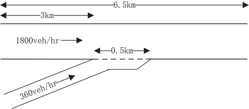
In the highway with an on-ramp, main road flow is usually disturbed by the merging vehicle from ramp flow, which results in frequent acceleration/deceleration of vehicles and has potential increase of emissions and fuel consumption. Moreover, we only focus on the longitudinal movements of vehicles based on car-following models in simulations. Therefore, we select a hypothetical one-lane highway with an on-ramp as the simulation segment, based on the previous studies (Mahmassani 2016; Talebpour and Mahmassani 2016), as shown in Figure 1. All parameters needed for simulations are determined according to the recent studies (Mahmassani 2016; Talebpour and Mahmassani 2016). The main road flow is set as 1800veh/hr, while 360veh/hr is considered as the ramp flow. The initial speed of vehicles upstream is the free-flow speed 33 m/s, the maximum acceleration is set as 4 m/s² and the emergency deceleration is −6 m/s² in the simulations (Ni et al. 2015). Moreover, we mainly focus on the main road flow, while all vehicles can be considered to have same lane-change behaviors when merging from the ramp (Xiao et al. 2018). The Lane Change Model with Relaxation and Synchronization (LMRS) in Schakel, Knoop, and van Arem (2012) is used for merging behaviors.

Figure 1. Geometric characteristics of the simulation segment.

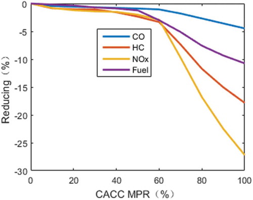
As noted before, simulations were performed by using car-following models described in Section 2, under the mixed traffic flow defined in Section 3.1 for different CACC MPRs. Then, the CO emission, HC emission, NOx emission, and fuel consumption are calculated based on the VT-Micro model (Ahn et al. 2002). Taking into consideration the random vehicle orders in simulations, each simulation was repeated for 10 times to calculate the average values of emissions and fuel consumption. Because the main purpose of this paper is to evaluate emission impacts from qualitative perspective, namely the impact trend with different CACC MPRs in the mixed traffic flow. The emission and fuel consumption results of traffic flow with 0% CACC MPR, i.e., the full MDVs flow, is considered as the benchmark. In addition, the number of vehicles in total depends on the flow rate and the simulation time. Hence, there are always a lot of vehicles in each simulation for every CACC MPR. This satisfies the requirement of microscopic simulations (Qin, He, and Ran 2019).

By comparing this benchmark, percentage changes are obtained for different CACC MPRs, as shown in Figure 2. Note that the CACC desired time gap t_c = 0.6 sec and the ACC desired time gap t_a = 1.1 sec in Figure 2, while parametric sensitivity analysis on t_c and t_a will be performed in the next section. In Figure 2, the increasing stands for that the emissions and fuel consumption are more than the benchmark of the full MDVs flow, while the reducing denotes that the mixed flow with the corresponding CACC MPRs can reduce the emissions and fuel consumption of the full MDVs flow. According to Figure 2, it can be seen that the emissions and fuel consumption will firstly increase and then decrease with the increase of the CACC MPR. Moreover, the worst situation happens when the CACC MPR increases to approximately 30%. Although the emissions and fuel consumption decrease if the CACC MPR exceeds 30%, they cannot be less than those of the full MDVs flow until the CACC MPR reaches about 80%. From 80% to 100% of the CACC MPR, the emissions and fuel consumption can be gradually reduced. The reductions of CO, HC, NOx, and fuel consumption are −4.46%, −17.83%, −27.20%, and −10.74%, respectively, when the full CACC flow is compared with the full MDVs flow.

Figure 2. Percentage changes of emissions and fuel consumption with respect to CACC MPR (t_c = 0.6 sec and t_a = 1.1 sec).

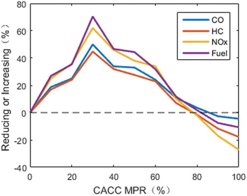
Therefore, the impact trend indicated that the early stage of CACC MPRs will cause more emissions and fuel consumption. Moreover, the emission and fuel consumption situations of the traditional MDVs flow cannot be reduced until the CACC MPR exceeds to a relatively high value (about 80%). We will provide an insight for the results obtained here in the discussion section, from the perspective of traffic flow stability.

Discussions

This section performs parametric sensitivity analysis on CACC desired time gap t_c and ACC desired time gap t_a. Moreover, we also analytically investigate stability of the mixed traffic flow under different CACC MPRs, which provides an insight for the relationship with the emission impacts obtained in this paper.

Parametric sensitivity analysis

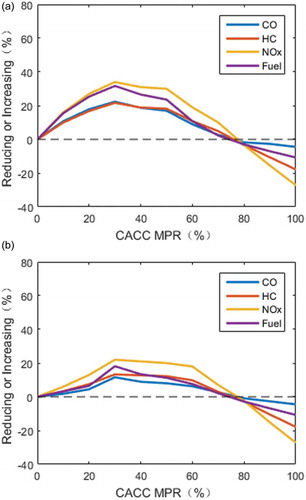
Although the desired time gap t_c and t_a were set as 0.6 sec and 1.1 sec, respectively, in PATH program’s experiments (Milanés and Shladover 2014), their values can be adjusted within a certain range. Based on Shladover, Su, and Lu (2012), t_c changes from 0.6 to 1.1 sec, while t_a has the range of 1.1–2.2 sec. Therefore, we set t_c as 0.6 sec, 0.9 sec, and 1.1 sec and consider t_a to be 1.1 sec, 1.6 sec, and 2.2 sec for the parametric sensitivity analysis. Note that the emission impacts under t_c = 0.6 sec and t_a = 1.1 sec have been evaluated in Figure 2. Then, when parametric sensitivity analysis on t_c is conducted, we keep t_a being 1.1 sec. Also, we maintain t_c = 0.6 s for the parametric sensitivity analysis on t_a. The results of the parametric sensitivity analysis on t_c and t_a are shown in Figures 3 and 4, respectively.

Figure 3. The parametric sensitivity analysis on t_c (t_a = 1.1 sec) of emissions and fuel consumption: (a) t_c = 0.9 sec, (b) t_c = 1.1 sec.

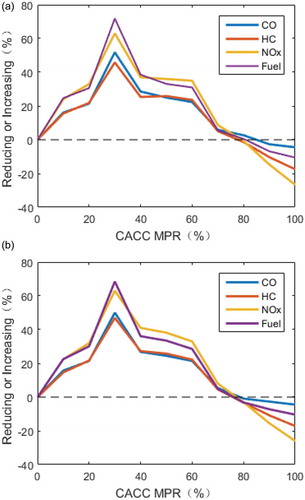
Figure 4. The parametric sensitivity analysis on t_a (t_c = 0.6 sec) of emissions and fuel consumption: (a) t_a = 1.6 sec, (b) t_a = 2.2 sec.

By comparing Figures 2 and 3, it is indicated that different values of t_c almost cannot affect the impact trends of the emissions and fuel consumption with respect to CACC MPRs. Moreover, compared with the full MDVs flow, the reductions of the emissions and fuel consumption are similar for different values of t_c. Therefore, it seems that various t_c has similar influence on the emissions and fuel consumption results, which means t_c = 0.6 sec may be appropriate because smaller value of t_c has more benefits in improving traffic capacity (Shladover, Su, and Lu 2012).

For the case of the parametric sensitivity analysis on t_a, we compare the results in Figures 2 and 4. It can be found that the emissions and fuel consumption also firstly increase and then decrease with the increase of the CACC MPR for different values of t_a. This means the impact trends of the emissions and fuel consumption are still not changed. However, when t_a increases to 2.2 sec, the worse amplitudes are suppressed. This means the worst situation increase CO, HC, NOx, and fuel consumption by 50.00%, 44.76%, 62.00%, and 70.42%, respectively, in Figure 2 with 30% CACC MPR, while the increases are 11.61%, 13.29%, 22.00%, and 18.13%, respectively, in Figure 4(b) compare with the full MDVs. Hence, t_a = 2.2 sec is apt to restrain the deterioration amplitude of the emissions and fuel consumption before the CACC MPR reaches to about 80%, though it cannot change the impact trend.

Traffic flow stability

Stability is one importation property of traffic flow. It is called stable if speed disturbances downstream are smoothed by vehicles upstream, while unstable flow means the disturbances are amplified when spreading through vehicles upstream. Therefore, unstable flow causes large speed disturbances and may result in more emissions and fuel consumption. This section analytically investigates stability of the mixed traffic flow under different CACC MPRs, based on which its relationship with the impact trend of CACC MPRs on the emissions and fuel consumption obtained in this paper will be shown.

Stability of car-following models

The stability of car-following models denotes stability situations of homogenous vehicular flow, which has been widely studied and various methods were proposed to deal with it (Sau et al. 2014; Sun, Zheng, and Sun 2018; Treiber and Kesting 2013; Wilson 2008). Moreover, some studies (Sun, Zheng, and Sun 2018; Treiber and Kesting 2013; Wilson 2008) also presented the generalized instability criterion for the general car-following model of acceleration function with respect to the following vehicle’s speed, spacing, and speed difference to the leading vehicle. The generalized instability criterion of the car-following model is written as follows (Wilson 2008):

(7) $\frac{1}{2}(f_n^v{)}^2-f_n^{\mathrm{\Delta }v}{f}_n^v-f_n^h<0$(7)

where f is the acceleration law of the car-following model, n denotes the vehicle, $f_n^v$, $f_n^{\mathrm{\Delta }v}$, and $f_n^h$ are partial differential of f with respect to speed v, speed difference Δv, and spacing h. The three partial differentials are calculated as follows:

(8) $\left\{\begin{array}{c}{f}_n^v=\frac{\mathrm{\partial }f(v_n,\mathrm{\Delta }{v}_n,h_n)}{\mathrm{\partial }{v}_n}{|}_{(v_e,0,h_e)}\\ f_n^{\mathrm{\Delta }v}=\frac{\mathrm{\partial }f(v_n,\mathrm{\Delta }{v}_n,h_n)}{\mathrm{\partial }\mathrm{\Delta }{v}_n}{|}_{(v_e,0,h_e)}\\ f_n^h=\frac{\mathrm{\partial }f(v_n,\mathrm{\Delta }{v}_n,h_n)}{\mathrm{\partial }{h}_n}{|}_{(v_e,0,h_e)}\end{array}\right.$(8)

where v_e and h_e denote the equilibrium speed and spacing, respectively. It means the traffic flow is unstable if the criterion in Eq. (7)(7) $\frac{1}{2}(f_n^v{)}^2-f_n^{\mathrm{\Delta }v}{f}_n^v-f_n^h<0$(7) is satisfied.

CACC flow

In the case of the CACC car-following model in Eq. (1(1) $\left\{\begin{array}{c}{v}_n(t+\mathrm{\Delta }t)=v_n(t)+k_p{e}_n(t)+k_d{\dot{e}}_n(t)\\ e_n(t)=h_n(t)-t_c{v}_n(t)\end{array}\right.$(1) ), the control step time Δt is very small (0.01 sec). Then, the speed function v_n(t+ Δt) can be transformed into the acceleration form by using the first-order Taylor series expansion:

(9) $v_n(t+\mathrm{\Delta }t)=v_n(t)+\mathrm{\Delta }t{\dot{v}}_n(t)$(9)

Substituting Eq. (9)(9) $v_n(t+\mathrm{\Delta }t)=v_n(t)+\mathrm{\Delta }t{\dot{v}}_n(t)$(9) into Eq. (1)(1) $\left\{\begin{array}{c}{v}_n(t+\mathrm{\Delta }t)=v_n(t)+k_p{e}_n(t)+k_d{\dot{e}}_n(t)\\ e_n(t)=h_n(t)-t_c{v}_n(t)\end{array}\right.$(1) to obtain the CACC car-following model with the acceleration law form:

(10) ${\dot{v}}_n(t)=\frac{k_p\left(h_n(t)-t_c{v}_n(t)\right)+k_d\left(v_{n-1}(t)-v_n(t)\right)}{\mathrm{\Delta }t+k_d{t}_c}$(10)

Substituting Eq. (8)(8) $\left\{\begin{array}{c}{f}_n^v=\frac{\mathrm{\partial }f(v_n,\mathrm{\Delta }{v}_n,h_n)}{\mathrm{\partial }{v}_n}{|}_{(v_e,0,h_e)}\\ f_n^{\mathrm{\Delta }v}=\frac{\mathrm{\partial }f(v_n,\mathrm{\Delta }{v}_n,h_n)}{\mathrm{\partial }\mathrm{\Delta }{v}_n}{|}_{(v_e,0,h_e)}\\ f_n^h=\frac{\mathrm{\partial }f(v_n,\mathrm{\Delta }{v}_n,h_n)}{\mathrm{\partial }{h}_n}{|}_{(v_e,0,h_e)}\end{array}\right.$(8) into Eq. (10)(10) ${\dot{v}}_n(t)=\frac{k_p\left(h_n(t)-t_c{v}_n(t)\right)+k_d\left(v_{n-1}(t)-v_n(t)\right)}{\mathrm{\Delta }t+k_d{t}_c}$(10) to calculate the three partial differentials of the CACC car-following model, which yields

(11) $\left\{\begin{array}{c}{f}_C^v=-\frac{k_p{t}_c}{\mathrm{\Delta }t+k_d{t}_c}\\ f_C^{\mathrm{\Delta }v}=\frac{k_d}{\mathrm{\Delta }t+k_d{t}_c}\\ f_C^h=\frac{k_p}{\mathrm{\Delta }t+k_d{t}_c}\end{array}\right.$(11)

where subscript C denotes the CACC vehicle type.

It can be found that the three partial differentials of CACC model in Eq. (11)(11) $\left\{\begin{array}{c}{f}_C^v=-\frac{k_p{t}_c}{\mathrm{\Delta }t+k_d{t}_c}\\ f_C^{\mathrm{\Delta }v}=\frac{k_d}{\mathrm{\Delta }t+k_d{t}_c}\\ f_C^h=\frac{k_p}{\mathrm{\Delta }t+k_d{t}_c}\end{array}\right.$(11) are only determined by the CACC model parameters and do not depend on the equilibrium speed. By substituting Eq. (11)(11) $\left\{\begin{array}{c}{f}_C^v=-\frac{k_p{t}_c}{\mathrm{\Delta }t+k_d{t}_c}\\ f_C^{\mathrm{\Delta }v}=\frac{k_d}{\mathrm{\Delta }t+k_d{t}_c}\\ f_C^h=\frac{k_p}{\mathrm{\Delta }t+k_d{t}_c}\end{array}\right.$(11) into Eq. (7(7) $\frac{1}{2}(f_n^v{)}^2-f_n^{\mathrm{\Delta }v}{f}_n^v-f_n^h<0$(7) ), we can calculate that the instability criterion in Eq. (7)(7) $\frac{1}{2}(f_n^v{)}^2-f_n^{\mathrm{\Delta }v}{f}_n^v-f_n^h<0$(7) is not satisfied. This means CACC vehicles are always stable for all possible equilibrium speeds.

ACC flow

The ACC car-following model in Eq. (2)(2) ${\dot{v}}_n(t)=k_1\left(h_n(t)-t_a{v}_n(t)\right)+k_2\left(v_{n-1}(t)-v_n(t)\right)$(2) is described as the acceleration function with respect to the following vehicle’s speed, speed difference, and spacing to the leading vehicle. Then, substitute Eq. (8)(8) $\left\{\begin{array}{c}{f}_n^v=\frac{\mathrm{\partial }f(v_n,\mathrm{\Delta }{v}_n,h_n)}{\mathrm{\partial }{v}_n}{|}_{(v_e,0,h_e)}\\ f_n^{\mathrm{\Delta }v}=\frac{\mathrm{\partial }f(v_n,\mathrm{\Delta }{v}_n,h_n)}{\mathrm{\partial }\mathrm{\Delta }{v}_n}{|}_{(v_e,0,h_e)}\\ f_n^h=\frac{\mathrm{\partial }f(v_n,\mathrm{\Delta }{v}_n,h_n)}{\mathrm{\partial }{h}_n}{|}_{(v_e,0,h_e)}\end{array}\right.$(8) into Eq. (2)(2) ${\dot{v}}_n(t)=k_1\left(h_n(t)-t_a{v}_n(t)\right)+k_2\left(v_{n-1}(t)-v_n(t)\right)$(2) to obtain the three partial differentials of the ACC model, as follows:

(12) $\left\{\begin{array}{c}{f}_A^v=-k_1{t}_a\\ f_A^{\mathrm{\Delta }v}=k_2\\ f_A^h=k_1\end{array}\right.$(12)

where subscript A stands for the ACC vehicle type.

Equation (12)(12) $\left\{\begin{array}{c}{f}_A^v=-k_1{t}_a\\ f_A^{\mathrm{\Delta }v}=k_2\\ f_A^h=k_1\end{array}\right.$(12) shows that the ACC model’s partial differentials also do not depend on the equilibrium speed. If Eq. (12)(12) $\left\{\begin{array}{c}{f}_A^v=-k_1{t}_a\\ f_A^{\mathrm{\Delta }v}=k_2\\ f_A^h=k_1\end{array}\right.$(12) is substituted into Eq. (7(7) $\frac{1}{2}(f_n^v{)}^2-f_n^{\mathrm{\Delta }v}{f}_n^v-f_n^h<0$(7) ), it can be calculated that the instability criterion in Eq. (7)(7) $\frac{1}{2}(f_n^v{)}^2-f_n^{\mathrm{\Delta }v}{f}_n^v-f_n^h<0$(7) is satisfied, which means ACC vehicles are unstable for all possible equilibrium speeds. Note that the ACC model in Eq. (2)(2) ${\dot{v}}_n(t)=k_1\left(h_n(t)-t_a{v}_n(t)\right)+k_2\left(v_{n-1}(t)-v_n(t)\right)$(2) was validated by PATH program using real experimental data, which showed the instability of the commercial ACC system when being equipped into the real vehicle at the current control level (Milanés and Shladover 2014).

MDV flow

Based on the MDV’s car-following model in Eq. (3(3) ${\dot{v}}_n(t)=\kappa \left(V(h_n(t))-v_n(t)\right)+\frac{\lambda }{h_n(t)}\left(v_{n-1}(t)-v_n(t)\right)$(3) ), the partial differentials are calculated:

(13) $\left\{\begin{array}{c}{f}_H^v=\kappa \\ f_H^{\mathrm{\Delta }v}=\frac{\lambda }{-(v_0/\alpha )ln(1-v/v_0)+s_0}\\ f_H^h=\kappa \alpha (1-v/v_0)\end{array}\right.$(13)

where H stands for the MDV type.

Equation (13)(13) $\left\{\begin{array}{c}{f}_H^v=\kappa \\ f_H^{\mathrm{\Delta }v}=\frac{\lambda }{-(v_0/\alpha )ln(1-v/v_0)+s_0}\\ f_H^h=\kappa \alpha (1-v/v_0)\end{array}\right.$(13) indicates that the three partial differentials of MDV depend on the equilibrium speed, which means that the stability of MDV is related to the equilibrium speed. We substitute Eq. (13)(13) $\left\{\begin{array}{c}{f}_H^v=\kappa \\ f_H^{\mathrm{\Delta }v}=\frac{\lambda }{-(v_0/\alpha )ln(1-v/v_0)+s_0}\\ f_H^h=\kappa \alpha (1-v/v_0)\end{array}\right.$(13) into Eq. (7)(7) $\frac{1}{2}(f_n^v{)}^2-f_n^{\mathrm{\Delta }v}{f}_n^v-f_n^h<0$(7) to calculate the stability criterion. The calculation result is shown in Figure 5, in which the x-axis is the equilibrium speed and the y-axis is the left side in Eq. 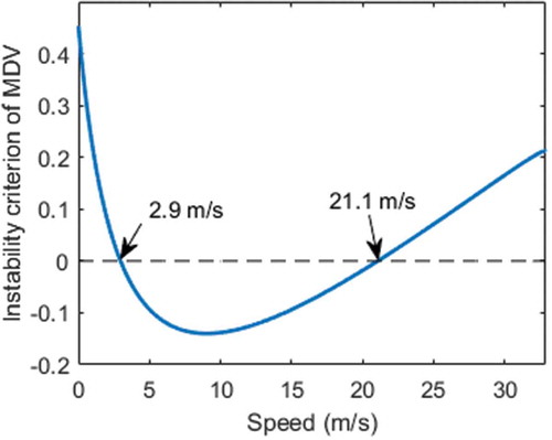(7)(7) $\frac{1}{2}(f_n^v{)}^2-f_n^{\mathrm{\Delta }v}{f}_n^v-f_n^h<0$(7) . According to Figure 5, MDVs are unstable when the equilibrium speed changes from 2.9 m/sec to 21.1 m/sec, while stable for the other speed ranges.

Figure 5. Stability of MDV.

Stability of the mixed flow

Although many studies focused on the stability analysis of the car-following models, only a few works were conducted on analytical investigation of the mixed traffic flow (Mahmassani 2016; Qin and Wang 2018). Among them, Ward (2009) presented a general framework for the stability analysis of the car-truck mixed flow. The analytical framework proposed by Ward (2009) has been extended to the traffic flow mixed with MDVs and CACC/ACC vehicles (Mahmassani 2016; Ngoduy 2013, 2015; Talebpour and Mahmassani 2016; Talebpour, Mahmassani, and Hamdar 2017; Wang et al. 2019a). Here we also employ the guidance of Ward’s framework (Ward 2009) to analytically study the stability of the mixed CACC/ACC flow. Ward (2009) presented the following instability criterion for the mixed traffic flow:

(14) $\sum _n([\frac{1}{2}{(f_n^v)}^2-f_n^{\mathrm{\Delta }v}{f}_n^v-f_n^h]{[\prod _{m\ne n}{f}_m^h]}^2)<0$(14)

where n and m stand for the individual vehicles.

Equation (14)(14) $\sum _n([\frac{1}{2}{(f_n^v)}^2-f_n^{\mathrm{\Delta }v}{f}_n^v-f_n^h]{[\prod _{m\ne n}{f}_m^h]}^2)<0$(14) shows the stability condition does not depend on vehicle orders in the mixed traffic flow, while it is determined by the proportion of each vehicle type (Mahmassani 2016; Ngoduy 2013, 2015; Talebpour and Mahmassani 2016; Talebpour, Mahmassani, and Hamdar 2017; Wang et al. 2019a; Ward 2009). In the mixed traffic flow, described in Section 3.1, focused on by this paper, p_c, p_a, and p_h are used to denote the proportion of CACC vehicles (after the degeneration), ACC vehicle, and MDVs, respectively. Then, the stability framework in Eq. (14)(14) $\sum _n([\frac{1}{2}{(f_n^v)}^2-f_n^{\mathrm{\Delta }v}{f}_n^v-f_n^h]{[\prod _{m\ne n}{f}_m^h]}^2)<0$(14) can be extended to the mixed traffic flow focused on by this paper, as follows:

(15) $p_c\frac{{(f_C^v)}^2-2f_C^{\mathrm{\Delta }v}{f}_C^v-2f_C^h}{2{(f_C^h)}^2}+p_a\frac{{(f_A^v)}^2-2f_A^{\mathrm{\Delta }v}{f}_A^v-2f_A^h}{2{(f_A^h)}^2}+p_h\frac{{(f_M^v)}^2-2f_M^{\mathrm{\Delta }v}{f}_M^v-2f_M^h}{2{(f_M^h)}^2}<0$(15)

Substituting Eq. (6)(6) $\left\{\begin{array}{c}{p}_c=p^2\\ p_a=p(1-p)\\ p_h=1-p\end{array}\right.$(6) into Eq. (15(15) $p_c\frac{{(f_C^v)}^2-2f_C^{\mathrm{\Delta }v}{f}_C^v-2f_C^h}{2{(f_C^h)}^2}+p_a\frac{{(f_A^v)}^2-2f_A^{\mathrm{\Delta }v}{f}_A^v-2f_A^h}{2{(f_A^h)}^2}+p_h\frac{{(f_M^v)}^2-2f_M^{\mathrm{\Delta }v}{f}_M^v-2f_M^h}{2{(f_M^h)}^2}<0$(15) ), we have

(16) $\begin{array}{rl}& \left(\frac{{(f_C^v)}^2-2f_C^{\mathrm{\Delta }v}{f}_C^v-2f_C^h}{2{(f_C^h)}^2}-\frac{{(f_A^v)}^2-2f_A^{\mathrm{\Delta }v}{f}_A^v-2f_A^h}{2{(f_A^h)}^2}\right)p^2-\\ & \left(\frac{{(f_M^v)}^2-2f_M^{\mathrm{\Delta }v}{f}_M^v-2f_M^h}{2{(f_M^h)}^2}-\frac{{(f_A^v)}^2-2f_A^{\mathrm{\Delta }v}{f}_A^v-2f_A^h}{2{(f_A^h)}^2}\right)p+\\ & \frac{{(f_M^v)}^2-2f_M^{\mathrm{\Delta }v}{f}_M^v-2f_M^h}{2{(f_M^h)}^2}<0\end{array}$(16)

Equation (16)(16) $\begin{array}{rl}& \left(\frac{{(f_C^v)}^2-2f_C^{\mathrm{\Delta }v}{f}_C^v-2f_C^h}{2{(f_C^h)}^2}-\frac{{(f_A^v)}^2-2f_A^{\mathrm{\Delta }v}{f}_A^v-2f_A^h}{2{(f_A^h)}^2}\right)p^2-\\ & \left(\frac{{(f_M^v)}^2-2f_M^{\mathrm{\Delta }v}{f}_M^v-2f_M^h}{2{(f_M^h)}^2}-\frac{{(f_A^v)}^2-2f_A^{\mathrm{\Delta }v}{f}_A^v-2f_A^h}{2{(f_A^h)}^2}\right)p+\\ & \frac{{(f_M^v)}^2-2f_M^{\mathrm{\Delta }v}{f}_M^v-2f_M^h}{2{(f_M^h)}^2}<0\end{array}$(16) transforms the stability condition of the mixed flow into the parabolic function of CACC MPR p (the left side of Eq. (16)(16) $\begin{array}{rl}& \left(\frac{{(f_C^v)}^2-2f_C^{\mathrm{\Delta }v}{f}_C^v-2f_C^h}{2{(f_C^h)}^2}-\frac{{(f_A^v)}^2-2f_A^{\mathrm{\Delta }v}{f}_A^v-2f_A^h}{2{(f_A^h)}^2}\right)p^2-\\ & \left(\frac{{(f_M^v)}^2-2f_M^{\mathrm{\Delta }v}{f}_M^v-2f_M^h}{2{(f_M^h)}^2}-\frac{{(f_A^v)}^2-2f_A^{\mathrm{\Delta }v}{f}_A^v-2f_A^h}{2{(f_A^h)}^2}\right)p+\\ & \frac{{(f_M^v)}^2-2f_M^{\mathrm{\Delta }v}{f}_M^v-2f_M^h}{2{(f_M^h)}^2}<0\end{array}$(16) ). This means the mixed traffic flow is unstable when the parabolic function is below the horizontal axis. Based on Eqs. (11(11) $\left\{\begin{array}{c}{f}_C^v=-\frac{k_p{t}_c}{\mathrm{\Delta }t+k_d{t}_c}\\ f_C^{\mathrm{\Delta }v}=\frac{k_d}{\mathrm{\Delta }t+k_d{t}_c}\\ f_C^h=\frac{k_p}{\mathrm{\Delta }t+k_d{t}_c}\end{array}\right.$(11) )–(13(13) $\left\{\begin{array}{c}{f}_H^v=\kappa \\ f_H^{\mathrm{\Delta }v}=\frac{\lambda }{-(v_0/\alpha )ln(1-v/v_0)+s_0}\\ f_H^h=\kappa \alpha (1-v/v_0)\end{array}\right.$(13) ), it can be found that not only p but also the equilibrium speed determines the values of the parabolic function. Therefore, the stability conditions of the mixed traffic flow are related to CACC MPR p and equilibrium speeds. Taking into consideration each equilibrium speed, we can calculate the values of the parabolic function under each value of p, which means the stability chart with respect to CACC MPR p and the equilibrium speed can be obtained. Moreover, we can calculate critical values of p that make the lowest values of the parabolic function under the corresponding speeds, based on the properties of the parabola. Besides, when p is equal to be 0, the instability criterion in Eq. (16)(16) $\begin{array}{rl}& \left(\frac{{(f_C^v)}^2-2f_C^{\mathrm{\Delta }v}{f}_C^v-2f_C^h}{2{(f_C^h)}^2}-\frac{{(f_A^v)}^2-2f_A^{\mathrm{\Delta }v}{f}_A^v-2f_A^h}{2{(f_A^h)}^2}\right)p^2-\\ & \left(\frac{{(f_M^v)}^2-2f_M^{\mathrm{\Delta }v}{f}_M^v-2f_M^h}{2{(f_M^h)}^2}-\frac{{(f_A^v)}^2-2f_A^{\mathrm{\Delta }v}{f}_A^v-2f_A^h}{2{(f_A^h)}^2}\right)p+\\ & \frac{{(f_M^v)}^2-2f_M^{\mathrm{\Delta }v}{f}_M^v-2f_M^h}{2{(f_M^h)}^2}<0\end{array}$(16) becomes that for homogenous MDVs, while that for homogenous CACC flow if p increases to 1. Therefore, we can also calculate the critical values of p that make the parabolic has the same values with those when p = 0, under the corresponding speeds.

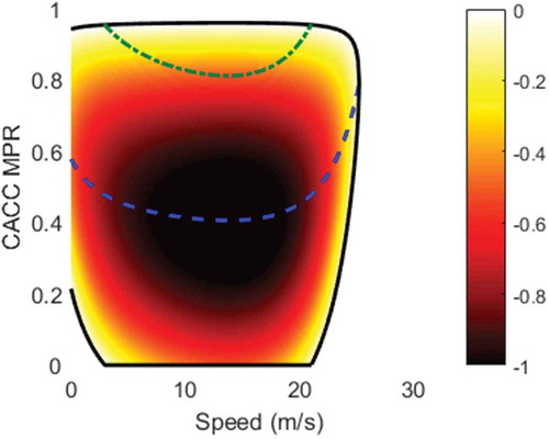
Following the above instability criterion and the general analytical framework (Wang et al. 2019a), we calculate the stability chart for the mixed traffic flow, as shown in Figure 6, in which CACC desired time gap t_c = 0.6 sec and ACC desired time gap t_a = 1.1 sec. In Figure 6, the color values below 0 denote instability for the corresponding CACC MPR p and equilibrium speeds. Therefore, the region within the range of the black curve stands for instability, while the outside region stands for stable flow. The blue curve below illustrates the critical values of p that make the lowest values of the parabolic function under the corresponding speeds, which indicates the worst instability situation. Moreover, the green curve above stands for the critical values of p that make the parabolic has the same values with those when p = 0, which indicates the same instability condition with the homogenous MDVs under the corresponding speeds. According to Figure 6, it can be found that the instability of homogenous MDVs will be worsened with the increase of CACC MPR p, which indicates the worst situation happens if p increases to about 0.4. After that, the instability of homogenous MDVs will be gradually improved and will be recovered when p increases to about 0.8 to 0.9 under some speeds. But the mixed traffic flow is still unstable until p exceeds 0.9. By comparing Figures 2 and 6, we found that there is a qualitative relationship between impact trend of emissions and fuel consumption and stability of the mixed traffic flow, with respect to CACC MPRs. It indicates that the stability situations qualitatively influence the impact trend of CACC MPRs on the emissions and fuel consumption. Meanwhile, we also mention that the corresponding critical values of CACC MPRs are close but not exactly the same between Figures 2 and 6, because it is hard to find a quantitative relationship.

Figure 6. Stability chart of the mixed traffic flow (t_c = 0.6 sec and t_a = 1.1 sec).

In Section 4.1, parametric sensitivity analysis on t_c and t_a are conducted for emissions and fuel consumption evaluation. Therefore, these two types of parametric sensitivity analyses are also performed for the stability chart of the mixed traffic flow, as shown in Figures 7 and 8. The parametric sensitivity analysis on t_c is conducted in Figure 7, while the parametric sensitivity analysis on t_a is conducted in Figure 8. By comparing Figures 6 and 7, we found that different values of t_c almost have no different impacts on stability of the mixed flow, which may be a reason for the results obtained in Figures 2 and 3. By comparing Figures 6 and 8, we found that larger value of t_a is apt to restrain the deterioration of stability of the mixed traffic flow, while it still cannot avoid the occurrence of the stability deterioration. Therefore, parametric sensitivity analysis on t_c and t_a of stability of the mixed traffic flow also shows the qualitative relationship with the impact trend of CACC MPRs on the emissions and fuel consumption.

Figure 7. Stability chart of the mixed flow with parametric sensitivity analysis on t_c (t_a = 1.1 sec): (a) t_c = 0.9 sec, (b) t_c = 1.1 sec.

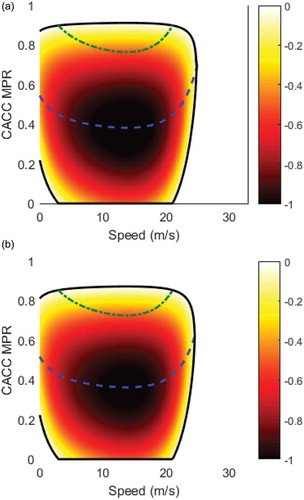
Figure 8. Stability chart of the mixed flow with parametric sensitivity analysis on t_a (t_c = 0.6 sec): (a) t_a = 1.6 sec, (b) t_a = 2.2 sec.

V2 V communication environment

The CACC and ACC models used in this paper are validated by PATH program using real experimental date (Milanés and Shladover 2014), which shows the unstable ACC vehicular flow and the stable CACC vehicular flow. Therefore, unstable ACC vehicles have the negative impacts on stability of the mixed traffic flow, thereby causing more emissions and fuel consumption than the homogenous MDV flow. To confirm this, we assume that all MDVs are equipped with V2 V communication devices. It only requires that MDVs share their moving information to CACC vehicles via V2 V communication devices, which has been conducted by real experiments and would be achieved in future connected vehicular network (Ge et al. 2018). Then, in the V2 V communication environment, CACC vehicles will not degenerate to ACC vehicles and there are no ACC vehicles in the mixed traffic flow. The CACC time gap t_c is desired to be 0.6 s for improving traffic capacity. We still use p denotes the CACC MPR. Then, proportion of CACC vehicles and MDVs are p and 1-p, respectively, in the V2 V communication environment. Hence, the stability framework in Eq. (14)(14) $\sum _n([\frac{1}{2}{(f_n^v)}^2-f_n^{\mathrm{\Delta }v}{f}_n^v-f_n^h]{[\prod _{m\ne n}{f}_m^h]}^2)<0$(14) is extended as follows:

(17) $p\frac{{(f_C^v)}^2-2f_C^{\mathrm{\Delta }v}{f}_C^v-2f_C^h}{2{(f_C^h)}^2}+(1-p)\frac{{(f_M^v)}^2-2f_M^{\mathrm{\Delta }v}{f}_M^v-2f_M^h}{2{(f_M^h)}^2}<0$(17)

Substituting Eqs. (11(11) $\left\{\begin{array}{c}{f}_C^v=-\frac{k_p{t}_c}{\mathrm{\Delta }t+k_d{t}_c}\\ f_C^{\mathrm{\Delta }v}=\frac{k_d}{\mathrm{\Delta }t+k_d{t}_c}\\ f_C^h=\frac{k_p}{\mathrm{\Delta }t+k_d{t}_c}\end{array}\right.$(11) )–(13(13) $\left\{\begin{array}{c}{f}_H^v=\kappa \\ f_H^{\mathrm{\Delta }v}=\frac{\lambda }{-(v_0/\alpha )ln(1-v/v_0)+s_0}\\ f_H^h=\kappa \alpha (1-v/v_0)\end{array}\right.$(13) ) into Eq. 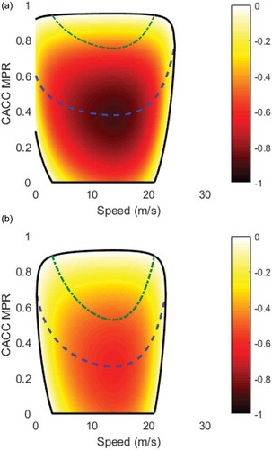(17(17) $p\frac{{(f_C^v)}^2-2f_C^{\mathrm{\Delta }v}{f}_C^v-2f_C^h}{2{(f_C^h)}^2}+(1-p)\frac{{(f_M^v)}^2-2f_M^{\mathrm{\Delta }v}{f}_M^v-2f_M^h}{2{(f_M^h)}^2}<0$(17) ), we can calculate the stability chart of the mixed CACC flow with respect to CACC MPR p and equilibrium speeds, as shown in Figure 9. In Figure 9, the region under the black curve denotes instability, while the outside region stands for the stable flow. It can be seen that the instability of homogenous MDV flow is gradually improved toward the stable situation. In addition, we also conducted simulations for evaluation of emissions and fuel consumption in the V2 V communication environment. The simulation results are shown in Figure 10. According to Figure 10, the emissions and fuel consumption of the homogenous MDV flow are gradually reduced with the increase of the CACC MPR in the V2 V communication environment. The full CACC flow can reduce CO, HC, NOx, and fuel consumption by about 4.46%, 17.83%, 27.20%, and 10.74%, respectively, compared with the full MDV flow, though the reduction is small when the CACC MPR is no more than approximately 60%. Figures 9 and 10 also show that the stability situations qualitatively influence the impact trend of CACC MPRs on the emissions and fuel consumption. In addition, based on the comparison among Figures 2, 6, 9, and 10, V2 V equipments on MDVs are not only encouraging but also essential to avoid the deterioration of stability and emissions in the mixed traffic flow.

Figure 9. Stability chart of mixed CACC flow with V2 V communication environment.

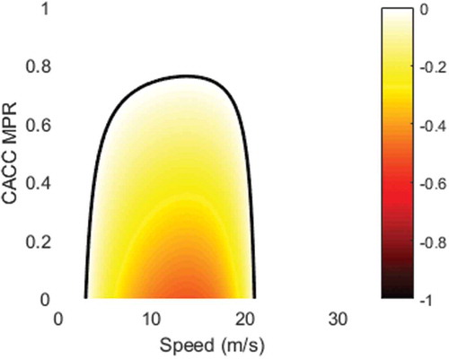
Figure 10. Trend impact of CACC MPRs on emissions and fuel consumption with V2 V communication environment.

We should mention that the results are obtained based on PATH program’s CACC and ACC models, which can represent one class of CACC and ACC models, but not all the models. However, CACC vehicles will always degenerate to ACC vehicles when V2 V communication is not available. Moreover, as long as ACC vehicles are unstable, they will have negative impacts on stability and emissions. Therefore, the qualitative relationship between stability and emissions trend obtained by this paper is always useful for analyzing impacts of CACC/ACC models on emissions. Additionally, the obtained qualitative relationship in this paper also points out the essential of the V2 V equipments on MDVs as long as ACC vehicles are unstable.

Conclusion

Previous studies investigated reductions of some intelligent vehicular systems on emissions. However, some intelligent vehicular systems, such as CACC systems, require V2 V communication environment. In the absent of V2 V communication, CACC system will inherently degenerate to the ACC function as an alternative fallback option. If the ACC function is unstable, it may have negative impacts on emissions. Moreover, by using experimental data, PATH program validated that ACC system is apt to be unstable when being equipped with real vehicles at the present control level (Milanés and Shladover 2014). Therefore, it is important to evaluate the impacts of partial degenerations from stable CACC vehicles to unstable ACC vehicles on emissions in the mixed CACC-MDVs traffic flow. This evaluation was usually lost in previous studies, but focused on by this paper. In addition, traffic flow stability reveals the dynamics of disturbances spreading through vehicles, which may influence the emission impacts in the traffic flow. However, little research was conducted on the relationship of emission evaluations and stability of the mixed CACC-MDVs traffic flow. This paper presents an effort to deal with it and then provide an insight for reducing the emissions.

It is found that the partial degenerations from stable CACC vehicles to unstable ACC vehicles in the mixed CACC-MDVs traffic flow has negative impacts on emissions and fuel consumption. Compared with the full MDVs traffic flow, the CO emission, HC emission, NOx emission, and fuel consumption firstly increase and then decrease with the increase of the CACC MPR. Specifically, the mixed traffic flow produces more emissions and fuel consumption than the full MDVs flow when the CACC MPR is no more than approximately 80%. Parametric sensitivity analysis on CACC and ACC desired time gap also shows this impact trend of the emissions and fuel consumption. Based on the stability analysis of the mixed traffic flow, it indicates that stability situations qualitatively influence the impact trend of CACC MPRs on the emissions and fuel consumption. In addition, in the V2 V communication environment, the stable CACC vehicles no longer degenerate to the unstable ACC vehicles in the mixed traffic flow. Then, the emissions and fuel consumption of the full MDVs flow can be gradually reduced with the increase of the CACC MPR. Compared with the full MDVs flow, the full CACC traffic flow can reduce CO, HC, NOx, and fuel consumption by about 4.46%, 17.83%, 27.20%, and 10.74%, respectively.

The results in this paper are obtained based on PATH program’s CACC and ACC models validated by real experiments, which relatively guarantees the reliable results. We should also mention that the CACC system and ACC system in PATH program’s real experiments are specific systems, which cannot represent all types of CACC systems and ACC systems. However, CACC vehicles will always degenerate to ACC vehicles when V2 V communication is not available. As long as ACC vehicles are unstable, they will have negative impacts on emissions and fuel consumption. Therefore, the qualitative relationship between stability and emissions trend obtained by this paper is always useful for analyzing impacts of CACC/ACC models on emissions. Moreover, it can be obtained that V2 V communication equipments on MDVs are not only encouraging but also essential to avoid the deterioration of emissions and fuel consumption in the mixed traffic flow, as long as ACC vehicles are unstable.

There are two ways to avoid deterioration of emissions and fuel consumption of the mixed traffic flow, compared with the full MDVs flow: (1) develop stable ACC systems; and (2) implement V2 V communication equipments on MDVs. PATH program pointed out that although the commercial ACC system was designed by seriously taking stability into consideration, it was actually unstable when being implemented into real vehicles at the current control level (Milanés and Shladover 2014). Therefore, this paper assumes that ACC systems are apt to be unstable. In the case of the second way, it will last a long period of time to completely accomplish implementations of V2 V devices on all MDVs. Before the complete implementations, there are still unstable ACC vehicles degenerated from CACC vehicles in the mixed traffic flow. During this period of time, appropriate emission control strategies should be studied to restrain the negative influence of unstable ACC vehicles on emissions and fuel consumption. This will be left in the next research step.

Disclosure statement

No potential conflict of interest was reported by the authors.

Additional information

Funding

This work is supported by the National Key R&D Program in China (2018YFB1601000), the Science and Technology Research Program of Chongqing Municipal Education Commission (KJQN201900730), the Chongqing Key Project of Technological Innovation and Application Demonstration (cstc2018jscx-mszdX0112), and the Research Foundation for Talented Scholars of Chongqing Jiaotong University (19JDKJC-C003).

Notes on contributors

Yanyan Qin

Yanyan Qin is a assistant professor at School of Traffic and Transportation, Chongqing Jiaotong University, Chongqing, China.

Xinghua Hu

Xinghua Hu is a professors at School of Traffic and Transportation, Chongqing Jiaotong University, Chongqing, China.

Zhaoyi He

Zhaoyi He is a professors at School of Traffic and Transportation, Chongqing Jiaotong University, Chongqing, China.

Shuqing Li

Shuqing Li is a professors at School of Traffic and Transportation, Chongqing Jiaotong University, Chongqing, China.

References

- Ahn, K., H. Rakha, A. Trani, and M. Van Aerde. 2002. Estimating vehicle fuel consumption and emissions based on instantaneous speed and acceleration levels. J. Transp. Eng. 128 (2):182–90. doi:10.1061/(ASCE)0733-947X(2002)128:2(182).
- Bando, M., K. Hasebe, A. Nakayama, A. Shibata, and Y. Sugiyama. 1995. Dynamical model of traffic congestion and numerical simulation. Phys. Rev. E 51 (2):1035–42. doi:10.1103/PhysRevE.51.1035.
- Barth, M., F. An, T. Younglove, C. Levine, G. Scora, M. Ross, and T. Wenzel. 2000. Development of a comprehensive modal emissions model. National Cooperative Highway Research Program, Transportation Research Board of the National Academies.
- Barth, M., and K. Boriboonsomsin. 2009. Energy and emissions impacts of a freeway-based dynamic eco-driving system. Transp. Res. Part D 14 (6):400–10. doi:10.1016/j.trd.2009.01.004.
- Chen, D., J. Laval, Z. Zheng, and S. Ahn. 2012. A behavioral car-following model that captures traffic oscillations. Transp. Res. Part B 46 (6):744–61. doi:10.1016/j.trb.2012.01.009.
- Fagnant, D. J., and K. M. Kockelman. 2014. The travel and environmental implications of shared autonomous vehicles, using agent-based model scenarios. Transp. Res. Part C 40:1–13. doi:10.1016/j.trc.2013.12.001.
- Ge, J. I., S. S. Avedisov, C. R. He, W. B. Qin, M. Sadeghpour, and G. Orosz. 2018. Experimental validation of connected automated vehicle design among human-driven vehicles. Transp. Res. Part C 91:335–52. doi:10.1016/j.trc.2018.04.005.
- Gramsch, E., V. Papapostolou, F. Reyes, Y. Vásquez, M. Castillo, P. Oyola, … J. Lawrence. 2018. Variability in the primary emissions and secondary gas and particle formation from vehicles using bioethanol mixtures. J. Air Waste Manage. Assoc. 68 (4):329–46.
- Hausberger, S., J. Rodler, P. Sturm, and M. Rexeis. 2003. Emission factors for heavy-duty vehicles and validation by tunnel measurements. Atmos. Environ. 37 (37):5237–45. doi:10.1016/j.atmosenv.2003.05.002.
- Hoogendoorn, R., B. van Arerm, and S. Hoogendoom. 2014. Automated driving, traffic flow efficiency, and human factors: Literature review. Transp. Res. Rec. 2422 (1):113–20. doi:10.3141/2422-13.
- Ioannou, P. A., and M. Stefanovic. 2005. Evaluation of ACC vehicles in mixed traffic: Lane change effects and sensitivity analysis. IEEE Trans. Intell. Transp. Syst. 6 (1):79–89. doi:10.1109/TITS.2005.844226.
- Jeong, E., C. Oh, and G. Lee. 2015. Emission evaluation of inter-vehicle safety warning information systems. Transp. Res. Part D 41:106–17. doi:10.1016/j.trd.2015.09.018.
- Jiang, R., Q. Wu, and Z. Zhu. 2001. Full velocity difference model for a car-following theory. Phys. Rev. E 64 (1):017101. doi:10.1103/PhysRevE.64.017101.
- Koupal, J., H. Michaels, M. Cumberworth, C. Bailey, and D. Brzezinski, (2002). Epa’s plan for moves: A comprehensive mobile source emissions model. In: Proceedings of the 12th CRC On-Road Vehicle Emissions Workshop, San Diego, CA.
- Kudoh, Y., H. Ishitani, R. Matsuhashi, Y. Yoshida, K. Morita, S. Katsuki, and O. Kobayashi. 2001. Environmental evaluation of introducing electric vehicles using a dynamic traffic-flow model. Appl. Energy 69 (2):145–59. doi:10.1016/S0306-2619(01)00005-8.
- Lee, J., and B. Park. 2012. Development and evaluation of a cooperative vehicle intersection control algorithm under the connected vehicles environment. IEEE Trans. Intell. Transp. Syst. 13 (1):81–90. doi:10.1109/TITS.2011.2178836.
- Li, X., J. Cui, S. An, and M. Parsafard. 2014. Stop-and-go traffic analysis: Theoretical properties, environmental impacts and oscillation mitigation. Transp. Res. Part B 70:319–39. doi:10.1016/j.trb.2014.09.014.
- Liang, Y., Q. Zha, W. Wang, L. Cui, K. H. Lui, K. F. Ho, … T. Wang. 2017. Revisiting nitrous acid (HONO) emission from on-road vehicles: A tunnel study with a mixed fleet. J. Air Waste Manage. Assoc. 67 (7):797–805. doi:10.1080/10962247.2017.1293573.
- Liu, H., S. E. Shladover, X. Y. Lu, and X. Kan. 2020. Freeway vehicle fuel efficiency improvement via cooperative adaptive cruise control. J. Intell. Transp. Syst. 1–13. doi:10.1080/15472450.2020.1720673.
- Ma, J., X. Li, F. Zhou, J. Hu, and B. B. Park. 2017. Parsimonious shooting heuristic for trajectory design of connected automated traffic part II: Computational issues and optimization. Transp. Res. Part B 95:421–41. doi:10.1016/j.trb.2016.06.010.
- Mahmassani, H. S. 2016. 50th anniversary invited article—autonomous vehicles and connected vehicle systems: Flow and operations considerations. Transp. Sci. 50 (4):1140–62. doi:10.1287/trsc.2016.0712.
- Milakis, D., B. Van Arem, and B. Van Wee. 2017. Policy and society related implications of automated driving: A review of literature and directions for future research. J. Intell. Transp. Syst. 21 (4):324–48. doi:10.1080/15472450.2017.1291351.
- Milanés, V., and S. E. Shladover. 2014. Modeling cooperative and autonomous adaptive cruise control dynamic responses using experimental data. Transp. Res. Part C 48:285–300. doi:10.1016/j.trc.2014.09.001.
- Milanés, V., S. E. Shladover, J. Spring, C. Nowakowski, H. Kawazoe, and M. Nakamura. 2014. Cooperative adaptive cruise control in real traffic situations. IEEE Trans. Intell. Transp. Syst. 15 (1):296–305. doi:10.1109/TITS.2013.2278494.
- Newell, G. F. 1961. Nonlinear effects in the dynamics of car following. Oper. Res. 9 (2):209–29. doi:10.1287/opre.9.2.209.
- Ngoduy, D. 2013. Analytical studies on the instabilities of heterogeneous intelligent traffic flow. Commun. Nonlinear Sci. Numer. Simul. 18 (10):2699–706. doi:10.1016/j.cnsns.2013.02.018.
- Ngoduy, D. 2015. Effect of the car-following combinations on the instability of heterogeneous traffic flow. Transportmetrica B Transp. Dyn. 3 (1):44–58.
- Ni, D., J. D. Leonard, C. Jia, and J. Wang. 2015. Vehicle longitudinal control and traffic stream modeling. Transp. Sci. 50 (3):1016–31. doi:10.1287/trsc.2015.0614.
- Norlund, E. K., and I. Gribkovskaia. 2017. Environmental performance of speed optimization strategies in offshore supply vessel planning under weather uncertainty. Transp. Res. Part D 57:10–22. doi:10.1016/j.trd.2017.08.002.
- Nowakowski, C., D. Thompson, S. E. Shladover, A. Kailas, and X. Y. Lu (2016a). Operational concepts for truck cooperative adaptive cruise control (CACC) maneuvers. In Transportation Research Board 95th Annual Meeting (No. 16–4462), Washington DC.
- Nowakowski, C., D. Thompson, S. E. Shladover, A. Kailas, and X. Y. Lu. 2016b. Operational concepts for truck maneuvers with cooperative adaptive cruise control. Transp. Res. Rec. 2559 (1):57–64. doi:10.3141/2559-07.
- Papageorgiou, M., E. Kosmatopoulos, and I. Papamichail. 2008. Effects of variable speed limits on motorway traffic flow. Transp. Res. Rec. (2047):37–48. doi:10.3141/2047-05.
- Ploeg, J., E. Semsar-Kazerooni, G. Lijster, N. van de Wouw, and H. Nijmeijer. 2015. Graceful degradation of cooperative adaptive cruise control. IEEE Trans. Intell. Transp. Syst. 16 (1):488–97. doi:10.1109/TITS.2014.2349498.
- Pueboobpaphan, R., and B. Van Arem. 2010. Driver and vehicle characteristics and platoon and traffic flow stability: Understanding the relationship for design and assessment of cooperative adaptive cruise control. Transp. Res. Rec. (2189):89–97. doi:10.3141/2189-10.
- Qin, Y., Z. He, and B. Ran. 2019. Rear-end crash risk of CACC-manual driven mixed flow considering the degeneration of CACC systems. IEEE Access 7 (1):140421–29. doi:10.1109/ACCESS.2019.2941496.
- Qin, Y., and H. Wang. 2018. Analytical framework of string stability of connected and autonomous platoons with electronic throttle angle feedback. Transportmetrica A Transp. Sci. 1–22. doi:10.1080/23249935.2018.1518964.
- Qin, Y., H. Wang, and B. Ran. 2018. Control design for stable connected cruise control systems to enhance safety and traffic efficiency. IET Intel. Transport Syst. 12 (8):921–30. doi:10.1049/iet-its.2018.5271.
- Ramezani, H., X. Y. Lu, and S. E. Shladover (2019). Calibration of motor vehicle emission simulator (MOVES) using real heavy-duty truck data. In Transportation Research Board 98th Annual Meeting (No. 19-05836), Washington DC.
- Sau, J., J. Monteil, R. Billot, and N. E. El Faouzi. 2014. The root locus method: Application to linear stability analysis and design of cooperative car-following models. Transportmetrica B Transp. Dyn. 2 (1):60–82.
- Schakel, W. J., V. L. Knoop, and B. van Arem. 2012. Integrated lane change model with relaxation and synchronization. Transp. Res. Rec. 2316 (1):47–57. doi:10.3141/2316-06.
- Shladover, S., D. Su, and X. Y. Lu. 2012. Impacts of cooperative adaptive cruise control on freeway traffic flow. Transp. Res. Rec. (2324):63–70. doi:10.3141/2324-08.
- Shladover, S. E., and C. Nowakowski. 2019. Regulatory challenges for road vehicle automation: Lessons from the california experience. Transp. Res. Part A 122:125–33.
- Sun, J., Z. Zheng, and J. Sun. 2018. Stability analysis methods and their applicability to car-following models in conventional and connected environments. Transp. Res. Part B 109:212–37. doi:10.1016/j.trb.2018.01.013.
- Sun, Z., P. Hao, X. J. Ban, and D. Yang. 2015. Trajectory-based vehicle energy/emissions estimation for signalized arterials using mobile sensing data. Transp. Res. Part D 34:27–40. doi:10.1016/j.trd.2014.10.005.
- Taiebat, M., S. Stolper, and M. Xu. 2019. Forecasting the impact of connected and automated vehicles on energy use: A microeconomic study of induced travel and energy rebound. Appl. Energy 247:297–308. doi:10.1016/j.apenergy.2019.03.174.
- Talebpour, A., and H. S. Mahmassani. 2016. Influence of connected and autonomous vehicles on traffic flow stability and throughput. Transp. Res. Part C 71:143–63. doi:10.1016/j.trc.2016.07.007.
- Talebpour, A., H. S. Mahmassani, and S. H. Hamdar. 2017. Effect of information availability on stability of traffic flow: Percolation theory approach. Transp. Res. Procedia 23:81–100. doi:10.1016/j.trpro.2017.05.006.
- Tang, T. Q., H. J. Huang, and H. Y. Shang. 2015. Influences of the driver’s bounded rationality on micro driving behavior, fuel consumption and emissions. Transp. Res. Part D 41:423–32. doi:10.1016/j.trd.2015.10.016.
- Treiber, M., A. Hennecke, and D. Helbing. 2000. Congested traffic states in empirical observations and microscopic simulations. Phys. Rev. E 62 (2):1805–24. doi:10.1103/PhysRevE.62.1805.
- Treiber, M., and A. Kesting. 2013. Traffic flow dynamics: Data, models and simulation. Berlin, Heidelberg: Springer Berlin Heidelberg.
- Wang, H., Y. Qin, W. Wang, and J. Chen. 2019a. Stability of CACC-manual heterogeneous vehicular flow with partial CACC performance degrading. Transportmetrica B Transp. Dyn. 7 (1):788–813.
- Wang, H., W. Wang, J. Chen, C. C. Xu, and Y. Li. 2019b. Can we trust the speed-spacing relationship estimated by car-following model from non-stationary trajectory data? Transportmetrica A Transp. Sci. 15 (2):263–84. doi:10.1080/23249935.2018.1466211.
- Wang, M., W. Daamen, S. P. Hoogendoorn, and B. van Arem. 2014a. Rolling horizon control framework for driver assistance systems. Part I: Mathematical formulation and non-cooperative systems. Transp. Res. Part C 40:271–89. doi:10.1016/j.trc.2013.11.023.
- Wang, M., W. Daamen, S. P. Hoogendoorn, and B. van Arem. 2014b. Rolling horizon control framework for driver assistance systems. Part II: Cooperative sensing and cooperative control. Transp. Res. Part C 40:290–311. doi:10.1016/j.trc.2013.11.024.
- Ward, J. A. (2009). Heterogeneity, lane-changing and instability in traffic: A mathematical approach (Doctoral dissertation, University of Bristol).
- Wilson, R. E. 2008. Mechanisms for spatio-temporal pattern formation in highway traffic models. Phil. Trans. Royal Soc. London A Math. Phys. Eng. Sci. 366 (1872):2017–32. doi:10.1098/rsta.2008.0018.
- Wu, C., G. Zhao, and B. Ou. 2011. A fuel economy optimization system with applications in vehicles with human drivers and autonomous vehicles. Transp. Res. Part D 16 (7):515–24. doi:10.1016/j.trd.2011.06.002.
- Xiao, L., M. Wang, W. Schakel, and B. van Arem. 2018. Unravelling effects of cooperative adaptive cruise control deactivation on traffic flow characteristics at merging bottlenecks. Transp. Res. Part C 96:380–97. doi:10.1016/j.trc.2018.10.008.
- Yang, H., L. Andres, Z. Sun, Q. Gan, and W. L. Jin. 2018. Field tests of a dynamic green driving strategy based on inter-vehicle communication. Transp. Res. Part D 59: doi: 10.1016/j.trd.2018.01.009.
- Yang, H., and W. L. Jin. 2014. A control theoretic formulation of green driving strategies based on inter-vehicle communications. Transp. Res. Part C 41:48–60. doi:10.1016/j.trc.2014.01.016.
- Yao, H., J. Cui, X. Li, Y. Wang, and S. An. 2018. A trajectory smoothing method at signalized intersection based on individualized variable speed limits with location optimization. Transp. Res. Part D 62:456–73. doi:10.1016/j.trd.2018.03.010.
- Yu, H., Z. Fang, F. Lu, A. T. Murray, H. Zhang, P. Peng, … J. Chen. 2019. Impact of oil price fluctuations on tanker maritime network structure and traffic flow changes. Appl. Energy 237:390–403. doi:10.1016/j.apenergy.2019.01.011.
- Zavala, M., J. I. Huertas, D. Prato, A. Jazcilevich, A. Aguilar, M. Balam, … L. T. Molina. 2017. Real-world emissions of in-use off-road vehicles in Mexico. J. Air Waste Manage. Assoc. 67 (9):958–72. doi:10.1080/10962247.2017.1310677.
- Zhou, F., X. Li, and J. Ma. 2017. Parsimonious shooting heuristic for trajectory design of connected automated traffic part I: Theoretical analysis with generalized time geography. Transp. Res. Part B 95:394–420. doi:10.1016/j.trb.2016.05.007.