Trends in particle matter and its elemental composition in Santiago de Chile, 2011 – 2018

ABSTRACT

Daily fine (PM_2.5) and coarse (PM_10-2.5) particle matter (PM) samples collected at Parque O’Higgins station in downtown Santiago de Chile have been studied to find the trends in concentration from 1998 to 2018. Elemental concentration was obtained using X-ray fluorescence (XRF). Regression models from previous studies indicate that the PM_2.5 and PM_10-2.5 fractions have had a continuous decrease since 1988 mostly due to several policy control measures carried out over several decades. PM_2.5 has decreased from 68.3 in 1988 to 27.6 μg/m³ in 2018 (60.4%). However, if only the last 8 years are considered (2011–2018), a leveling off can be observed in PM_10-2.5 and PM_2.5, which points to a change in the tendency. Cluster analysis of the elements in the fine and coarse fractions were identified to evaluate trends in the contributing sources. In the fine fraction, the mass contribution of crustal elements (Si, Al, Ca, and Fe) has remained stable in the last 8 years, and mass contribution of elements (Pb, Br, and Cl) associated to anthropogenic sources (traffic, wood burning) has also remained stable in the same period. For the coarse fraction, the contribution of one group of elements associated to crustal or anthropogenic sources has remained stable, and another group has decreased in the last 8 years. The leveling off can be ascribed to decreased rainfall during the last 8 years that have promoted soil dryness and resuspension of dust facilitated by wind or vehicular traffic. Mean temperatures have increased in the last 30 years, but have not contributed directly to the leveling of the concentration.

Implications: Regression models indicate that the PM_2.5 (fine) and PM_10-2.5 (coarse) fractions at Parque O’Higgins station in Santiago de Chile have had a continuous decrease since 1988 mostly due to several policy control measures carried out over several decades. However, in the last 8 years (2011–2018), a leveling off can be observed in PM_10-2.5 and PM_2.5. X-ray fluorescence (XRF) analysis was performed in the fine fractions indicating that the mass contribution of crustal elements (Ca, Al, Si, Fe) to the fine fraction has remained stable. This phenomenon can be ascribed to decreased rainfall during the last 8 years that have promoted soil dryness and resuspension of dust facilitated by wind or vehicular traffic. The crustal elements in the coarse fraction have also remained stable.

Introduction

The World Health Organization (WHO) categorizes air pollution as one of the main environmental problems of the earth and estimated that in 2016 there were 4.2 million premature deaths worldwide; most of them associated with exposure to air pollutants, especially PM_2.5 (WHO 2016).

Particulate matter trend analyses are very important because they can be used to determine the effectiveness of pollution control policies, population exposure, etc. Recently, the cities of Paris and London have experienced an overall increase in roadside NO₂ in 2005–2009 followed by a decrease of ~5% per year from 2010–2019 (Font et al. 2019). The authors attributed the downward trends to the introduction of Euro V heavy vehicles. Another study in Sweden (Olstrup et al. 2018) used data from the 1995–2015 years to estimate trends in NO_x, NO₂, O₃, and PM₁₀ and long-term exposure to the population. The impact of emissions control measurements in Central Los Angeles has been studied, and the results revealed considerable reduction of elemental carbon (EC) and organic carbon (OC) (Shirmohammadi et al. 2015). In Santiago de Chile, trend analysis has been an important tool in the development and implementation of the Atmospheric Prevention and Decontamination Plan (PPDA). Their results have allowed evaluating the effectiveness of the measures taken to reduce emissions from the various sources in the city. In this regard, Santiago de Chile has a unique air-pollution database containing data validated by rigorous international standards, which very few cities have. This database consists of fine (PM_2.5) and coarse (PM_10-2.5) particulate matter samples collected using dichotomous samplers (PM_2.5 and PM_10-2.5 filters) at Parque O’Higgins station since May of 1988. The database considers gravimetric concentration of both particulate matter fractions and their respective elemental composition. Several previous studies have analyzed part of this database. Koutrakis et al. (2005) studied PM₁₀, PM_2.5, and PM_2.5–10 from January 1989 to December 2001. Sax et al. (2007), studied trends in the elemental composition of fine particulate matter from 1998 to 2003. Jorquera and Barraza (2012) performed a source apportionment of PM2.5 for years 1999 and 2004. Using source-receptor models, Barraza el al. (2017), determined the evolution of several sources from 1998 to 2012. Jhun et al. (2013) studied the relationship between fuel sales and fuel related interventions and trends on the PM_2.5 mass species. They found a decrease in PM_2.5 from 1998 to 2010 likely related to a decrease in lead, bromine, and sulfur concentrations in gasoline. But from the years 2005–2008 they found an increase in PM_2.5 related to an increase in monthly petroleum-based fuel sales. Moreno et al. (2010) identified five sources in PM_2.5 and PM_10-2.5: soil, motor vehicles, residual oil, marine aerosols, and secondary sulfates. One of these sources: soil in the fine fraction indicated a clear increase from 2002 to 2006, while the coarse fraction remained stable. Another study also found and increase in O₃ and NO₂ in the last 18 years that could explain the surge in secondary particles from 2001–2018 (Menares et al. 2020). In order to characterize the trends of particulate matter pollution over Santiago de Chile, during the last two decades, an analysis of the fine and coarse particle matter (PM), as well as the chemical elements in the database since 1998 was performed.

Materials and methods

Sampling site

The monitoring station (Parque O’Higgins) where the filters were collected is shown in Figure 1. It is located in a large park close to the city downtown and it is considered representative for Santiago de Chile according to Chilean legislation (Ley 106 2013). This regulation follows the guidelines given by the Environmental Protection Agency (EPA Regulations 2020). The law states that in order to use monitoring station for legal purposes it has to be declared as “representative,” which means as follows:

• There should be buildings and populated areas within 2 km from the station.

• The station should be at least 50 m from combustion sources such as wood, coal, oil, or gas.

• The station should be at least 10 m from a small street, 15 m from a large street, and 50 m from a highway.

• The sampling heads should be at least 2 m from walls or similar obstructions and 20 m from trees.

Figure 1. City of Santiago de Chile with the monitoring stations (white dots). The inset shows the location of the station inside the park; 580 m to the left there is a horse race track, 400 m to the right there is a highway

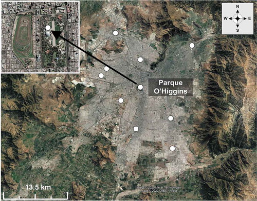
The monitor was located about 400 m west from a major highway, and about 580 m east of a horse racetrak and 440 south of a large street (Blanco Encalada), there are several small shops outside the park. Because the station is far from the highway, the horse racetrack and the street, emissions from these large sources can be considered part of the normal activity of the city. The station is located in the geometrical center of the city; it has several instruments that measure CO, CO₂, continuous PM₁₀ and PM_2.5, NO_x, SO₂, O₃, and meteorological parameters (wind speed [WS] and direction, temperature, relative humidity). This station is part of the Monitoring Network (Sinca 1997) from the Ministry of the Environment and has been in operation since 1988 and its data is publicly available on the web page. Daily rainfall data was obtained from the Chilean Meteorological Service (DMC 2020) from 1998 until 2020, which is also publicly available.

Data collection

A Dichotomous Sampler (Andersen Instruments, Inc., now a Thermo Instruments Systems, Inc. subsidiary) was used to collect 24-hour PM_2.5 (fine) and PM_10-2.5 (coarse) samples. PM₁₀ was calculated as the sum of coarse and fine particle concentrations. The instrument was located inside a temperature-controlled container with the sample inlet at 3 m height. The sampling was performed from midnight to midnight with a daily frequency in the fall/winter season (April–September) and every two days in the spring/summer season (October–March). The total flow rate was 16.7 l/min, with a major flow of 15 l/min for fine particles (PM_2.5) and a minor flow of 1.7 L/min for large particles (PM_10-2.5). Particle concentrations were determined gravimetrically using an electronic microbalance with a resolution of 0.001 mg. Both blank and field filter samples were conditioned following national laboratory protocols at a constant temperature and RH (20–45% RH and 15–30 °C) for at least 24 hr before being weighed. X-ray fluorescence (XRF) analysis was carried out at two different laboratories. Filters from 1998 to 2010 were analyzed at Desert Research Institute (DRI) and the more recent filters where analyzed at Department of Environmental Health, Harvard T.H. Chan School of Public Health. The filters are collected by and belong to the Ministry of the Environment. To minimize laboratory costs, they have focused historical XRF analysis on the fine fraction of the filters. The decontamination politics of Santiago de Chile were imposed mainly to control fine particles. Then, a smaller subset of coarse filters was available for XRF analysis. For the whole period, 1839 PM_2.5 and 773 PM_10-2.5 filter samples were available for XRF analysis, giving from 3 to 15 and 3 to 13 filters/month for fine and coarse fraction, respectively. Six blank filters with XRF analysis were included between years 2014 and 2018. Concentration values below its laboratory uncertainty (two times the uncertainty corresponds to the lower detection limit [LOD] for each sample and element) were excluded from the dataset. Elemental concentrations were not blank corrected because the laboratory uncertainty of the blanks was higher than filters with sample. Following Sax et al. (2007), a “year period” was defined from April of one year until March of the following year. Seasons (fall/winter or spring summer) with less than 65% of elemental results were excluded from the dataset. Twenty-three elements were above this minimum for PM_2.5 and 22 elements for PM_10-2.5 and were considered for the statistical analysis.

Regression analysis

In order to study the influence of the meteorological variables in the evolution of the particulate material, a multivariate linear regression analysis (Chaloulakou et al. 2003; Koutrakis et al. 2005) was applied to the years 1998–2018 to fine (PM_2.5) and coarse (PM_10-2.5) fraction of PM. Model performance was assessed using standard errors of the estimated slopes, and p-values. This analysis is used to describe the relationship between a response variable “Y” with one or more categorical predictor variables X₁, X₂ … X_n. In this case, PM concentrations were log transformed, and Log(PM) was used as “Y” variable, which was regressed against following categorical variables: “year,” “month,” “weekday,” and meteorological measurements (“temperature,” “relative humidity,” and “wind speed”). Continuous data were converted to categorical variables to capture nonlinear relationships over each variable’s range (the variables and its ranges were selected following Koutrakis et al. 2005). Meteorological variables were dichotomized or trichotomized using the following ranges:

• wind speed: WS < 0.8 m/s, 0.8 < WS < 1.6 m/s, WS > 1.6 m/s

• relative humidity: RH > 80% and RH < 80%

• temperature: T < 20°C and T > 20°C

• rain: day with rainfall, day without rainfall.

These ranges are as follows:

(1) $log\left(PM\right)=\alpha +\mathrm{\Sigma }{\beta }_{yea{r}_j}\ast yea{r}_j+\mathrm{\Sigma }{\beta }_{mont{h}_k}\ast mont{h}_k+\mathrm{\Sigma }{\beta }_{weekda{y}_l}\ast weekda{y}_l+\mathrm{\Sigma }{\beta }_{windspee{d}_m}\ast windspee{d}_m+\mathrm{\Sigma }{\beta }_{temperatur{e}_n}\ast temperatur{e}_n+\mathrm{\Sigma }{\beta }_{relativehumidit{y}_p}\ast relativehumidit{y}_p+\mathrm{\Sigma }{\beta }_{rai{n}_q}\ast rai{n}_q+\epsilon$(1)

where $\alpha$ is the regression intercept, ε is the error term, and ${\beta }_{yea{r}_j},{\beta }_{mont{h}_k},{\beta }_{weekda{y}_l},{\beta }_{windspee{d}_m},{\beta }_{temperatur{e}_n},{\beta }_{relativehumidit{y}_p},\text{break}{\beta }_{rai{n}_q,}$ are the coefficients of categorical variables. The “year” variable is defined as measurements collected from the period January to December. The rest of categorical variables are expressed as “month” (k = 1 to 12), “weekday” (l = 1 to 7), “wind speed” (m = 1 to 3), “temperature” (n = 1 to 2), “relative humidity” (p = 1 to 2), and “rain” (p = 1 to 2). The strength of the association was determined by the significance of the slope t-values. This multivariate regression model allows explaining the variability of the concentration of the particulate material as a function of the effect of different predictive categorical variables, using the Concentration Impact Factor (CIF) of a variable i, which is detailed below.

Based on Equation (1)(1) $log\left(PM\right)=\alpha +\mathrm{\Sigma }{\beta }_{yea{r}_j}\ast yea{r}_j+\mathrm{\Sigma }{\beta }_{mont{h}_k}\ast mont{h}_k+\mathrm{\Sigma }{\beta }_{weekda{y}_l}\ast weekda{y}_l+\mathrm{\Sigma }{\beta }_{windspee{d}_m}\ast windspee{d}_m+\mathrm{\Sigma }{\beta }_{temperatur{e}_n}\ast temperatur{e}_n+\mathrm{\Sigma }{\beta }_{relativehumidit{y}_p}\ast relativehumidit{y}_p+\mathrm{\Sigma }{\beta }_{rai{n}_q}\ast rai{n}_q+\epsilon$(1) , particle concentrations can be expressed as the product of the exponential terms:

(2) $PM=exp\left[\alpha \right]\ast exp\left[\begin{array}{c}\mathrm{\Sigma }{\beta }_{perio{d}_j}\ast perio{d}_j+\mathrm{\Sigma }{\beta }_{mont{h}_k}\\ \ast mont{h}_k+\mathrm{\Sigma }{\beta }_{weekda{y}_l}\ast weekda{y}_l\\ +\mathrm{\Sigma }{\beta }_{windspee{d}_m}\ast windspee{d}_m\\ +\mathrm{\Sigma }{\beta }_{temperatur{e}_n}\ast temperatur{e}_n\\ +\mathrm{\Sigma }{\beta }_{relativehumidit{y}_p}\ast relativehumidit{y}_p\\ +\mathrm{\Sigma }{\beta }_{rai{n}_q}\ast rai{n}_q\end{array}\right]\ast \mathrm{e}\mathrm{x}\mathrm{p}\left[\epsilon \right]$(2)

which can be simplified to

$PM=I\ast f_{perio{d}_j}\ast f_{mont{h}_k}\ast f_{weekda{y}_l}\ast f_{windspee{d}_m}\ast f_{temperatur{e}_n}\ast f_{relativehumidit{y}_p}\ast f_{rai{n}_q}$

.

CIF of a variable “I” is defined as $CIF=f_{variabl{e}_j}=\text{break}exp\left[\mathrm{\Sigma }{\beta }_{variabl{e}_j}\ast variabl{e}_j\right]$. For each of the categorical variables, a reference level was set, with subsequent effects calculated relative to that reference variable. For this analysis, Monday, January, and year 1998 were set as the reference variables for “weekday,” “month,” and “year,” respectively. For the meteorological variables, the lowest ranges were used as the reference for the corresponding group.

The CIF for the intercept, I = e^α, corresponds to the average concentration at the reference level. For the other variables, a regression coefficient of 0 equals a CIF of 1, meaning that the variable has no effect. Conversely, a CIF greater than 1 represents a greater concentration of PM, relative to the reference point, and a value less than 1 represents a concentration that is lower relative to the reference. It is worth mentioning that the CIFs are relative indices, not absolute. In other words, the CIF values provided by the model are values relative to reference levels defined a priori during the regression analysis. Therefore, the CIFs are interpreted as increases or decreases in concentration attributed to the variation of an explanatory variable, with respect to the defined reference level. The significance of the association was determined by the p-values of the estimates. CIF’s were calculated for each element/mass concentration against categorical variables. For each pollutant, a multiple regression analysis was performed.

Cluster and heatmap analysis

For the heatmap analysis of the elements (Babicki et al. 2016), data was processed as follows. Daily concentrations for elements were considered valid if the concentration value surpassed its associated uncertainty. For each valid daily concentration, the percentage of contribution of each element to either fine or coarse fractions was calculated. Median of daily percentage of contribution for each element for given year was calculated, and a valid yearly percentage of contribution value for each element was considered when it comprised 50% or more valid daily values separately. For all years analyzed (1998–2018), the median and standard deviation of annual percentage of contribution values was calculated. Only those elements that had three or more valid annual percentage of contribution values were included in the heatmaps. Row-Z score was calculated for each element for a given year as the number of standard deviations from the median. Higher than the median values were reported as positive in red color, while values below the median were reported as negative in green color. Hierarchical clustering was performed using average linkage clustering method and Euclidean distances for a given fraction. The analysis was performed using the online visualization tool Heatmapper (Babicki et al. 2016).

Results

Particle matter (PM) analysis

A summary of the gravimetric results for PM_2.5, PM₁₀, and PM_10-2.5 is presented in Figure 2 for the years 1988–2018. As mentioned before, Parque O’Higgins station is far from direct emission sources; however, during 1993, there was a spike in PM₁₀ due to construction work, and thus data from that period was not considered in the regression analysis. Figure 2a shows that both PM₁₀ and PM_10-2.5 have had an almost continuous decrease since 1988. As mentioned in the introduction, there have been several measures implemented to reduce emissions that are mentioned in previous studies (Jhun et al. 2013; Jorquera and Barraza 2012; Koutrakis et al. 2005; Moreno et al. 2010; Sax et al. 2007). PM_2.5 concentration has decreased from 68.3 in 1988 to 27.6 μg/m³ in 2018 (60.4%), PM₁₀ decreased from 112.4 to 72.6 μg/m³ in 2018 (35.4%), but PM_10-2.5 remained constant from 1988 until 2018 (with several fluctuations in those years). However, annual average concentration of PM₁₀ still exceeds the Chilean and WHO standards of 50 and 20 μg/m³ respectively. For PM_2.5 the Chilean and WHO annual standards of 20 and 10 μg/m³ are also exceeded.

Figure 2. (a) Annual PM₁₀ and PM_2.5 concentrations. (b) Annual PM_2.5 concentrations for fall/winter and spring/summer. (c) Annual PM_10-2.5 and PM_2.5 concentrations. (d) Annual PM_10-2.5 concentrations for fall/winter and spring/summer

If only the last 8 years are considered (2011–2018), a leveling off can be observed in PM₁₀ and PM_2.5. A Mann--Kendall trend test analysis (EPA 2016; Mann 1945) with 95% confidence indicates that there is insufficient evidence of an increase in PM_2.5 or PM₁₀. However, for the last 8 years, it indicates a change in the tendency that is important to analyze in order to find the causes. Figure 2b shows the PM_2.5 curve separated for fall/winter (April–September) and spring/summer (October–March) periods. The fall/winter period seems to have a larger decrease, but the relative change (68% decrease) from 1998 until 2019 is the same for both periods. The fall/winter period seems to have a tendency to increase in the last 8 years while the spring/summer concentration seems to be constant (Figure 2a), but a Mann--Kendall trend test for either period does not indicate evidence for increase or decrease. The figure also shows a strong seasonal pattern, with fall/winter mean concentrations 2–3 times higher than spring/summer. Figure 2c shows the annual PM_10-2.5 and PM_2.5 concentration, an interesting feature that can be seen is that the coarse fraction has not changed much since 1988. This lack change has also been pointed out by Koutrakis et al. (2005), and it is probably due to the origin of this fraction. It is well known that coarse particles are mostly from natural origin, generated by mechanical processes: wind, vibration, resuspension from roads, mechanical wear, etc. Santiago’s climate is semi-arid with an average of 261.6 mm of rainfall per year, mainly during winter. During summer, RH is very low (20%–40%), with clear skies and high temperatures during the day. These circumstances promote soil dryness and resuspension of dust facilitated by wind or vehicular traffic (Amato et al. 2009; de la Paz et al. 2015; Hussein et al. 2008). However, high temperatures also enhance vertical dispersion (Gramsch et al. 2014), which tends to decrease concentrations; thus there is a competing effect on pollution. It has to be noted that, because there is scarce rainfall in winter, the ground is dry most of the time, setting the conditions for coarse PM generation. Figure 2d shows the coarse fraction separated by season. In contrast to the fine fraction, there is almost no difference between the spring/summer or fall/winter seasons which indicates that rainfall does not have a large influence preventing the generation of coarse PM.

In the past 9 years, there has been a persistent drought in Chile, with a reduction in rainfall up to 45% in some areas of central Chile (Garreaud et al. 2017). In a semi-arid region, like South America (latitude 30º–38º south), it is normal to have droughts that last 1–2 years, but the present drought has lasted for more than 9 years, which is rare. On the other hand, mean temperatures have also increased in the same period. Figure 3 shows rainfall and temperature measured by the Chilean Meteorological Service (DMC 2020) in the Quinta Normal station in downtown Santiago de Chile. The increase in temperature in these 21 years is evident and a Mann--Kendall statistical analysis (EPA 2016) gives a significant increase with 95% confidence and a slope of 0.0203 C/year. Rainfall has a very large annual variability, and the trend is harder to see. However, as shown in the inset of Figure 3, the average of the last 9 years (2011–2019) is 192.2 mm/year, and the average for the previous 9 years (2002–2010) is 343.3 mm/year. A t-Student test between these two periods indicates that the 2002–2010 average is statistically larger than the 2011–2019 average with a 95% confidence.

Figure 3. (a) Rainfall and (b) temperature measured in downtown Santiago from 1998 to 2018. The inset shows the average rainfall of the last and previous 9 years

Regression analysis for PM_2.5 and PM_10-2.5

For this study, multivariate regressions were performed using continuous data from PM₁₀ and PM_2.5 depending on the meteorological variables (humidity, temperature, wind speed, and rainfall), measurement season (winter or summer), day of the week (Monday--Sunday), month of the year (January–December), and year of measurement (1998–2018) in order to observe trends in concentration.

It is worth mentioning that the CIFs are relative indices and the values provided by the model are relative to reference levels defined a priori during the regression analysis. Therefore, the CIFs are interpreted as increases or decreases in concentration attributed to the variation of an explanatory variable, with respect to the defined reference level. The interpretation of this logical variable in the regression analysis results differs from that of the regular multiple regression analysis. The results should be interpreted by categorical variable sets, since each set originates from one continuous or character parameter. Chaloulakou et al. (2003) included a discussion about this, and indicated that creating independent categorical variables make them harder to be correlated. The original objective of the statistical analysis (Chaloulakou et al. 2003) was to identify meteorological or time period parameters that can be used to predict particle levels (prognostic model); however, in later works (Koutrakis et al. 2005; Sax et al. 2007) and in this work, it is used to estimate the relative impact of meteorological/categorical variables included in statistical model.

The “week effect” of the CIF analysis between years 1998 and 2018 is shown in Figure 4a for PM_10-2.5 and PM_2.5. The error bars in the figure corresponds to the standard error in the model and are relatively small (the error and p-values are in the Supplementary Information). It considers as reference the average concentration levels on Monday, that is, the CIFs indicate if the values increase or decrease with respect to the average measurements on Mondays. The factor is higher on weekdays (except Monday) and it is lower on Sunday, revealing that it is mainly related to the anthropogenic activities of the city. PM_10-2.5 has a slightly stronger variation than PM_2.5 changing from 1.11 on Friday to 0.85 on Sunday, which is a 23% decrease; on the other hand, PM_2.5 decreases from 1.15 to 1 reaching a 13% reduction. The weekly variation in both mass fractions can be understood because in a city a large portion of PM_2.5 is emitted by vehicles (Usach Emission inventory 2014) and other anthropogenic activities. Weekdays and Saturday showed higher concentrations of PM_2.5 than Sunday; however, for PM10-2.5, Saturday and Sunday are lower than weekdays. Coarse particles are generated by wind or vehicle-promoted resuspension which is also related to traffic in the city. Querol et al. (2004) found that in several European cities exhaust and non-exhaust sources contributed approximately equal amounts to total traffic-related emissions of particulate matter. A similar study in Berlin (Lenschow et al. 2001) demonstrated that around half of the observed increase of PM₁₀ at roadside above the urban background could be attributed to resuspension of road dust particles. A recent review (Penkała, Ogrodnik, and Rogula-Kozłowska 2018) also found that road surface abrasion remains an important PM source.

Figure 4. (a) Concentration impact factor for weekdays for PM_2.5 and PM_10–2.5, (b) Monthly concentration impact factors. (c) Wind speed (WS, m/s), temperature (T, C), relative humidity (RH, %), and rain (Pp) CIFs. The error bars are the standard error

The “month effect” of the CIF analysis is shown in Figure 4b and has a clear distinction between coarse and fine PM, with the reference concentration level chosen to be January. The regression analysis for PM_2.5 has a large variation along the year, with a minimum of 0.89 in November (spring) and a maximum of 3.35 in July (winter), i.e., a factor of 3.8 increase between these months. The error and p-values (included in the Supplementary Information) for the “month effect” are all lower than 0.05 indicating that the increase during winter is statistically significant. As mentioned previously (Gramsch et al. 2006; Koutrakis et al. 2005), the large difference is related to a reduced mixing volume because of frequent temperature inversions (Gramsch et al. 2014) and emission sources that are not present in summer or spring, like space heating. Previous studies have shown that biomass burning contribution to PM_2.5 is significant in winter and on episode days (Carbone et al., 2013; Gramsch et al. 2016; Tagle et al. 2018). It has to be noted that in this calculation, the wind, temperature and humidity effects have been taken out and the variation seen in Figure 4b is not due to temperature, humidity, or wind. The large difference indicates that the smaller mixing layer and the added pollution sources during winter are a determinant factor in the high PM_2.5 levels observed.

The monthly impact factor for PM_10-2.5 has a modest variation during the year (Figure 4b), being slightly higher in March and April. As mentioned before, this fraction is related to larger particles being resuspended by wind, mechanical processes, vehicular traffic, etc. In turn, it also depends on WS and the conditions of the ground. If the ground is damp, there is going to be less dust resuspension, which seems to be the case indicated by the PM_10-2.5 curve in Figure 4b. In Santiago de Chile, rainfall occurs only during the winter months (May–August) and summer is usually very hot and dry; in addition, the WS increases during summer. These conditions promote resuspension of PM during summer months.

The WS, temperature, RH, and rainfall impact factors are shown in Figure 4c. The CIFs values decrease from 1 to 0.69 for PM_2.5 with higher WSs, which is associated with increased horizontal ventilation in Santiago’s valley. However, there is no statistical difference for WS > 0.8 m/s for either fraction. For temperature, there is also a decrease in the CIFs when temperature is higher than 20  C for both PM_2.5 and PM_10-2.5 associated with increased vertical ventilation in the valley. Considering the error bars in Figure 4c, for PM_10-2.5 the decrease in the CIF when temperature is > 20  C is non-negligible. From this data, it can be seen that the increase in temperature in the last 30 years has not directly contributed to an increase in concentrations. The p-values for WS, temperature, and RH are all lower than 0.05 for both fractions. The effect of RH on PM_2.5 and PM_10-2.5 CIFs has an interesting feature. A large increase occurs from 1 to 1.36 in the CIF for PM_10-2.5 when the RH is lower than 80%, which could be associated to higher resuspension of PM. In contrast, the CIF for PM_2.5 exhibits a negligible association with low humidity. The rain CIF also has a smaller decrease for PM_2.5 than PM_10-2.5. Both CIFs seem to indicate that there is more resuspension for PM_10-2.5 than PM_2.5. As mentioned in the previous section, there has been a persistent drought in Chile since 2011. Concentration impact factor for rainfall is shown in Figure 4c and indicates a decrease from 1 to 0.62 for PM_10-2.5 and a decrease from 1 to 0.82 for PM_2.5 which can be understood because rain inhibits the resuspension of PM and removes airborne PM through the wet deposition process (Seinfeld and Pandis 1998). As shown in Figure 4c, these effects are more pronounced with coarse PM than fine PM. The p-values (included in the Supplementary Information) for days with rain for PM_10-2.5 is less than 0.01 and p = .06 for PM_2.5. The CIF analysis shown in Figure 4c indicates that particle concentrations increase when rainfall decrease which is a confirmation that the latest drought in Chile has an effect on the PM concentration leveling off.

The “year effect” of the CIF analysis considers as reference concentration levels the measurements made in 1998 for PM_2.5 and PM_10-2.5. Figure 5 shows a sustained decrease of the CIFs for both fractions for most of the period 1998–2018. However, a change in the trend can also be seen. The decrease in PM_10-2.5 is 69% from 1998 to 2010 and 62% for PM_2.5 in the same period. As mentioned in previous studies (Jorquera and Barraza 2012; Koutrakis et al. 2005; Moreno et al. 2010; Sax et al. 2007), this decrease seem to indicate that the decontamination plans in the Santiago metropolitan area have been effective in reducing coarse and fine PM. A Mann--Kendall trend test (EPA 2016; Mann 1945) with 95% confidence indicates that there is a statistically significant evidence of a decreasing trend for PM_2.5 and PM_10-2.5 CIFs between 1998 and 2010. The straight lines in Figure 5 are ordinary least squares (OLS) fits to the data.

Figure 5. Concentration impact factor for the year effect for PM_2.5 and PM_10-2.5. The straight lines indicate an OLS regression lines to the data for each period. The error bars are the standard error

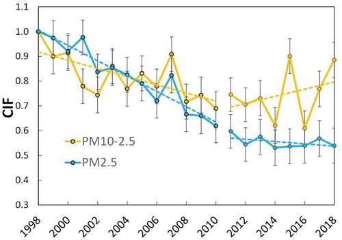
However, from 2011 until 2018, there seems to be a change in the tendency for PM_2.5 and PM_10-2.5 that correlates with the extended drought in central Chile. The CIF values in Figure 5 tend to be either increasing or constant, indicating that new factors affect the concentrations. In this case, a Mann--Kendall trend test (EPA 2016) with 95% confidence indicates that there is insufficient evidence to identify an increase or decrease in PM_2.5 or PM_10-2.5 CIFs between 1998 and 2010. The regression line in Figure 5 for PM_10-2.5 has a positive slope between 2011 and 2018 and the PM_2.5 regression has a negative slope less sharp than that found in the preceding (1998–2010), indicating that the change in tendency could be due to relative changes in coarse PM sources. As mentioned before, the last 9 years have had less rain and higher temperatures than before, as a consequence that the ground would be drier and resuspension of coarse PM would be easier.

Cluster analysis for the chemical elements

An analysis of the chemical elements in PM_2.5 and PM_10-2.5 has been performed in an attempt to find the sources contributing to the changes in the trend. The concentrations of the elements, measured with XFR include from Z = 11 (Na) to 82 (Pb) and the concentrations are of the order of a few ng/m³.

Similarities in the temporal variability of the concentration of the elements (fine or coarse fraction) reflect affinities between them. The quantification of this degree of affinity is done using the “cluster analysis method” (Everitt 1993). The elements were grouped by proximity using a distance parameter. In turn, the groups that showed different degrees of closeness were grouped hierarchically. Hierarchical clustering was performed using average linkage clustering method and Euclidean distances for a given fraction. The results are shown in Figure 6a for PM_2.5 and Figure 6b for PM_10-2.5. It has to be noted that PM_2.5 and PM_10-2.5 groups have different elements because they come from different sources (EPA SPECIATE 2020). The blue line in the figure shows the cut point for the groups.

Figure 6. Hierarchical clustering and heat map for the relative contribution of elements in (a) PM_2.5 and (b) PM_10-2.5. The colors (Row Z Score) represent the number of standard deviations over (yellow) or below (blue) the median for each element

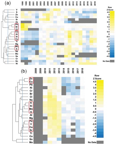
For PM_2.5, the groups found are associated with crustal elements (Ca, Al, Si, Fe), related to vehicular combustion (Pb, Br, Cl) (Jorquera and Barraza 2012; Marmur, Mulholland, and Russell 2007), or resuspension of enriched road dust (Young et al. 2002), and a third group that also may be associated to soil dust or wood burning (K, Mn) (Jorquera and Barraza 2012; Marmur, Mulholland, and Russell 2007).

In the PM_10-2.5 crustal elements, three groups have been selected which are: Zn and Cu; K, Si, Mn, and S; Fe, V, Ca, and Sr. In this selection, Zn and Cu are very close and it has been associated to brake wear (Garg et al. 2000; Lough et al. 2005). It has to be noted the Zn and Cu are also grouped in the cluster analysis of PM_2.5, but the association is not as strong as in PM_10-2.5, which also points to the break wear source because it generates large particles. The other groups probably have mixed origin (K, Si, Mn, S), (Fe, V, Ca, Sr, Ti) because they have elements from the soil, industry, vehicles, etc. Figure 6a shows that for the crustal source in fine PM (Ca, Al, Si, and Fe) there is a relative increase from 2010–2011 matching with the beginning of rainfall reduction. Elements related to vehicular combustion (Pb, Br, Cl) showed a consistent rapid decrease from 1998–2001 and a maintenance in their relative contribution to the fine fraction afterward. For the coarse fraction (Figure 6b), all elements followed a similar pattern showing a decrease in their relative contribution from 2013–2014. However, results before 2010 were not available; relevant trends including the period preceding the rainfall scarcity could not be identified for this fraction.

Concentration impact factor for elements in PM_2.5

Multivariate regressions were calculated for all elements present in PM_2.5 and PM_10-2.5 filters from 1998 until 2018. As before, the analysis allowed removing the influence of meteorological variables (WS, temperature, humidity, and rain) from the data in order to observe trends in concentration.

As mentioned before, the concentration of chemical elements is a very small fraction of the total PM mass, and small errors in the measurements can generate large changes in the element concentration. Therefore, there is a large variability in the year-to-year concentration. As shown in Figure 5, there is a clear change in tendency in PM concentration. Before the year 2010, there was a decrease in concentration which was confirmed with a Mann--Kendall test. After the year 2010, PM concentrations have stabilized, and thus, an analysis of the chemical elements in PM_2.5 was done for years 2011–2018. Cluster analysis (Figure 6a) shows the groups that are more strongly related. The first group represents the crustal elements Si, Al, Ca, and Fe, the second group is Pb, Br, and Cl, and the third group is Mn and K. The CIF results for these elements are plotted in Figure 7 and the error bars correspond to the standard deviation. Figure 7a shows that for most crustal elements the CIF has remained stable (the errors and p-values are included in the Supplementary Information), which is consistent with what was observed for PM_2.5 in Figure 5. Figure 7b shows the monthly CIF for the same elements, and two tendencies can be seen: Al and Si remain stable during the year, but Ca and Fe have an increase during winter months. This increase is very similar to the increase that PM_2.5 has during winter months (Koutrakis et al. 2005; Jorquera, Palma, and Tapia 2000; and Figure 4b). Because PM_2.5 is mainly generated by anthropogenic sources (Seinfeld and Pandis 1998), the Fe fraction contained in PM_2.5 is likely coming from anthropogenic sources. Ca also shows an increase during winter, but not as high as Fe; thus, it is also likely that these elements are also from anthropogenic origin. During winter, poor air mass mixing favors the accumulation of fine particles increasing its concentration (Koutrakis et al. 2005). Fe may be generated in agricultural practices (Prospero et al. 2002), biomass burning (Fu et al. 2014; Guieu et al. 2005), or combustion emissions (Chuang et al. 2005; Fu et al. 2012). Ca may be generated by road dust because of the abundance of alkaline materials in road coverings (Gillette et al. 1992), and thus, Ca can be generated by vehicle traffic. Al and Si do not have an increase during winter, and the monthly profile is similar to the PM_10-2.5 profile (see Figure 4b and Koutrakis et al. 2005).

Figure 7. Yearly and monthly CIFs for the clustering groups in PM2.5. (a) yearly CIF for elements associated to the earth crust, (b) monthly CIF for elements associated to the earth crust, (c) yearly and (d) monthly CIFs for elements associated transport or wood burning, (e) yearly an d (f) monthly CIFs for elements associated to soil dust. The error bars are the standard error

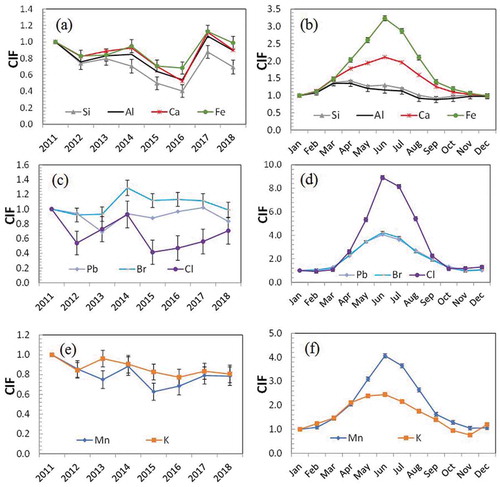
The second group of elements in PM_2.5 was composed of Pb, Br, and Cl, which can be associated to transport or wood burning. For this group, the CIF also has remained stable (Figure 7c), which is similar to what was observed for PM_2.5. Pb and Br were used in gasoline as anti-knock additive to increase the octane number until 2001 (Ley Chile 2001). Pb and Br removal from the gasoline lead to a significant decrease in concentrations. Pb decreased from 700 ng/m³ in the winter of 1998 to 30 ng/m³ in the winter of 2018. Br decreased from 250 ng/m³ in the winter of 1998 to 11 ng/m³ in the winter of 2018 (Sax et al. 2007). However, Br and Pb are still present in PM probably because of contaminated dust or emissions from small vehicle repair shops, metal shops, and tire and brake wear (Lough et al. 2005; Wahlin, Berkowicz, and Palmgren 2006). Cl is used to treat drinkable water in Santiago de Chile, and it is probably disseminated in the whole city, in particular over the roads and can be resuspended by vehicle traffic. However, Cl has a strong monthly dependence (Figure 7d), increasing during winter; thus, Cl is probably coming from wood burning (Marmur, Mulholland, and Russell 2007). This group has probably a mixed origin.

The third group is composed of Mn and K, which seem to have decreased in the 2011–2018 period. For K, a Mann--Kendall trend test gives a statistically significant evidence of a decreasing trend with 95% confidence and p = .016. For Mn, there is no evidence of a decrease with 95% confidence.

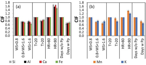
The influence of meteorological parameters on the particle concentrations is shown in Figure 8 and indicates a strong dependence with these variables (the errors and p-values are included in the Supplementary information). For all elements, the WS CIF decreases from 1 to ~ 0.8 for speeds greater than 0.8 m/s, with no further decrease for larger speeds. For temperatures greater than 20  C, there is also a decrease in all CIFs, which is non-negligible and could be related to greater vertical dispersion (Gramsch et al. 2014). The RH also has a strong influence on the concentrations, with lower RHs the CIFs increases, which is related to less condensation and agglomeration of particles and less decay to the ground.

Figure 8. Wind speed (WS, m/s), temperature (T, C), relative humidity (RH, %), and rain (Pp) CIFs (a) for the crustal elements, (b) for Mn and K. The error bars are the standard error

Considering the error bars in Figure 8, it can be seen that for all elements, there is no change in concentration from 2011 to 2018, which is consistent with the trend in PM_2.5 (Figure 5) for the same period. A recent publication (Menares et al. 2020) found an increase in secondary aerosols from 2001 to 2018 due to the growth of NO₂ and O₃. Secondary aerosols cannot be measured using XRF techniques (Seinfeld and Pandis 1998) and could explain the stability observed in PM_2.5.

Concentration impact factor for elements in PM_10-2.5

The main groups that are formed with the elements present in PM_10-2.5 are Zn and Cu; S, Mn, K, and Si; Fe, V, Ca, and Sr (Figure 6b). XRF data for this fraction was only available from 2009–2018. The CIF results for these elements are shown in Figure 9, and the error bars correspond to the standard deviation (the errors and p-values are included in the Supplementary Information). For clarity in the figure, not all error bars are plotted.

Figure 9. Yearly and monthly CIFs for the clustering groups in PM10-2.5. (a) yearly CIF for elements associated to brake wear, (b) monthly CIF for elements associated to the brake wear, (c) yearly and (d) monthly CIF for elements associated to the earth crust , (e) yearly and (f) monthly CIF for another group of elements associated to earth crust. The error bars are the standard error

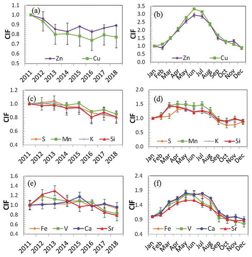
The first group in PM_10-2.5 is formed by Zn and Cu. Figure 9a shows that both elements seem to decrease and a Mann--Kendall test shows evidence of a decrease for Cu with 95% confidence (p = .007) but not for Zn (p = .119). These elements have a stronger monthly dependence (Figure 9b), which is an indication that they have anthropogenic origin. The Zn and Cu group could be related to brake wear (Garg et al. 2000; Lough et al. 2005).

The second group in PM_10-2.5 has crustal elements, formed by K, Si, Mn, and S. The yearly CIFs results for the crustal elements are shown in Figure 9c and the monthly CIFs are shown in Figure 9d. All elements show a decrease in the CIFs from 2011 to 2018, and a Mann--Kendall test shows statistically significant evidence of a decreasing trend with 95% confidence for K (p = .007), Si (p = .007), Mn (p = .016), and S (p = .02). S is generated by multiple sources, most of them emit only fine particles, and thus the S present in the PM_10-2.5 fraction originates probably from resuspended contaminated dust. Si, Mn, and K are also known to come from the earth crust (Jorquera and Barraza 2012; Marmur, Mulholland, and Russell 2007). All these elements have a weak dependence with the month of the year, which is consistent with the monthly CIF of PM_10-2.5 in Figure 4b. This group probably is mostly associated to clean or contaminated dust resuspension.

The third group in PM_10-2.5 is formed by Fe, V, Ca, and Sr. The yearly CIFs for these elements is shown in Figure 9e. For these elements, a Mann--Kendall test does not show a statistically significant evidence of a decrease. These elements have a stronger monthly dependence (Figure 9f) than the other group with crustal elements (S, Mn, K, Si), which indicate that they have some anthropogenic influence. Fe and Ca are known to come from the soil (EPA SPECIATE 2020; Jorquera and Barraza 2012; Marmur, Mulholland, and Russell 2007). Sr and V are not commonly found in soil samples (Chow et al. 2004; Marmur, Mulholland, and Russell 2007), but in the central area of Chile, Hedberg et al. (2004), found these metals as part of the soil samples.

The influence of meteorological variables on the concentration of the selected elements is shown in Figure 10 (other the other elements show similar influence). As before, the CIF for all elements always decrease with WS (Figure 10a) decrease with higher temperatures and increase with lower RH. For instance, Si changes from a CIF of 1.0 at WS < 0.8 m/s to 0.72 at WS > 1.6 m/s, Al changes from a CIF of 1.0 at WS < 0.8 m/s to 0.70 at WS > 1.6 m/s. For Si, the CIF for temperature decreases from 1.0 to 0.82, with an error of 0.04 (all errors and p-values are included in the Supplementary Information). The influence of rain is also clear in all elements; the CIFs always decrease when there is precipitation, which confirms the hypothesis that the long drought in central Chile has had an influence in the change of tendency (stability) of PM_10-2.5 and PM_2.5 concentrations.

Figure 10. Wind speed (WS, m/s), temperature (T, C), relative humidity (RH, %), and rain (Pp) CIFs (a) for the crustal elements in PM_10-2.5, (b) for Na, Cl, and S. The error bars are the standard error

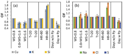
There are three elements that behave different with WS and temperature; these are S, Na and Cl. As shown in Figure 10a, the CIF for Cl changes from 1.0 at WS < 0.8 m/s to 1.2 at WS > 1.6 m/s and the CIF for Na changes from 1.0 at WS < 0.8 m/s to 1.06 at WS > 1.6 m/s. The CIF for Na does not change with temperatures > 20 C and the CIF for Cl increases to 1.03. The most probable motive for this difference is that Na and Cl come from the sea-–which is located about 100 km toward the west–-in the form of common salt (NaCl) and only comes when the WS is higher than 1.6 m/s and high temperatures. In Santiago’s valley WSs are higher during spring and summer, which is from September through February (Gramsch et al. 2006). S shows a similar behavior with high WSs and higher temperature, which indicates that the S found in PM_10-2.5 is most likely coming from the sea or sources located near the sea.

For PM_10-2.5 there are two groups related to crustal elements, one of them decreases (S, Mn, K, and Si) and the other remains stable (Fe, V, Ca, and Sr). Because the chemical elements are a small fraction of the total PM mass, it is hard to determine which group is dominant. The stability observed in PM_10-2.5 in the last 8 years (Figure 5) may be related to other components (EC, OC, Cl⁻, NO₃⁻, NH₄⁺) (Rubio et al. 2018) present in this fraction. Barraza et al. (2017), performed source apportionment from 1998 to 2013 and found that only the urban dust source had increased, while others decreased or remained stable, which is consistent with the stability found in this work for PM_10-2.5. There is no trend analysis of the chemical components because measurements are expensive and only short term campaigns have been performed in Santiago de Chile (Jorquera and Barraza 2012; Rubio et al. 2018; Villalobos et al. 2015)

Conclusion

PM_2.5 and PM_10-2.5 fractions have had a continuous decrease since 1988 mostly due to several policy control measures carried out over several decades. Data shows that PM_2.5 has decreased from 68.3 in 1988 to 27.6 μg/m³ in 2018 (60.4%), and PM₁₀ decreased from 112.4 to 72.6 μg/m³ (35.4%) in the same period. Thus, it seems that control policies have had an impact in the reduction of PM_10-2.5 and PM_2.5 from 1998 until 2010. If only the last 8 years are considered (2011– 2018), a leveling off can be observed in PM_10-2.5 and PM_2.5 which points to a change in the tendency. Part of the reason for this leveling off, could be that in the last 9 years there has been a persistent drought in Chile, with a reduction in rainfall up to 45% in some areas. Cluster analysis has been applied to the elements in the fine and coarse fractions to separate groups of elements that can be associated to a source. The fraction of PM_2.5 associated to the crustal elements (Si, Al, Ca, and Fe) has remained stable in the last 8 years and a fraction associated to anthropogenic sources (traffic, wood burning) has also remained stable in the same period. This phenomenon can be partly ascribed to lower amount of rain during the last 8 years that keep the ground dry allowing easier resuspension of dust due to wind or vehicular traffic. Higher temperatures in the last 30 years have not contributed directly to a reduction of concentration.

For PM_10-2.5 one fraction associated to crustal elements (K, Si, Mn, and S) has decreased in the last 8 years, but another fraction (Fe, V, Ca, and Sr) has remained stable. Thus the leveling off of PM_10-2.5 may be related to other components not analyzed in this work.

Disclosure statement

No potential conflict of interest was reported by the authors.

Supplementary material

Supplemental data for this article can be accessed on the publisher’s website.

Additional information

Funding

This work was supported by Fondecyt project 1151117 and by the Chilean Ministry of the Environment.

Notes on contributors

Ernesto Gramsch

Ernesto Gramsch is a professor at the Physics Department of the University of Santiago de Chile, Santiago, Chile.

Pedro Oyola

Pedro Oyola is the director at Mario Molina Center for Strategic Studies of Energy and Environment, Santiago, Chile.

Felipe Reyes

Felipe Reyes, is a research associates at Mario Molina Center for Strategic Studies of Energy and Environment, Santiago, Chile.

Francisca Rojas

Francisca Rojas is a research associates at Airflux Spa, Santiago, Chile.

Andrés Henríquez

Andrés Henríquez is an ORISE postdoctoral fellow at US Environmental Protection Agency, NHEERL/EPHD/CIB, Research Triangle Park, NC, USA.

Choong-Min Kang

Choong-Min Kang is a research scientist at Department of Environmental Health, Harvard TH Chan School of Public Health, Boston, MA, USA.

References

- Amato, F., X. Querol, A. Alastuey, M. Pandolfi, T. Moreno, J. Gracia, and P. Rodriguez. 2009. Evaluating urban PM10 pollution benefit induced by street cleaning activities. Atmos. Environ. 43:4472–80. doi:10.1016/j.atmosenv.2009.06.037.
- Babicki, S., D. Arndt, A. Marcu, Y. Liang, J. R. Grant, A. Maciejewski, and D. S. Wishart. 2016 8. Heatmapper: Web-enabled heat mapping for all. Nucleic Acids Res. 44 (W1):W147–53. doi:10.1093/nar/gkw419.
- Barraza, F., F. Lambert, H. Jorquera, A. M. Villalobos, and L. Gallardo. 2017. Temporal evolution of main ambient PM2.5 sources in Santiago, Chile, from 1998 to 2012
- Barraza, F., F. Lambert, H. Jorquera, A. M. Villalobos, and L. Gallardo. 2017. Temporal evolution of main ambient PM2.5 sources in Santiago, Chile, from 1998 to 2012. Atmos. Chem. Phys. 17:10093–107. doi:10.5194/acp-17-10093-2017.
- Carbone, S., S. Saarikoski, A. Frey, F. Reyes, P. Reyes, M. Castillo, E. Gramsch, P. Oyola, J. Jayne, and D. R. Worsnop. 2013. Chemical characterization of submicron aerosol particles in Santiago de Chile. Aerosol Air Qual. Res. 13:462–73. doi:10.4209/aaqr.2012.10.0261.
- Chaloulakou, A., P. Kassomenos, N. Spyrellis, P. Demokritou, and P. Koutrakis. 2003. Measurements of PM10 and PM2.5 particle concentrations in Athens. Greece. Atmos. Environ. 37:649–60. doi:10.1016/S1352-2310(02)00898-1.
- Chow, J. C., J. G. Watson, H. Kuhns, D. H. Vicken Etyemezian, D. C. Lowenthal, S. D. Kohl, J. P. Engelbrecht, and M. C. Green. 2004. Source profiles for industrial, mobile, and area sources in the big bend regional aerosol visibility and observational study. Chemosphere 54:185–208. doi:10.1016/j.chemosphere.2003.07.004.
- Chuang, P., R. Duvall, M. Shafer, and J. Schauer. 2005. The origin of water soluble particulate iron in the Asian atmospheric outflow. Geophys. Res. Lett. 32. doi:10.1029/2004GL021946.
- de la Paz, D., R. Borge, M. Vedrenne, J. Lumbreras, F. Amato, A. Karanasiou, E. Boldo, and T. Moreno. 2015. Implementation of road dust resuspension in air quality simulations of particulate matter in Madrid (Spain). Front. Environ. Sci. 3:72. doi:10.3389/fenvs.2015.00072.
- DMC. 2020. Accessed June 15, 2020. https://climatologia.meteochile.gob.cl/application.
- EPA. 2016. EPA statistical analysis software. Accessed October 2020. https://www.epa.gov/land-research/proucl-software.
- EPA Regulations. 2020. Regulations, guidance and monitoring plans. Accessed October 2020. https://www.epa.gov/amtic/regulations-guidance-and-monitoring-plans.
- EPA SPECIATE. 2020. repository of organic gas and particulate matter (PM) speciation profiles of air pollution sources. Accessed October 2020. https://www.epa.gov/air-emissions-modeling/speciate.
- Everitt, B. S. 1993. Cluster analysis. 3rd ed. London, UK: Heinemann Education.
- Font, A., L. Guiseppin, M. Blangiardo, V. Ghersi, and G. W. Fuller. 2019. A tale of two cities: Is air pollution improving in Paris and London? Environ. Pollut. 249:1–12. doi:10.1016/j.envpol.2019.01.040.
- Fu, H., J. Lin, G. Shang, W. Dong, V. H. Grassian, G. R. Carmichael, Y. Li, and J. Chen. 2012. Solubility of iron from combustion source particles in acidic media linked to iron speciation. Environ. Sci. Technol. Lett. 46:11119–27. doi:10.1021/es302558m.
- Fu, H. B., G. F. Shang, J. Lin, Y. J. Hu, Q. Q. Hu, L. Guo, Y. C. Zhang, and J. M. Chen. 2014. Fractional iron solubility of aerosol particles enhanced by biomass burning and ship emission in Shanghai, East China. Sci. Total Environ. 481:377–91. doi:10.1016/j.scitotenv.2014.01.118.
- Garg, B. D., S. H. Cadle, P. A. Mulawa, P. J. Groblicki, C. Laroo, and G. A. Parr. 2000. Brake wear particulate matter emissions. Environ. Sci. Technol. 34:4463. doi:10.1021/es001108h.
- Garreaud, R., C. Alvarez-Garretón, J. Barichivich, J. P. Boisier, D. Christie, M. Galleguillos, C. LeQuesne, J. McPhee, and M. Zambrano-Bigiarini. 2017. The 2010–2015 megadrought in central Chile: Impacts on regional hydroclimate and vegetation. Hydrol. Earth Syst. Sci. 21:6307–27. doi:10.5194/hess-21-6307-2017.
- Gillette, D., G. J. Stensland, A. L. Williams, W. Barnard, D. Gatz, P. C. Sinclair, and T. C. Johnson. 1992. Emissions of alkaline elements calcium, magnesium, potassium, and sodium from open sources in the contiguous United States. Global Biochem. Cycles 6 (4):437–57. doi:10.1029/91GB02965.
- Gramsch, E., D. Cáceres, P. Oyola, F. Reyes, Y. Vasquez, M. A. Rubio, and G. Sánchez. 2014. Influence of surface and subsidence thermal inversion on PM2.5 and black carbon concentration. Atmos. Environ. 98:290–98. doi:10.1016/j.atmosenv.2014.08.066.
- Gramsch, E., F. Cereceda-Balic, P. Oyola, and D. von Baer. 2006. Examination of pollution trends in Santiago de Chile with cluster analysis of PM10 and ozone data. Atmos. Environ. 40:5464–75. doi:10.1016/j.atmosenv.2006.03.062.
- Gramsch, E., F. Reyes, Y. Vásquez, P. Oyola, and M. A. Rubio. 2016. Prevalence of freshly generated particles during pollution episodes in Santiago de Chile. Aerosol Air Qual. Res. 16:2172–85. doi:10.4209/aaqr.2015.12.0691.
- Guieu, C., S. Bonnet, T. Wagener, and M. D. Loÿe-Pilot. 2005. Biomass burning as a source of dissolved iron to the open ocean?. Geophys. Res. Lett. 321:205–13.
- Hussein, T., C. Johansson, H. Karlsson, and H.-C. Hansson. 2008. Factors affecting non-tailpipe aerosol particle emissions from paved roads: On-road measurements in Stockholm, Sweden. Atmos. Environ. 42:688–702. doi:10.1016/j.atmosenv.2007.09.064.
- Jhun, I., P. Oyola, F. Moreno, M. Castillo, and P. Koutrakis. 2013. PM2,5 mass and species trend in Santiago de Chile from 1998 to 2010. The impact of fuel related interventions and fuel sales. J. Air Waste Manage. Assoc. 63 (2):161–69. doi:10.1080/10962247.2012.742027.
- Jorquera, H., and F. Barraza. 2012. Source apportionment of ambient PM2.5 in Santiago, Chile: 1999 and 2004 results. Sci. Total Environ. 435-416:418–29. doi:10.1016/j.scitotenv.2012.07.049.
- Jorquera, H., W. Palma, and J. Tapia. 2000. An intervention analysis of air quality data at Santiago, Chile. Atmos. Environ. 34:4073–84. doi:10.1016/S1352-2310(00)00161-8.
- Koutrakis, P., S. N. Sax, J. A. Sarnat, B. Coull, P. Demokritou, P. Oyola, E. Gramsch, and J. García. 2005. Analysis of PM10, PM2.5, and PM2.5–10. Concentrations in Santiago, Chile, from 1989 to 2001. J. Air Waste Manage. Assoc. 55:342–51. doi:10.1080/10473289.2005.10464627.
- Lenschow, P., Abraham, H. J., Kutzner, K., Lutz, M., Preuss, J. D., Reichenbacher, W., 2001. Some ideas about the sources of PM10. Atmospheric Environment 35:S23–S33.
- Ley 106. 2013. Exempt resolution 106/2013 from the ministry of the environment, “establishes location criteria to qualify particulate material monitoring stations and states time limits for the purposes that it indicates”. Accessed October 2020. https://www.bcn.cl/leychile/navegar/imprimir?idNorma=1048645&idVersion=2013-03-01.
- Ley Chile. 2001. Decree 136 from ministry general secretariat for presidency. Establishes primary quality standard for lead in air. Accessed October 2020. https://www.bcn.cl/leychile/navegar?idNorma=179878.
- Lough, G. C., J. J. Schauer, J. S. Park, M. M. Shafer, J. T. Deminter, and J. P. Weinstein. 2005. Emissions of metals associated with motor vehicle roadways. Environ. Sci. Technol. 39:826–36. doi:10.1021/es048715f.
- Mann, H. B. 1945. Non-parametric tests against trend. Econometrica 13:163–71. doi:10.2307/1907187.
- Marmur, A., J. A. Mulholland, and A. G. Russell. 2007. Optimized variable source-profile approach for source apportionment. Atmos. Environ. 41:493–505. doi:10.1016/j.atmosenv.2006.08.028.
- Menares, C., L. Gallardo, M. Kanakidou, R. Seguel, and N. Huneuss. 2020. Increasing trends (2001–2018) in photochemical activity and secondary aerosols in Santiago, Chile. Tellus B:Chemical and Physical Meteorology. 72:1-18. doi:10.1080/16000889.2020.1821512
- Moreno, F., E. Gramsch, P. Oyola, and M. A. Rubio. 2010. Modification in the soil and traffic-related sources of particle matter between 1998 and 2007 in Santiago de Chile. J. Air Waste Manage. Assoc. 60:1410–21. doi:10.3155/1047-3289.60.12.1410.
- Olstrup, H., B. Forsberg, H. Orru, M. Spanne, H. Nguyen, P. Molnár, and C. Johansson. 2018. Trends in air pollutants and health impacts in three Swedishcities over the past three decades. Atmos. Chem. Phys. 18:15705–23. doi:10.5194/acp-18-15705-2018.
- Penkała, M., P. Ogrodnik, and W. Rogula-Kozłowska. 2018. Particulate matter from the road surface abrasion as a problem of non-exhaust emission control. Environments 5:9. doi:10.3390/environments5010009.
- Prospero, J. M., P. Ginoux, O. Torres, S. E. Nicholson, and T. E. Gill. 2002. Environmental characterization of global sources of atmospheric soil dust identified with the Nimbus 7 Total Ozone Mapping Spectrometer (TOMS) absorbing aerosol product. Rev. Geophys. 40. doi:10.1029/2000RG000095.
- Querol, X., A. Alastuey, C. R. Ruiz, B. Artinano, H. C. Hansson, R. M. Harrison, E. Buringh, H. M. Ten Brink, M. Lutz, and P. Bruckmann. 2004. Speciation and origin of PM10 and PM2.5 in selected European cities. Atmos. Environ. 38:6547–55. doi:10.1016/j.atmosenv.2004.08.037.
- Rubio, M. A., K. Sánchez, P. Richter, J. Pey, and E. Gramsch. 2018. Partitioning of the water soluble versus insoluble fraction of trace elements in the city of Santiago. Chile. Atmósfera 31 (4):373–87. doi:10.20937/ATM.2018.31.04.05.
- Sax, S. N., P. Koutrakis, P. A. Ruiz, F. Cereceda-Balic, E. Gramsch, and P. Oyola. 2007. Trends in elemental composition of PM2.5 in Santiago, Chile from 1998 to 2003. J. Air Waste Manage. Assoc. 57:845–55. doi:10.3155/1047-3289.57.7.845.
- Seinfeld, J. H., and S. N. Pandis. 1998. Atmospheric chemistry and physics, from air pollution to climate change. New York: Wiley Interscience.
- Shirmohammadi, F., S. Hasheminassab, A. Saffari, J. J. Schauer, R. J. Delfino, and C. Sioutas. 2015. Fine and ultrafine particulate organic carbon in the Los Angeles Basin: Trends in sources and composition. Sci. Total Environ. 15;541:1083–96. doi:10.1016/j.scitotenv.2015.09.133.
- SINCA. (1997). Chilean national air quality information system. Accessed June 2020. https://sinca.mma.gob.cl
- Tagle, M., F. Reyes, Y. Vásquez, S. Carbone, S. Saarikoski, H. Timonen, E. Gramsch, and P. Oyola. 2018. Spatiotemporal variation in composition of submicron particles in Santiago Metropolitan Region, Chile. Front. Environ. Sci. 6:27. doi:10.3389/fenvs.2018.00027.
- Usach Emission inventory. 2014. Metropolitan region emission inventory database. Accessed June 23, 2020. http://ambiente.usach.cl/estudios/Inf-Inventarios-final1.pdf.
- Villalobos, A. M., F. Barraza, H. Jorquera, and J. J. Schauer. 2015. Chemical speciation and source apportionment of fine particulate matter in Santiago, Chile, 2013. Sci. Total Environ. 512–513:133–42. doi:10.1016/j.scitotenv.2015.01.006.
- Wahlin, P., R. Berkowicz, and F. Palmgren. 2006. Characterization of traffic-generated particulate matter in Copenhagen. Atmos. Environ. 40:2151–59. doi:10.1016/j.atmosenv.2005.11.049.
- WHO. 2016. World health organizacion. Accessed April 27, 2020. http://www9.who.int/airpollution/en/.
- Young, T. M., D. A. Heeraman, G. Sirin, and L. L. Ashbaugh. 2002. Resuspension of soil as a source of airborne lead near industrial facilities and highways. Environ. Sci. Technol. 36:2484. doi:10.1021/es015609u.