A multi-analysis approach for estimating regional health impacts from the 2017 Northern California wildfires

ABSTRACT

Smoke impacts from large wildfires are mounting, and the projection is for more such events in the future as the one experienced October 2017 in Northern California, and subsequently in 2018 and 2020. Further, the evidence is growing about the health impacts from these events which are also difficult to simulate. Therefore, we simulated air quality conditions using a suite of remotely-sensed data, surface observational data, chemical transport modeling with WRF-CMAQ, one data fusion, and three machine learning methods to arrive at datasets useful to air quality and health impact analyses. To demonstrate these analyses, we estimated the health impacts from smoke impacts during wildfires in October 8–20, 2017, in Northern California, when over 7 million people were exposed to Unhealthy to Very Unhealthy air quality conditions. We investigated using the 5-min available GOES-16 fire detection data to simulate timing of fire activity to allocate emissions hourly for the WRF-CMAQ system. Interestingly, this approach did not necessarily improve overall results, however it was key to simulating the initial 12-hr explosive fire activity and smoke impacts. To improve these results, we applied one data fusion and three machine learning algorithms. We also had a unique opportunity to evaluate results with temporary monitors deployed specifically for wildfires, and performance was markedly different. For example, at the permanent monitoring locations, the WRF-CMAQ simulations had a Pearson correlation of 0.65, and the data fusion approach improved this (Pearson correlation = 0.95), while at the temporary monitor locations across all cases, the best Pearson correlation was 0.5. Overall, WRF-CMAQ simulations were biased high and the geostatistical methods were biased low. Finally, we applied the optimized PM_2.5 exposure estimate in an exposure-response function. Estimated mortality attributable to PM_2.5 exposure during the smoke episode was 83 (95% CI: 0, 196) with 47% attributable to wildland fire smoke.

Implications: Large wildfires in the United States and in particular California are becoming increasingly common. Associated with these large wildfires are air quality and health impact to millions of people from the smoke. We simulated air quality conditions using a suite of remotely-sensed data, surface observational data, chemical transport modeling, one data fusion, and three machine learning methods to arrive at datasets useful to air quality and health impact analyses from the October 2017 Northern California wildfires. Temporary monitors deployed for the wildfires provided an important model evaluation dataset. Total estimated regional mortality attributable to PM_2.5 exposure during the smoke episode was 83 (95% confidence interval: 0, 196) with 47% of these deaths attributable to the wildland fire smoke. This illustrates the profound effect that even a 12-day exposure to wildland fire smoke can have on human health.

Introduction

On October 8–9, 2017, a series of wildfires started in the northern San Francisco Bay Area, spread quickly over nine counties, and became major fires in the region (Figure 1). During the 12-day wildfire period, more than 200,000 acres were burned, about 8,400 houses and other buildings were destroyed, 43 people died, 185 people were hospitalized, and over 100,000 people were displaced or evacuated. Because of the smoke and prevailing weather conditions, concentrations of PM_2.5 (fine particulate matter with a diameter <2.5 micrometers) reached the highest levels ever recorded in the region. All 13 air monitoring stations in the Bay Area captured at least one exceedance of the US EPA’s 24-hr average PM_2.5 standard of 35 µg/m³, and the majority of them captured multiple days of exceedances. Daily (24-hr average) PM_2.5 concentrations reached 193 µg/m³ at air monitoring stations near the fires and tapered off to 40–50 µg/m³ in more distant areas. Thus, virtually all of the 7.2 million people living in the Bay Area were exposed to unhealthy air during the wildfire period.

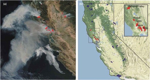
Figure 1. (a) Visible satellite imagery from the VIIRS instrument aboard Suomi-NPP and fire hot spot detections (red) from the VIIRS instrument aboard the Suomi-NPP satellite for October 9, 2017. The image is downloaded from NASA Worldview website. (b) Fire perimeters of the Atlas, Tubbs, Nuns, Redwood Valley, and Pocket wildfires (red). Other prescribed fires and wildfires occurring during the Oct 8–20, 2017 time period are shown in blue. Fire perimeters are from the GEOMAC system and hot spot locations are from the MODIS and VIIRS instruments aboard the Terra, Aqua and SUOMI-NPP satellites

California wildfires have been increasing in recent years for a combination of reasons, such as a warming climate, historical fire suppression policies, and a variety of pressures that put barriers on fuel treatments (Miller, Field, and Mach 2020). This trend is expected to continue, where California wildfires are estimated to increase in frequency and health impacts on a growing population due to the effects of climate change and global warming (Abatzoglou and Williams 2016; Flannigan et al. 2013; Spracklen et al. 2009). Under a medium-high temperature scenario, California wildfire emissions by the end of 2100 are projected to increase around 20–100% compared with the emissions in 1961–1990 (Hurteau et al. 2014). This projection also predicted the maximum increase of emissions in northern California. According to global climate model simulations of complex climate-fire-ecosystem interactions, the magnitude of increases in wildfire aerosol emissions is estimated to be as great as the corresponding reductions in emissions projected to result from air pollution control policies (Zou et al. 2020). This is already happening; McClure and Jaffe (2018) showed that, although most regions of the country have declining PM_2.5, the annual 98th percentile of daily averages is increasing in many parts of the western US, where wildland fires are increasing (Jaffe et al. 2020).

Emissions of PM_2.5 from wildfires in California have raised a series of concerns about their health impacts. Studies have analyzed the spatiotemporal correlations between wildfire PM_2.5 emissions and respiratory health effects, such as risk of asthma exacerbation and chronic obstructive pulmonary disease (Rappold et al. 2017, 2011; Reid et al. 2016a, 2016b). Other studies have evaluated the effects of wildfire smoke exposure on increased cardiovascular and cerebrovascular emergency department visits (Wettstein et al. 2018), acute myocardial infarction (Weichenthal et al. 2017), risk of hospital admissions (Gan et al. 2017; Liu et al. 2017), asthma-related outcomes (Borchers Arriagada et al. 2019; Lipner et al. 2019), and out-of-hospital cardiac arrests (Haikerwal et al. 2015; Hoshiko et al. 2019). The acute effect of fire smoke on children has been studied for symptoms such as increased eye and respiratory symptoms, medication use, and physician visits (Künzli et al. 2006). The economic cost of adverse health effects from wildfire emission exposure has been quantified (Fann et al. 2018; Kochi et al. 2010; Richardson, Champ, and Loomis 2012), and those studies pointed out the necessity of considering the monetary value of preventing these specific adverse health outcomes when forming wildfire management policy. In a study of the 2003 Canadian wildfires, Henderson et al. (2011) compared three measures of forest fire smoke exposure – air quality monitors, a dispersion model, and plumes in satellite images – and examined the resulting impacts of smoke on respiratory and cardiovascular health outcomes. Jaffe et al. (2020) provide a comprehensive critical review of wildfire and prescribed burning impacts on health and air quality in the United States.

A major challenge in studying the relationships between air pollution, weather or climate, and human health outcomes is how to characterize exposures at the population or individual level. There is a long history of improving estimates of particulate matter and other trace gas species in air quality modeling with methods such as bias correction, ensemble modeling, and Kalman filtering (e.g. Crooks and Özkaynak 2014; Djalalova, Monache, and Wilczak 2015; Huang et al. 2017; Zhang et al. 2020). Additionally, data fusion and machine learning techniques combine chemical transport model outputs, meteorological model outputs, remotely-sensed data, and surface monitoring data to improve air quality estimates (e.g. Al-Hamdan et al. 2014, 2009; Chu et al. 2016; Engel-Cox, Hoff, and Haymet 2004; Gupta and Christopher 2009; Liu et al. 2004; Van Donkelaar et al. 2010). Recent studies applied these methods to periods of wildland fire air quality impacts. These impacts are episodic in nature and can result in particulate matter concentrations well above mean values, conditions that can confound the performance of otherwise successful bias correction approaches (e.g. Huang et al. 2017). Some of the first works combining surface measurements, remotely-sensed data, and modeled data for wildland fire smoke exposure were in British Columbia, Canada, using empirical models to estimate daily PM_2.5 concentrations (Yao and Henderson 2014; Yuchi et al. 2016). Lassman et al. (2017) used a ridge-regression model to estimate PM_2.5 exposure from smoke during the 2012 Washington wildfires; this method was adopted by Gan et al. (2020) and applied to the 2013 Oregon wildfires. Other geostatistical studies combined chemical transport model outputs, meteorological model outputs, satellite observations, and surface monitoring data. Zou et al. (2019) used three machine learning algorithms to estimate PM_2.5 exposure from the 2017 wildfires in the Pacific Northwest; Cleland et al. (2020) used the Constant Air Quality Model Performance and Bayesian Maximum Entropy methods for the 2017 Northern California wildfires; Bi et al. (2020) used AOD and purple air monitoring data in a random forest model for the 2018 California wildfires; O’Dell et al. (2019) used two methods for the continental US; and Geng et al. (2018) used a Bayesian ensemble model for Colorado wildfires in 2011–2014.

In a comprehensive review, Diao et al. (2019) examined the methods, data sources, and applications of surface PM_2.5 estimates from eleven datasets of daily and annual PM_2.5 concentrations for the continental U.S. that were derived using a mix of surface monitoring data, chemical transport modeling, and remotely sensed data. They found that several of these publicly available, frequently used PM_2.5 datasets showed significant discrepancies with each other at county-average level in the contiguous United States. This study highlighted the importance of conducting inter-comparison studies on PM_2.5 estimates and contrasting the methods used for deriving them. Therefore, we simulated air quality conditions using a suite of remotely sensed data, surface observational data, chemical transport modeling, and data fusion and machine learning methods to arrive at datasets useful to air quality and health impact analyses specific to wildland fire.

We focused on the five large wildfires comprising the Wine Country wildfires of October 8–20, 2017 that occurred in Napa and Sonoma Counties of California, known for their extensive vineyards and wineries. These were the Atlas (52 K acres), Tubbs (37 K acres), Nuns (57 K acres), Pocket (17 K acres), and Redwood Valley Incident (37 K acres) wildfires. Figure 1 shows the fire perimeters in red. Mass and Ovens (2019) gave a detailed analysis of the meteorological conditions preceding and during the wildfire period. Strong offshore winds downed power lines the evening of October 8, igniting the Tubbs fire at about 2145 PDT. Wind gusts ranged from 30 to 50 m/s, rapidly spreading the fires; for example, the Tubbs wildfire traveled over 19 km in the first 3 hours (Griggs et al. 2017). These strong, dry, offshore “Diablo” winds are similar to Santa Ana winds that occur in southern California; they usually occur in the fall and winter and are generally strongest at night (Smith, Hatchett, and Kaplan 2018).

In Sonoma County, coniferous forest and oak woodlands comprise about 50% of the land area, with some redwood ecosystems and coastal prairie grasses. Historically, frequent low-intensity fires were part of the natural ecology of many of these ecosystems, consuming dead vegetation and small trees, leaving more large trees alive. Growth of the wildland urban interface (WUI), where one-third of the Sonoma population live, along with land ownership fragmentation and effective fire suppression, have led to a buildup of vegetation on the landscape (Sonoma County, 0000). Before ignition on October 8, conditions were typically although not abnormally dry (Mass and Ovens 2019), but substantial precipitation in the previous winter had enhanced the growth of fine fuels such as grasses and shrubs, providing a plentiful fuel source for a potential ignition (Dudney et al. 2017). Such an ignition occurred when high winds downed trees and powerlines (Keeling 2018), igniting the plentiful dry fuels. Historically, many coastal-proximal ecosystems in California are “ignition-limited”, meaning that non-human sources of ignition (e.g. lightning) are rare during periods when fuels and climate are suitable for burning; interior forests and deserts experience frequent lightning strikes (Steel, Safford, and Viers 2015). Today, ignitions based on equipment use, smoking, campfire, railroad, arson, debris burning, fireworks, and powerlines account for 84% of wildfires and 44% of the area burned nationally (Balch et al. 2017), causing ignitions in previously ignition-limited ecosystems.

In this study, we conducted air quality modeling, data fusion, and machine learning analyses of wildland fire smoke impacts for October 8–20, 2017, to characterize population-level smoke exposure. We generated two fire emissions inventories and used them in two air quality modeling system simulations along with an anthropogenic emission inventory customized for Northern California. A third air quality simulation was run without fires. Data fusion and three machine learning approaches were then applied to optimize datasets for smoke exposure estimates. The net result was seven datasets (3 predictions, 4 analyses) of daily PM_2.5 concentration estimates appropriate for use in an exposure-response relationship to estimate the mortality attributable to the wildfire smoke. Section 2 details the data and methods used. In Section 3; we discuss fire emissions calculations; evaluate three air quality modeling simulations, a data fusion method, and three machine learning methods; and use the optimally performing dataset to estimate regional health effects of the wildfire smoke. Challenges and perspectives for future studies are discussed in Section 4.

Data and methods

During October 8–20, 2017, ground-based and remotely sensed data were brought together for regional modeling of near-surface PM_2.5 concentrations, and one data fusion and three machine learning methods were applied to optimize datasets for smoke exposure estimates over California from five major wildfires: Nuns, Pocket, Redwood Valley, Tubbs and Atlas (Figure 1). First, a fire emission inventory was developed using GOES-16 Advanced Baseline Imaging (ABI), Visible Infrared Imaging Radiometer Suite (VIIRS) and Moderate Resolution Imaging Spectroradiometer (MODIS) fire detections and Fire Radiative Power (FRP). These data were used in two air quality modeling system simulations along with an anthropogenic emission inventory customized for Northern California. A third air quality simulation was run without fires. Data fusion and three machine learning approaches were then applied. The net result was seven datasets (3 predictions, 4 analyses) of daily PM_2.5 concentration estimates appropriate for use in an exposure-response relationship to estimate the mortality attributable to the wildfire smoke.

Surface monitoring data

Ground-based observational data were obtained for October 2017 from two sources: The first source was the US Environmental Protection Agency (EPA) Air Quality System (AQS, https://www.epa.gov/aqs), which contains ambient air pollution data collected by EPA, state, local, and tribal air pollution control agencies from thousands of monitors. The second source was from the cache of temporary monitors deployed during wildfire operations by the Interagency Wildland Fire Air Quality Response Program (IWFAQRP) and the California Air Resources Board (CARB). In California, these monitors are Environmental Beta Attenuation Monitors (EBAM; Met One Instruments, Inc.). Laboratory (Trent 2006) and field (Schweizer, Cisneros, and Shaw 2016) studies evaluating EBAM performance with federal reference method monitors (which comprise most of the permanent monitoring network) found correlations greater than 0.9 with a tendency of the EBAM to overestimate PM_2.5 especially when relative humidity was greater than 40% (Schweizer, Cisneros, and Shaw 2016). Data were accessed and processed by the PWFSLSmoke R statistical package developed by Mazama Science (https://github.com/MazamaScience/PWFSLSmoke).

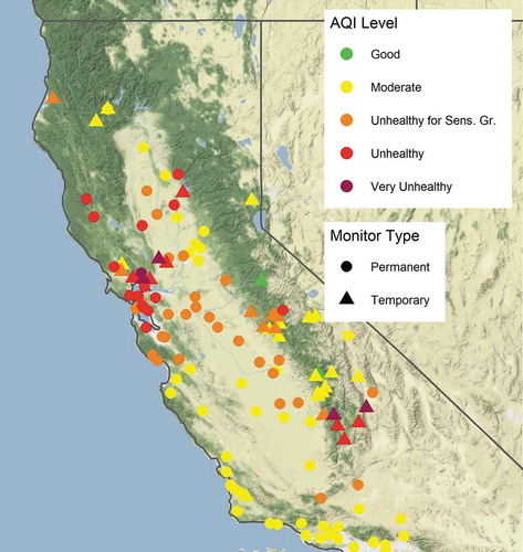
Figure 2 shows the locations of the permanent and temporary PM_2.5 monitors. The locations are color-coded by the maximum EPA Air Quality Index (AQI; https://www.airnow.gov/aqi/aqi-basics/) measured during October 6–20, 2017. AQI translates 24-hr average PM_2.5. concentrations into actionable health information: Good (green), Moderate (yellow), Unhealthy for Sensitive Groups (USG, orange), Unhealthy (red), Very Unhealthy (brown), and Hazardous (purple). Many locations across California had USG and Unhealthy conditions, and several days in Napa and the southern Sierra Nevada Mountains had Very Unhealthy conditions. The maximum 24-hr average PM_2.5 concentration in the southern Sierras (204 μg/m³) was measured at a temporary monitor. The maximum 24-hr average PM_2.5 concentration in Northern California (193 μg/m³) was measured at a permanent monitor in Napa.

Figure 2. Locations of PM_2.5 air quality monitors. Circles are permanent monitors from the EPA AQS System. Triangles are temporary monitors deployed for wildfires. The circles and triangles are color-coded by the Air Quality Index by the maximum measured 24-hr average PM_2.5 value during the October 6–20, 2017 time period

MODIS Aerosol Optical Depth (AOD)

The MODIS Multi-Angle Implementation of Atmospheric Correction (MAIAC) retrieval algorithm accomplishes atmospheric correction via a relatively new method that is encoded in a generic algorithm designed to work with MODIS data to facilitate deriving both aerosol and land surface reflectance products (Lyapustin et al. 2011a, 2011b, 2012, 2018; NASA 2020a). Based on a time series of MODIS measurements and spatial analysis, this algorithm simultaneously retrieves atmospheric aerosols and bidirectional reflectance from MODIS data (NASA 2020a). It further detects clouds and corrects atmospheric effects over both dark (vegetated) surfaces and bright (desert) targets. MAIAC provides a suite of atmospheric and surface products in HDF4 format, including (1) daily MCD19A1 (spectral BRF, or surface reflectance), (2) daily MCD19A2 (atmospheric properties), and (3) 8-day MCD19A3 (spectral BRDF/albedo). The MAIAC Daily Atmospheric Properties Product (MCD19A2) over land includes the following properties at a 1-km spatial resolution: column water vapor (CWV), cloud mask, aerosol optical depth (AOD), aerosol type (background/smoke/dust), and smoke injection height (Lyapustin and Wang 2018; NASA 2020b). For this study, we processed daily MAIAC AOD for the month of October 2017 for use in the machine learning products and used the standard MODIS AOD in the data fusion product.

Fire emission inventories and Chemical Transport Modeling (CMAQ)

We conducted regional air quality modeling using the Community Multiscale Air Quality (CMAQ) modeling system v5.2 (Appel et al. 2017) with meteorology from the Weather Research and Forecasting (WRF) model version 3.7 (Skamarock et al. 2008). Three WRF-CMAQ simulations were conducted, as summarized in Table 1 and discussed here; one without fires and two with fires. The anthropogenic emission inventory used California Air Resources Board’s (CARB) emission inventory for area and nonroad sources, EMFAC2017 model output for on-road sources, and the Bay Area Air Quality Management District (BAAQMD) facility-level emissions data for point sources. Biogenic emissions were from the EPA BEIS3.61. Fire activity data were collected from the GOES-16 ABI instrument, the Terra and Aqua MODIS instrument, and the SUOMI-NPP VIIRS instrument. Fire emissions were calculated using the BlueSky Smoke Modeling framework (BSF; Larkin et al. 2009). The total modeling time period was October 2–20, 2017. The first several days were discarded as model spin-up, providing an analysis time period of October 6–20, 2017.

Table 1. WRF-CMAQ model simulation summary

Settings	No Fires	Baseline	GTP
Period	Oct 2–20, 2017	Oct 2–20, 2017	Oct 2–20, 2017
Resolution	Horizontal: 4-km Vertical: 37 layers	Horizontal: 4-km Vertical: 37 layers	Horizontal: 4-km Vertical: 37 layers
Meteorology	WRF v3.7	WRF v3.7	WRF v3.7
Chemistry	CMAQv5.2, SAPRC07, AERO6	CMAQv5.2, SAPRC07, AERO6	CMAQv5.2, SAPRC07, AERO6
Fire Emissions	–	BlueSky v3.5.1	BlueSky v3.5.1
Fire Activity	–	Five Wine Country Fires: GOES-16 Other Fires: MODIS/VIIRS	Five Wine Country Fires: GOES-16 Other Fires: MODIS/VIIRS
Fire Diurnal Profile	–	Five Wine Country Fires: CMAQ (default) Other Fires: CMAQ (default)	Five Wine Country Fires: GOES-16 Other Fires: CMAQ (default)
Non-Fire Emissions	CARB area and non-road, EMFAC2017 on-road, BAAQMD facility-level point source emissions, BEIS3.61	CARB area and non-road, EMFAC2017 on-road, BAAQMD facility-level point source emissions, BEIS3.61	CARB area and non-road, EMFAC2017 on-road, BAAQMD facility-level point source emissions, BEIS3.61

Fire activity for the five large wildfires comprising the Napa Wine Country fires was based on the GOES-16 satellite fire detections. The GOES-16 satellite was launched November 2016 and became operational in December 2017. It views the earth from the equator at a location southeast of Florida. Previous GOES suites had 5 spectral bands, returning data every 15 minutes at a 4-km resolution at nadir. The GOES-16 ABI (Schmit et al. 2017, 2018) instrument has 16 spectral bands, returning data every 5 minutes at a 2-km resolution at nadir. This dramatically improves the ability to view fire progression in real time and translates to an improvement in our capability to model hourly smoke production, making it possible to calculate fire emissions in near-real time as the fire moves from pixel to pixel. For those pixels with the highest-quality retrieval, the GOES Fire Detection and Characterization (FDC) product provides an estimate of FRP, which is an observation of instantaneous energy release. However, many pixels that identified burning did not have enough information to estimate FRP, for example because the satellite view is obscured by thick smoke. For each pixel location, we interpolated temporally between those instances where FRP was estimated to create a complete FRP record for each location at 5-minute resolution. Then we integrated the 5-minute data to produce hourly total Fire Radiative Energy (FRE) at each pixel. This fire activity information was used in the two modeled fire cases for the five large wildfires.

Total emissions per day per fire pixel location were calculated using the BlueSky smoke modeling framework (BSF; Larkin et al. 2009). BSF has long been used operationally in the US Forest Service smoke forecasting products (Larkin et al. 2009; Strand et al. 2012), the EPA National Emission Inventory (Larkin et al. 2020), the Canadian BlueSky system (Schigas and Stull 2018; Yao, Brauer, and Henderson 2013), and AIRPACT-5 (Chen et al. 2008). Using BSF and the GOES-16 fire activity data, we created two wildfire modeling cases, Baseline and GOES Temporal Profile (GTP; see Table 1). For the GTP case, we used the hourly derived FRE to allocate the daily emissions to an hourly emissions profile. For the Baseline case, we used emissions calculated from the BSF allocated diurnally to the default diurnal profile in CMAQ (Appel et al. 2017), which is approximately gaussian in shape and maximum emissions occur at 1700 local time. Plume rise was calculated using the CMAQ plume rise (Pouliot et al. 2005) in the Baseline case and using the Briggs (1975) algorithm as implemented in BlueSky (Larkin et al. 2009) in the GTP case. In both cases the daily fire heat flux was allocated hourly according to the simulation time profile (e.g. Baseline or GTP), yielding hourly estimates of plume rise.

The Wine Country wildfires ignited late in the evening of October 8, and the GTP case allows us to capture this initial fire activity, with the first fire detection at approximately 22:00 PDT; behavior not captured in the default time profile of the Baseline case. Further, Li et al. (2019) analyzed FRP data from polar orbiting and geostationary satellites, deriving time profiles of emissions for over 40 US ecosystems, and discuss how forested ecosystems in the western US and in particular California exhibit nighttime fire activity. Thus, we were motivated to take advantage of the new GOES-16 fire detection data to simulate this fire behavior which led to widespread smoke impacts across the state in the morning of October 9.

Fire activity for the smaller fires in the modeling domain was based on the fire detections with higher spatial resolution, MODIS and VIIRS, provided in the NOAA Hazard Mapping System (HMS) product, as follows. First, for a given day, all HMS fire pixels were given a square buffer of a specified size, where the size of each square varied by satellite source. Sizes were determined roughly by the resolution size of the original satellite (e.g. VIIRS was 375 m and all other satellites were 1 km). Second, all intersecting squares were dissolved together into a set of disjoint polygons. Third, we summed the number of fire pixels within each polygon. Often when working with daily temporal resolution, satellites identify the same location multiple times over the course of the day. Because of this, we developed a reduced fire pixel counting method that grouped fire pixels together within 1 km. This was done by overlaying a 1-km resolution grid over each polygon, then summing the number of 1-km grid cells that contained at least one fire pixel. Lastly, area was then assigned to each polygon by multiplying the reduced number of fire pixels by an estimated size per pixel based on vegetation type (Larkin et al. 2020). Each polygon was now considered one fire location with a corresponding geographic location (center coordinates) and area estimation.

Data fusion

A major challenge in studying the relationship between air pollution, weather or climate, and human health outcomes is how to characterize population-level or individual-level exposures. Air quality modeling offers detailed information in time and space about potential exposure, but estimates are subject to high variability and uncertainties especially when modeling wildland fires (Baker et al. 2016; Jaffe and Widger 2012; Wilkins et al. 2018). Surface observations are sparse, but they offer the means to evaluate and constrain surface model output where available. Remotely sensed data are not sparse and offer a contiguous field of view, but they may be available only at snapshots during the day, such as from polar orbiting satellites, or give only an integrated view of the atmosphere, which may or may not reflect what is happening at the surface.

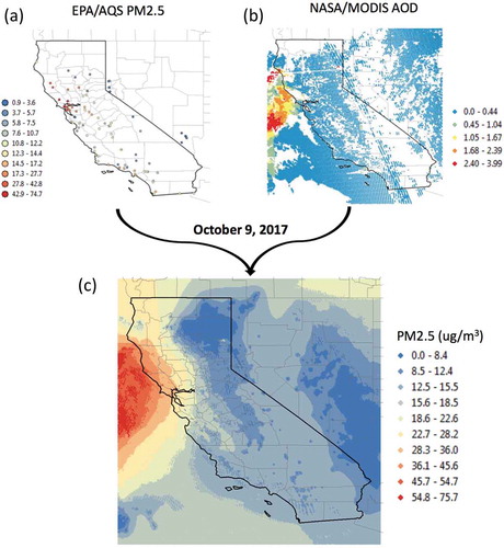
One promising method for characterizing environmental exposure for public health practice and epidemiologic research is the integration of remote sensing satellite systems data with monitoring network data (Al-Hamdan et al. 2014, 2009). Use of remotely sensed data can help to fill the temporal and spatial gaps found with ground-level monitor data. One PM_2.5 dataset in this study was created using a data fusion geostatistical surfacing algorithm of Al-Hamdan et al. (2009, 2014), which provided daily PM_2.5 on a 3-km grid for the entire state of California. This algorithm leverages data from the US EPA AQS and the NASA MODIS instrument on board the Aqua Earth-orbiting satellite (see Table 2). It estimates daily PM_2.5 concentrations using a regional spatial surfacing algorithm, which includes regression models, B-spline and Inverse Distance Weighted (IDW) smoothing models, a quality control procedure for the EPA AQS data, and a bias adjustment procedure for MODIS/Aerosol Optical Depth-derived PM_2.5 data (Al-Hamdan et al. 2014, 2009). The net result is daily estimates of PM_2.5 on a 3-km grid (surface) (e.g. Figure 3).

Table 2. Data fusion and machine learning approaches

Method	Modeling Dataset	Resolution	Surface Data	Meteorological Data	Remotely Sensed Data
Data Fusion (DF)	–	3-km	AQS	–	Standard MODIS AOD
Multi-linear Regression (MLR)	WRF-CMAQ-Baseline	4-km	AirNow	WRF, NARR	MAIAC AOD
Generalized Boosting (GB)	WRF-CMAQ-Baseline	4-km	AirNow	WRF, NARR	MAIAC AOD
Random Forest (RF)	WRF-CMAQ-Baseline	4-km	AirNow	WRF, NARR	MAIAC AOD

Figure 3. Illustration of the components involved in data fusion. (a) Surface PM_2.5 monitoring data from EPA AQS and (b) MODIS AOD merged to create (c) a surface of PM_2.5 concentrations on a 3-km grid for October 9, 2017

Previous work of Al-Hamdan et al. (2009, 2014), were applied to longer term studies such as a 2003–2008 PM_2.5 data fusion analysis which was linked with public health data from the REasons for Geographic And Racial Differences in Stroke (REGARDS) national cohort study and disseminated to users through the Centers for Disease Control and Prevention (CDC) Wide-ranging Online Data for Epidemiologic Research (WONDER) system. The CDC WONDER system is one of 10 systems providing publicly available PM_2.5 exposure datasets designed to support health risk assessment and epidemiological studies (Diao et al. 2019). The ready availability of the data inputs, robustness of the approach, and demonstrated utility for health analyses motivated us to include this methodology in this work.

Machine learning

Three machine learning-based algorithms were applied: an ordinary multi-linear regression (MLR) method, a generalized boosting (GB) method, and a random forest (RF) method. These methods incorporate the Baseline WRF-CMAQ modeling results with the AQS and MAIAC AOD, and meteorological variables, to produce improved 24-hr average near-surface PM_2.5 concentration estimates (see Table 2). Methodology as applied by Zou et al. (2019) for the 2017 Pacific Northwest wildfire season was used and is briefly summarized here. Previously, Reid et al. (2015) compared a set of 11 machine learning algorithms and demonstrated the favorable performance of the GB and RF methods for predicting PM_2.5 concentrations during a 2008 fire event in California. Few studies have used these novel methods for episodic wildland fire events, so the success of the Reid et al. (2015) and Zou et al. (2019) motivated their use here.

A two-step approach (Zou et al. 2019) was followed, where the first step was to gap-fill for spatiotemporal missing values in the MAIAC satellite AOD retrievals. This was based on (1) three hourly meteorological variables: total cloud fraction, cloud liquid water content, and surface water vapor mixing ratio from the WRF outputs; (2) two geographical variables: terrain elevation and vegetation coverage; and (3) the simulated hourly AOD from the WRF-CMAQ Baseline case. The second step involved data fusion for optimizing daily surface PM_2.5 concentrations from the WRF-CMAQ Baseline case, based on (1) daily averages of observational AirNow surface PM_2.5 measurements; (2) gap-filled AOD from Step 1; and (3) six meteorological variables: surface wind speed and directions at 10 m, surface air temperature at 2 m, relative humidity at 2 m, precipitation rates at surface on a log scale, and planetary boundary layer heights from the North American Regional Reanalysis (NARR) data (NCEP 2005) produced by the National Centers for Environmental Prediction.

Quantitative analysis

Five quantitative analysis metrics were used to evaluate model performance (Table 3). Mean bias indicates how a modeled (M) solution tends to over- or underestimate compared to observational (O) data. The mean bias can be skewed or overly influenced by outlier/high-value data; therefore, the median absolute difference and fractional bias are used to reduce this influence. Pearson correlation (r) measures the linear correlation between the modeled and observed data pairs (1: perfect positive correlation, −1: perfect negative correlation, 0: no correlation). Root Mean Square Error (RMSE) is the standard deviation of the residuals, where residuals are a measure of how far data points are from the regression line, and is an indication of how concentrated the data are around the line of best fit.

Table 3. Definitions of quantitative analysis metrics. M = modeled data. O = observed data

Metric	Equation
Mean Bias	$\frac{1}{n}\sum _1^n\left(M-O\right)$
Median Absolute Difference	$Median\left(\left|M_i-O_i\right|,i=1,n\right)$
Fractional Bias	$\frac{1}{n}\left(\frac{\sum _1^n\left(M-O\right)}{\sum _1^n\left(\frac{\left(M+O\right)}{2}\right)}\right)$
Pearson Correlation (r)	$\frac{{\sum }^{\left(M-\bar{M}\right)}\left(O-\bar{O}\right)}{\sqrt{{\sum }^{{\left(M-\bar{M}\right)}^2}{\sum }^{{\left(O-\bar{O}\right)}^2}}}$
Root Mean Square Error (RMSE)	$\sqrt{\frac{\sum _1^n{\left(M-O\right)}^2}{n}}$

Health outcome exposure-response function

We assessed regional health impacts from the 2017 Wine Country wildfire smoke using a relative risk function for multiple-cause mortality due to PM_2.5 exposure, following the method of a smoke impact health assessment study by Johnston et al. (2012) as applied by Zou et al. (2019). Using the following exposure-response function, we calculated the multiple-cause mortality attributable to PM_2.5 exposure during the fire smoke pollution episode:

$\mathrm{M}\mathrm{o}\mathrm{r}\mathrm{t}\mathrm{r}\mathrm{a}\mathrm{l}\mathrm{i}\mathrm{t}\mathrm{y}\mathrm{a}\mathrm{t}\mathrm{t}\mathrm{r}\mathrm{i}\mathrm{b}\mathrm{u}\mathrm{t}\mathrm{a}\mathrm{b}\mathrm{l}\mathrm{e}\mathrm{t}\mathrm{o}\mathrm{P}{\mathrm{M}}_{2.5}\mathrm{e}\mathrm{x}\mathrm{p}\mathrm{o}\mathrm{s}\mathrm{u}\mathrm{r}\mathrm{e}=\sum _{P{M}_{2.5}}^n{D}_{PM2.5}\times M\times (R{R}_{SI}(P{M}_{2.5})-1)$

where PM_2.5is daily average surface PM_2.5 concentrations (minimum value: 5 μg/m³, maximum value: 200 μg/m³). Following Johnston et al. (2012), we excluded the grid cells with daily exposure estimates of less than 5 μg/m³ and fixed grid cells with exposure estimates larger than 200 μg/m³ to a maximum threshold of 200 μg/m³. D_PM2.5 is the number of days with daily PM_2.5 at certain levels between each PM_2.5 concentration interval (i.e. each 1-μg/m³ increment between 5 μg/m³ and 200 μg/m³), n is the total number of concentration intervals, and M is the county-level daily average number of multiple cause of deaths between October and December 2017. RR_SI is a relative risk function for multiple-cause mortality due to short-term PM_2.5 exposure; in this study, we applied a relative risk of 1.1% (95% CI: 0, 0.26%) per 10 μg/m³ increase of surface PM_2.5 concentration as estimated by Johnston et al. (2012) based on three studies of wildfire smoke, including Hänninen et al. (2009). This relative risk is consistent with the range of estimates of short-term mortality related to urban PM_2.5 exposure (Pope and Dockery 2006).

We obtained all-cause mortality data from the Centers for Disease Control (CDC) Wide-ranging Online Data for Epidemiologic Research (WONDER) online database and demographic data from the 2010 USA Census Grids provided by the NASA Socioeconomic Data and Applications Center (SEDAC). We downscaled the county-level multiple cause of deaths (M) to the model-grid scale according to the high-resolution gridded population density data from the 2010 USA Census Grids. Therefore, we were able to estimate population exposure risks with both gridded mortality and PM_2.5 concentrations at the same resolution of the modeling grids (i.e. 3 km, 4 km).

Results and discussion

Fire emissions

The Wine Country wildfires of October 8–19, 2017 ignited late in the evening of October 8. They quickly became devastating to human life and property and caused widespread smoke impacts to millions of people. To capture this initial fire activity, we relied on the GOES-16 FDC products which identified the first detection at approximately 22:00 PDT. Using these data, we estimated emissions hourly to capture the widespread smoke impacts as seen by the MODIS instrument at approximately 11:30 PDT on October 9 (Figure 1). The hourly FRE was aggregated across the fire to produce the time profile of emissions (Figure 4, dashed line). This method has also been used to simulate the early-morning explosive Camp wildfire (O’Neill and Raffuse 2021). Others have discussed the sensitivity of modeled concentrations to the temporal distribution of fire emissions (e.g. Garcia-Menendez, Hu, and Odman 2014; Larkin et al. 2012; Wilkins et al. 2018).

Figure 4. Hourly PM_2.5 emissions from wildfires and prescribed fires in California, October 8–20, 2017. Black line (Baseline): diurnal profile of the emissions from the five Wine Country wildfires, calculated using BSF and allocated hourly based on the default profile in CMAQ. Dashed line (GTP): hourly emissions from the five Wine Country wildfires, calculated using BSF and allocated hourly based on GOES-16 FDC data. Gray line (Other Fires): hourly emissions from all other fires, calculated using BSF and allocated hourly based on the default profile in CMAQ

Figure 4 highlights the differences between the default (Baseline) and GOES-16 (GTP) temporal emissions profiles for the five Wine Country wildfires. The default profile misses the significant activity that occurred late in the evening of October 8 and early morning of October 9, delaying emissions for several hours. These differences in emission timing propagate through the initial 12–24 hours in the smoke transport modeling, but thereafter the Baseline and GTP results are similar. Later in the modeling period (October 16–19), the peak of the GTP profile often shifted into the evening hours. Similar behavior was found by Li et al. (2019), who noted that with these wind-driven fires, especially in California, evening and nighttime fire activity is apparent in the satellite fire activity data.

The fires burned through about 10 fuel types ranging from grasslands and shrublands to heavily forested systems. The fuel type has a large effect on the quantity of emissions estimated and can be responsible for wide variability in emissions (Drury et al. 2014; Prichard et al. 2019). Fuel heterogeneity and variability also mean that acres burned are not necessarily a good proxy for emissions. In the case of the Wine Country wildfires, 10% of the total burned area was responsible for 62% of the PM_2.5 emissions, because it was in heavily forested vegetation. In contrast, shrublands comprised 38% of the total acreage burned but caused only about 15% of the total emissions.

Other fire activity occurred throughout the modeling domain, such as crop residue burning in the Sacramento and San Joaquin Valleys, prescribed burning operations in the Sierra Nevada Mountains, and several small wildfires (Figure 1b, blue dots; Figure 4, gray line shows estimated hourly emissions). The estimated emissions from the five Wine Country wildfires totaled 49 K tons, exceeding the total emissions of 43 K tons from all other fires in the state for the modeled time period.

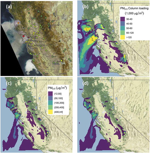
Figure 5 shows smoke transport at 11:00 am PDT as viewed by the GOES-16 satellite and modeled by the Baseline and GTP cases. The Baseline and GTP cases are very similar except for the Redwood Valley fire (the northernmost of the five wildfires), where GTP had greater PM_2.5 concentrations at the surface than did Baseline. Figure 5 also illustrates how surface and upper-level transport patterns can differ. The satellite views the top of the atmosphere, so we provide a modeled column-integrated PM_2.5 estimation to compare with the satellite. Overall, the transport patterns line up with many of the visible satellite imagery characteristics, with smoke reaching across the Pacific in a more directly eastward direction than the more south-flowing surface plume.

Figure 5. Panel of visible satellite imagery and WRF-CMAQ runs at 11:00 am PDT October 9, 2017. (a) Visible GOES-16 satellite imagery and surface 24-hr average PM_2.5 concentrations (circles) from EPA AirNowTech color-coded by air quality index (Figure: NOAA AerosolWatch) (b) the Baseline total column PM_2.5, (c) the Baseline surface 1-hr average PM_2.5 concentration, and (d) the GTP surface 1-hr average PM_2.5 concentrations (same scale of PM_2.5 concentrations as in 5c)

WRF-CMAQ model simulations

We used observed PM_2.5 concentration data measured at the permanent and temporary monitoring locations to evaluate the spatial distributions of concentrations from the WRF-CMAQ model simulations. We grouped monitor locations into eight regions (Figure 6a) to account for the coastal, central valley and mountainous regions of the State. The coastal and coast range monitors were grouped, north to south, into the Northern, Wine Country, Bay Area, Central Coast, and Southern California regions. Inland monitors were grouped into the Sacramento Valley, San Joaquin Valley, and Sierra regions. To give a temporal profile of model performance, the 24-hr average PM_2.5 concentrations were averaged together by region each day, both for observations and for each of the seven model and analysis datasets (Figure 6b).

Figure 6. (a) Locations of PM_2.5 monitors grouped by region. (b) Time series comparison of measured and modeled 24-hr average PM_2.5 concentrations by region. Black lines: observations; colored lines: WRF-CMAQ model simulations (NoFires, Baseline, and GTP), data fusion (DF), and three machine-learning analyses (GB, MLR, and RF). See key at top

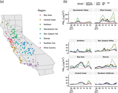
The WRF-CMAQ Baseline and GTP model simulations performed well during the beginning and middle of the modeling period (October 8–15) and tended to overestimate PM_2.5 concentrations on October 15–17. This overestimation is most apparent at the locations close to the fires (Wine Country, Bay Area). The later-period overestimation was also apparent in the regions through the interior of the state (Sacramento Valley, San Joaquin Valley, Sierras) where the other fires were active. On October 10, the WRF-CMAQ simulation results were much higher (by more than a factor of two) at monitoring locations in the Sacramento Valley. This was due not only to smoke from the Wine Country fires but also to fires that had started on October 9 in the Sierra foothills (Figure 1, fire perimeters in blue) and fires in the Sacramento Valley. These fires initially deposited smoke into the Valley, then afternoon west winds brought smoke from the Wine Country to the Valley.

Evaluation of the WRF-CMAQ Baseline and GTP model simulations at the permanent and temporary monitoring locations shows more similarities than differences. Pearson correlation and RMSE were virtually the same at the permanent monitoring locations (approximately 0.65 and 12 µg/m3, respectively) and similar at the temporary monitoring locations (less than a 0.05 and 1 µg/m3 difference respectively). Baseline performed a bit better with a mean bias of 4 µg/m3 compared to 9.31 µg/m3 (Tables 4, 5). Overall, both runs were biased high; similar with other CMAQ simulations for fires (e.g., Wilkins et al. 2018; Zhou et al. 2018). Although timing of emissions made a difference in the PM_2.5 concentrations modeled in the Wine Country region, using the more detailed GOES-16 -based temporal profile did not necessarily improve the modeling results from the Baseline diurnal profile. Other work of O’Neill and Raffuse (2021) and Larkin et al. (2012) show that timing of emissions can be important to model performance such as at the fire start or when the boundary layer is low.

Table 4. Permanent monitor location analysis. Numbers in bold and italics are the best and second-best model performer respectively. 1179 data points (mean and standard deviation) or data pairs (other metrics) for all cases except in the DF case, where there are 1327 data points/pairs

Model	Mean (µg/m^3)	Standard Deviation (µg/m^3)	Pearson Correlation	RMSE (µg/m^3)	Fractional Bias	Mean Bias (µg/m^3)	Median Absolute Difference (µg/m^3)
NoFires	11.33	6.37	0.03	16.20	−0.23	6.71	5.76
Baseline	24.95	25.71	0.65	12.25	0.16	6.91	6.08
GTP	26.64	38.19	0.64	12.65	0.19	8.60	5.82
DF	16.81	15.26	0.95	5.73	−0.04	−1.23	0.71
GB	17.25	12.25	0.81	9.60	−0.02	−0.79	3.45
MLR	16.66	11.19	0.68	11.95	−0.04	−1.38	4.11
RF	17.63	11.84	0.86	8.32	−0.01	−0.41	2.66
Measured	18.04	15.48

Table 5. Temporary monitor location analysis. Numbers in bold and italics are the best and second-best model performer respectively. 406 data points (mean and standard deviation) or data pairs (other metrics) for all cases

Model	Mean (µg/m^3)	Standard Deviation (µg/m^3)	Pearson Correlation	RMSE (µg/m^3)	Fractional Bias	Mean Bias (µg/m^3)	Median Absolute Difference (µg/m^3)
NoFires	5.59	3.98	−0.05	24.87	−0.61	−17.16	9.85
Baseline	26.84	44.16	0.34	22.93	0.08	4.10	6.80
GTP	32.06	69.81	0.29	23.58	0.17	9.31	6.95
DF	11.98	7.00	0.38	23.23	−0.31	−10.76	4.96
GB	18.24	15.86	0.50	21.62	−0.11	−4.51	5.11
MLR	17.55	18.59	0.35	22.92	−0.13	−5.19	4.75
RF	18.49	15.55	0.49	21.74	−0.10	−4.25	4.85
Measured	22.75	24.84

Finally, Southern California was minimally impacted by these fires, and the NoFires case, while seemingly inconsequential, clearly shows how wildfire smoke can dominate as an emission source. This underestimation of emissions in the NoFires case illustrates the importance of properly accounting for wildfires as an emission source. The WRF-CMAQ mean bias ranged from −7 µg/m³ for the NoFires case to ~8 µg/m³ for the Baseline & GTP cases. This negative to positive switch of 15 µg/m³ was within the range of the ~25 µg/m³ value reported for a California wildfire by Wilkins et al. (2018). Here our overall model baseline bias was 0.65 which closely matched the 0.67 value in Wilkins et al. (2018) for a similar area. Fractional bias’s and correlations for the Baseline and GTP cases were both improved over results of Zou et al. (2019) and Herron-Thorpe et al. (2014).

Data fusion and machine learning

To solve the periodic high bias in the modeled PM_2.5 results, we applied the data fusion approach of Al-Hamdan et al. (2009, 2014) and the three machine-learning-based approaches of Zou et al. (2019). As expected, results were much improved, and these four methods compared well to measured PM_2.5 concentrations at the permanent monitoring data locations (Figure 7, Table 4). The DF and RF cases performed optimally across the metrics: DF had a Pearson correlation of 0.95, median absolute difference of 0.71 µg/m³, and RMSE of 6 µg/m³, and RF had the lowest bias metrics of −0.1 (fractional bias) and −4.25 µg/m³ (mean bias). This was much improved from the WRF-CMAQ Baseline and GTP modeled Pearson correlation scores of 0.64 and 0.65, RMSE of 12–13 µg/m³, and high bias tendency.

Figure 7. Comparison of measured (x-axis) and modeled (y-axis) 24-hr average PM_2.5 concentrations at all monitoring locations. Red circles: permanent monitors; blue circles: temporary monitors. The top panels are the three WRF-CMAQ modeling results and the four bottom panels are the data fusion (DF) and machine learning (MLR, GB, and RF) results

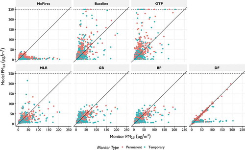
We also had the opportunity to independently evaluate these approaches at the temporary monitoring locations, which were not used in deriving the products. The temporary monitors were deployed specifically to measure air quality during wildfires and prescribed fire operations at locations that do not already have a permanent monitor. During the period of the Wine Country fires, most of the temporary monitors were located in the Sierras and Wine Country (Figure 2). The scatterplots in Figure 7 illustrate the high bias and departures from the 1:1 line seen in the modeling results at both the permanent (red) and temporary monitoring locations (blue). Figure 7 also shows how the high bias was improved upon in the data fusion and machine learning results, except in the MLR case, which has a higher scatter and RMSE of 12 µg/m³ at the permanent monitoring locations very similar to the WRF-CMAQ results.

All cases tended to perform better at the permanent monitor locations than at the temporary monitoring locations, which was expected with the data fusion and machine learning methods, which by definition incorporate these data, but less expected in the WRF-CMAQ runs. At the temporary monitor locations, Table 5 data show Pearson correlations ranged from 0.29 to 0.50 and RMSE ranged from 22 to 24 µg/m³ for the two WRF-CMAQ runs with fires and the data fusion and machine learning approaches. Median absolute difference data, which tend to be less sensitive to the data extremes (e.g. high PM_2.5 concentrations), ranged from 1–6 µg/m³ at the permanent locations and 5–10 µg/m³ at the temporary locations. The only exception to this trend was in terms of bias; the Baseline case performed better at the temporary monitor locations than at the permanent monitor locations. Many of these temporary monitor locations are in areas of complex terrain such as the Sierras, and the 4-km grid resolution is not necessarily a high enough resolution to resolve terrain features and smoke flows through them. Also, given that these temporary monitors dominated in the Sierras where there were few permanent monitors, the DF approach did not have a chance to calibrate to the area.

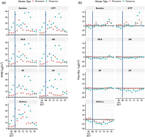
Figure 8 illustrates daily model performance, and we see how the overestimation bias in the WRF-CMAQ model simulations (Baseline, GTP) occurred in the later modeling period (October 16–18). Overall, the data fusion and machine learning results minimized bias well at both the temporary and permanent monitor locations. RMSE was consistently similar across all cases at the temporary monitor locations, while at the permanent monitor locations the DF case performed best. Of the data fusion and machine learning approaches, the RF case performed the most optimally across most metrics, with lowest or second-lowest RMSE, fractional bias, mean bias, and median absolute difference, and second-best Pearson correlations (0.86 and 0.49 at the permanent and temporary monitors, respectively). Zou et al. (2019) similarly found optimal performance with the RF case. Further, our machine learning results here were similar (in terms of fractional bias) and improved in terms of correlation and RMSE as compared to Zou et al. (2019). Cleland et al. (2020) in related work used Constant Air Quality Model Performance and Bayesian Maximum Entropy (BME) methods to estimate surface PM_2.5 concentrations for this same wildfire period with a correlation of 0.71. They incorporated the temporary monitoring data into their methods and note that adding temporary station data (in addition to the permanent monitors) to the BME estimation improves accuracy, with a 36% increase in correlation.

Figure 8. Daily model performance at the permanent (red) and temporary (blue) monitor locations in terms of (a) root mean square error (RMSE) and (b) mean bias. Vertical blue lines indicate October 8, 2017, the start of the wildfires

Air quality and health impact assessment

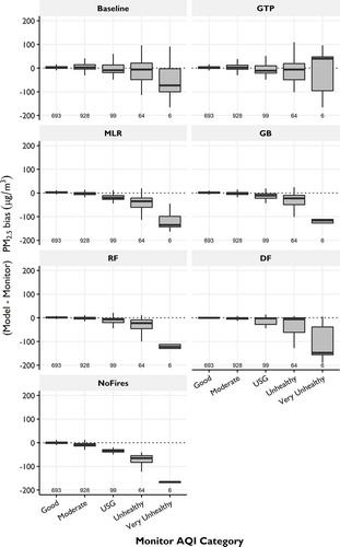
We used two approaches to investigate health impacts from these wildfires. The first approach compares surface 24-hr average PM_2.5 concentrations with the NAAQS and bins the data by AQI category. Figure 9 shows the modeled minus monitor bias for each of the seven datasets in this analysis by AQI category and the number of observations in each category. The data fusion and machine learning methods (DF, GB, MLR, RF) all tended to underestimate PM_2.5 concentrations in the Unhealthy/Very Unhealthy categories, and in general their data had much less variability than the WRF-CMAQ modeling approaches. For the highest health impact AQI categories, the two WRF-CMAQ simulations and the DF data fusion case had median Unhealthy bias near zero, while the other cases were biased less than zero. The GTP was the only case where the bias was not less than zero for the Very Unhealthy category. These biases can be important to smoke forecasters, because it is more important to not miss an event (such as an Unhealthy or worse air quality condition) than to forecast an event that does not materialize (Ainslie, So, and Chen 2020). Approximately 10% of the monitor-days measured exceedances of the NAAQS standard of 35 µg/m³. The Very Unhealthy data points were in Napa and the southern Sierras where the temporary monitors were located. These temporary monitors tend to be in small, rural communities, and compared to the permanent monitoring networks, the temporary sites typically have much higher concentrations of PM_2.5 and more days where PM_2.5 exceeds the NAAQS standard of 35 µg/m³ (Larkin 2019).

Figure 9. PM_2.5 bias by Air Quality Index (AQI) category. The numbers at the bottom of each panel are the number of model-monitor pairs in the AQI category

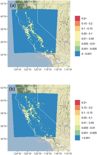
Finally, we used the approach of Zou et al. (2019), who applied the relative risk function for multiple-cause mortality due to PM_2.5 exposure of Johnston et al. (2012) to evaluate health impacts from these wildfires for October 8–20, 2017. Figure 10a shows the premature deaths related to PM_2.5 across the region (shown in blue) estimated from the NoFires WRF-CMAQ modeling case, and Figure 10b shows the additional mortality estimated from the RF case. Without the wildland fires, mortality due to PM_2.5 exposure was estimated as 44 deaths (95% confidence interval: 0, 105). Including the Wine Country wildfires and other smaller wildland fires increased the estimated mortality to 83 (95% confidence interval: 0, 196), almost doubling the number of deaths. This illustrates the profound effect that even a 12-day exposure to wildfire smoke can have on human health. It should be noted that a mortality of 83 is within the 95% confidence interval of the NoFires case and thus a possible outcome for that case as well. Spatially across the State (Figure 10), the additional mortality was in the highly populated Bay Area, Wine Country, and Sacramento Valley regions, where the highest smoke impacts were measured. Mortality also spread into more lightly populated areas of Northern California and the Tahoe-Reno-Carson area at the California/Nevada border; an area that had not showed mortality in the NoFires case. Mortality due to PM_2.5 exposure in the San Joaquin Valley was mostly attributable to the other non-fires case sources.

Figure 10. Multiple-cause mortality attributable to PM_2.5 exposure using a relative risk of 1.1% (95% CI: 0, 0.26%) per 10 μg/m³ increase of surface PM_2.5 concentration (Johnston et al. 2012). (a) Mortality related to PM_2.5 exposure from the NoFires case and (b) the additional mortality due to smoke from the wildland fires (the five Wine Country wildfires and other smaller wildland fires) from the RF case

Summary and conclusions

We were motivated to conduct this study for several reasons. Smoke impacts from large wildfires are mounting, and the projection is for more such events across fire-prone regions in the future (Goss et al. 2020; Zou et al. 2020) as the one experienced in October 2017 in Northern California (this study), and subsequently in 2018 and 2020. Further, the evidence is growing about the health impacts from these events (Fann et al. 2018; Gan et al. 2017; Liu et al. 2017; Rappold et al. 2017, 2011; Reid et al. 2016b). These events are difficult to simulate, which is evident in studies such as Diao et al. (2019), who highlighted discrepancies among frequently-used PM_2.5 datasets in health studies and identified the need to conduct inter-comparison studies on PM_2.5 estimates and to contrast the methods used to derive them. Therefore, we simulated air quality conditions using a suite of remotely sensed data, surface observational data, chemical transport modeling, and data fusion and machine learning methods to arrive at datasets useful to air quality and health impact analyses. We then estimated the health impacts from widespread smoke impacts during wildfires in October 8–20, 2017, in Northern California, when over 7 million people were exposed to Unhealthy and in some cases Very Unhealthy air quality conditions. Total estimated regional mortality attributable to PM_2.5 exposure during the smoke episode was 83 (95% confidence interval: 0, 196) and 47% of these deaths were due to the wildland fire smoke. The increase in mortality was most evident in the San Francisco Bay Area and Sacramento Valley regions, which was expected because of the combined level of smoke impacts and population density. Results also highlighted that mortality due to PM_2.5 exposure in the San Joaquin Valley was mostly attributable to sources other than the Wine Country wildfires, and that mortality due to PM_2.5 exposure was higher in small rural communities that otherwise did not register in the NoFires results (e.g. north and northeast portions of the model domain).

Several different methods were evaluated. Three cases were WRF-CMAQ model runs, then the optimally performing WRF-CMAQ case was applied in three machine learning methods (Zou et al. 2019). The final case was a data fusion case which used surface observations and MODIS AOD according to the method of Al-Hamdan et al. (2009, 2014). We had several unique opportunities. First, we estimated fire emissions from a full suite of MODIS, VIIRS, and GOES-16 fire detection data. In particular we used the GOES-16 data to estimate the timing of emissions hourly for the five large Wine Country wildfires. Improving the hourly timing of emissions did not necessarily improve the overall modeling results; however, this approach was key to simulating the initial 12-hr explosive fire activity and smoke impacts, similar to what O’Neill and Raffuse (2021) found with the 2018 Camp wildfire. These results demonstrate that more work is necessary to better utilize the high time resolution satellite data and understand how to scale fire activity to emissions. Related work of Li et al. (2019) analyzed fire activity temporal profiles with polar orbiting satellites and previous-generation geostationary satellites. They found similar results as the default temporal profile used here, but with an extended tail of fire activity into the evening/nighttime hours for western US forests. This result also illustrates how correcting one component in the smoke modeling calculation stream may not result in overall system improvement, due to compensating issues with other components, such as natural fuel heterogeneity (Drury et al. 2014), fuel consumption algorithms (Prichard et al. 2019), emission factors (Prichard et al. 2020; Urbanski 2014), plume rise and the vertical allocation of emissions (Mallia et al. 2018; Wilkins et al. 2020), and interaction with the changing/diurnal boundary layer (Larkin et al. 2012).

We also had the opportunity to evaluate all results with both permanent monitoring data and temporary monitors deployed by the US Forest Service and California Air Resources Board specifically for wildfires. The data fusion and machine learning results all performed much better at the permanent monitoring locations than the WRF-CMAQ results, a motivating factor for doing these analyses. At the temporary monitor locations, all seven datasets performed much more similarly; however, three of the machine learning cases (RF, MLR, and GB) slightly out-performed the WRF-CMAQ Baseline and GTP and data fusion DF cases. The data fusion and machine learning results had a low bias and WRF-CMAQ results had a high bias at both the permanent and temporary monitor locations, and those biases were more pronounced at the temporary monitor locations. Overall, all cases tended to perform better at the permanent monitor locations than at the temporary monitoring locations, which was expected with the data fusion and machine learning methods but less expected in the WRF-CMAQ runs.

The bias in the WRF-CMAQ model simulations highlights the need for further research to quantify the uncertainties in emission estimates and dispersion/chemistry modeling. Although this study included seven model and analysis datasets, a larger ensemble study with 112 members for the 2018 Camp Wildfire event, also in California, revealed a factor of 10 difference in satellite-based emission estimates and up to a factor of 1,000 difference in predicted surface concentrations of PM_2.5 during large wildfires (Li et al. 2020). Besides emissions, it was found that meteorology fields, including winds, pressure and planetary boundary layer height, and treatment of smoke plume rise all played important roles in predicting wildfire PM_2.5 concentrations. Work of Garcia-Menendez, Hu, and Odman (2013) also highlights the importance of wind field on smoke modeling results. The results presented in this work, along with prior studies (e.g., Li et al. 2020; Wilkins et al. 2020) suggest that reliable wildfire smoke forecasting is not only extremely challenging, but it also requires a holistic approach that considers all controlling factors involved in shaping air quality in the downwind areas.

Acknowledgment

This work was conducted as part of the NASA Health and Air Quality Applied Sciences (HAQAST) team. M. Diao, M.Z. Al-Hamdan and F. Freedman acknowledge the funding by NASA HAQAST grant NNX16AQ91G. S. M. O’Neill and N. K. Larkin acknowledge the funding by NASA HAQAST grant NNH16AD18I. D. Tong acknowledges the funding by NASA HAQAST grant NNX16AQ19G. J. J. West acknowledges the funding by NASA HAQAST grant NNX16AQ30G. Y. Zou acknowledges support by the U.S. Department of Energy (DOE), Office of Science, Biological and Environmental Research, as part of the Earth and Environmental System Modeling program. The Pacific Northwest National Laboratory (PNNL) is operated for DOE by Battelle Memorial Institute under contract DE-AC05-76RLO1830. The views expressed in this publication are those of the authors and do not represent the policies or opinions of any U.S. government agency.

Disclosure statement

No potential conflict of interest was reported by the authors.

Additional information

Funding

This work was supported by the National Aeronautics and Space Administration [NNX16AQ30G, NNX16AQ91G, NNH16AD18I, NXX16AQ19G].

Notes on contributors

Susan M. O’Neill

Susan M. O’Neill is an Air Quality Scientist with the US Department of Agriculture Forest Service. Her research focuses on real-time and retrospective atmospheric modeling of wildland fire smoke, calculation of fire emissions, and use of remotely-sensed data for smoke and fire research to support Land Managers and agencies/personnel doing smoke forecasting.

Minghui Diao

Minghui Diao is an Associate Professor in the Department of Meteorology and Climate Science at San Jose State University. She received her B.S. degree from Peking University and Ph.D. degree from Princeton University. She is a member of the NASA Health and Air Quality Applied Sciences Team (HAQAST) from 2016 to 2020. Her current research interests include using remote sensing retrievals of aerosol optical depth to derive surface PM2.5 and assess its impact on air quality in California.

Sean Raffuse

Sean Raffuse is an Associate Director at the UC Davis Air Quality Research Center. His research focuses on the use of remote sensing for wildland fire emissions modeling, smoke management, and exposure assessment.

Mohammad Al-Hamdan

Mohammad Al-Hamdan is currently the Director of the National Center for Computational Hydroscience and Engineering and a Research Professor at the University of Mississippi School of Engineering. Before that, Dr. Al-Hamdan was a Principal Research Scientist with the Universities Space Research Association at NASA Marshall Space Flight Center/National Space Science and Technology Center. He received his Ph.D. and M.S. degrees in Civil and Environmental Engineering from the University of Alabama in Huntsville. His research expertise includes remote sensing and GIS applications to environmental modeling and assessment for water, air quality, urban heat island, ecological and public health applications.

Muhammad Barik

Muhammad Barik is a hydrologist who primarily focuses on integrated modeling and remote sensing approach for addressing critical issues related to natural hazards, water resources, and agriculture. He is currently working as an agronomic modeler at Yara North America Inc., and previously, he worked at the Universities Space Research Association/Science and Technology Institute (USRA/STI) at NASA/Marshall Space Flight Center. He obtained his PhD in Civil engineering from University of California, Los Angeles and master’s from Washington State University.

Yiqin Jia

Yiqin Jia is an Atmospheric Modeler at the Bay Area Air Quality Management District. She has applied the complex meteorological (WRF/MM5) and air quality models (CMAQ/CALPUFF/CAMx) for the District’s air quality planning process since 2007.

Steve Reid

Steve Reid is a Senior Advanced Projects Advisor in the Assessment, Inventory and Modeling Division of the Bay Area Air Quality Management District. Mr. Reid’s work focuses on emissions inventory development, emissions modeling, and air quality modeling at regional and community scales. He holds a B.S. in Aerospace Engineering from the University of Tennessee and an M.S. in Environmental Engineering from Cal State Fullerton.

Yufei Zou

Yufei Zou is a postdoctoral researcher in the Atmospheric Sciences and Global Change Division at Pacific Northwest National Laboratory. He received his Ph.D. degree from Georgia Institute of Technology and then worked as a postdoctoral research associate at the University of Washington in Seattle before joining PNNL. His research mainly focuses on global climate change, extreme weather events, and interactions between air pollution and climate variability.

Daniel Tong

Daniel Tong is an associate professor of atmospheric science at George Mason University in Fairfax, VA. His research focuses on air-surface exchange and air quality modeling. He is a core developer of the NOAA National Air Quality Forecast Capability (NAQFC) system, and a member of several NASA and NOAA satellite science teams.

J. Jason West

J. Jason West is a Professor of Environmental Sciences & Engineering at the University of North Carolina, who conducts research using atmospheric models and health and policy analysis addressing air pollution and climate change.

Joseph Wilkins

Joseph Wilkins is a Postdoctoral Scientist of Wildland Fire Sciences at the University of Washington in the School of Environmental and Forest Sciences. His research interests include a wide variety of topics in atmospheric sciences and air quality with a focus on wildland fires, modeling, and remote sensing. He is a member of the U.S. Forest Service Pacific Wildland Fire Sciences Laboratory in Seattle, Washington and the International Association of Wildland Fires.

Amy Marsha

Amy Marsha is a Research Statistician with the US Department of Agriculture, Forest Service as part of an Oak Ridge Institute for Science and Education (ORISE) fellowship. Her research focuses on the use of spatial analysis techniques and statistical methods to model and assess fire and smoke impacts.

Frank Freedman

Frank Freedman is an air pollution and boundary-layer meteorologist. He is adjunct faculty at the San Jose State University Department of Meteorology and Climate Science, and a senior scientist at EnviroComp Consulting, Inc.

Jason Vargo

Jason Vargo is the Lead Scientist with the Climate Change and Health Equity Section in the California Department of Public Health’s Office of Health Equity.

Narasimhan K. Larkin

Narasimhan K. Larkin is a Research Scientist with the US Department of Agriculture Forest Service AirFire Team at the Pacific Northwest Research Station in Seattle, WA.

Ernesto Alvarado

Ernesto Alvarado is a professor of wildland fire sciences at the UW School of Environmental and Forest Sciences. His research interest includes a wide variety of fire science topics – fuel characterization, combustion modeling, fire ecology, fire management, prescribed fires, landscape ecology, smoke emissions, impacts of smoke on public health, traditional fire use by indigenous communities, and relation of climate change with large wildfires.

Patti Loesche

Patti Loesche is a scientific editor and consultant on scientific writing. She received her Ph.D. at the University of Washington.

References

- Abatzoglou, J. T., and A. P. Williams. 2016. Impact of anthropogenic climate change on wildfire across western US forests. Proc. Natl. Acad. Sci. 113:11770–75. doi:10.1073/pnas.1607171113.
- Ainslie, B., R. So, and J. Chen. 2020. Operational evaluation of a wildfire air quality model from a forecaster point of view. Submitted.
- Al-Hamdan, M. Z., W. L. Crosson, A. S. Limaye, D. L. Rickman, D. A. Quattrochi, M. G. Estes, J. R. Qualters, A. H. Sinclair, D. D. Tolsma, K. A. Adeniyi, et al. 2009. Methods for characterizing fine particulate matter using ground observations and remotely sensed data: Potential use for environmental public health surveillance. J. Air Waste Manag. Assoc. 59 (7):865–81. doi:10.3155/1047-3289.59.7.865.
- Al-Hamdan, M. Z., W. L. Crosson, S. A. Economou, M. G. Estes, S. M. Estes, S. N. Hemmings, S. T. Kent, M. Puckett, D. A. Quattrochi, D. L. Rickman, et al. 2014. Environmental public health applications using remotely sensed data. Geocarto. Int. 29 (1):85–98. doi:10.1080/10106049.2012.715209.
- Appel, W., S. Napelenok, C. Hogrefe, G. Pouliot, K. Foley, S. Roselle, J. Pleim, J. Bash, H. Pye, N. Heath, et al. 2017. Overview and evaluation of the Community Multiscale Air Quality (CMAQ) Modeling System Version 5.2. In Chapter 11, Air pollution modeling and its application XXV, 69–73. Cham (ZG), Switzerland: Springer International Publishing AG. doi:10.1007/978-3-319-57645-9_11.
- Baker, K. R., M. C. Woody, G. S. Tonnesen, W. Hutzell, H. O. T. Pye, M. R. Beaver, G. Pouliot, and T. Pierce. 2016. Contribution of regional-scale fire events to ozone and PM2.5 air quality estimated by photochemical modeling approaches. Atmos. Environ. 140:539–54. doi:10.1016/J.ATMOSENV.2016.06.032.
- Balch, J. K., B. A. Bradley, J. T. Abatzoglou, R. C. Nagy, E. J. Fusco, and A. L. Mahood. 2017. Human expansion of the fire niche. Proc. Natl. Acad. Sci. 114 (11):2946–51. doi:10.1073/pnas.1617394114.
- Bi, J., A. Wildani, H. H. Chang, and Y. Liu. 2020. Incorporating low-cost sensor measurements into high-resolution PM2.5 modeling at a large spatial scale. Environ. Sci. Technol. 54 (4):2152–62. doi:10.1021/acs.est.9b06046.
- Borchers Arriagada, N., J. A. Horsley, A. J. Palmer, G. G. Morgan, R. Tham, and F. H. Johnston. 2019. Association between fire smoke fine particulate matter and asthma-related outcomes: Systematic review and meta-analysis. Environ. Res. 179:108777. doi:10.1016/J.ENVRES.2019.108777.
- Briggs, G. A. 1975. Plume rise predictions. Air resources atmospheric turbulence and diffusion laboratory. Annual Report ATDL-76/14, 425–78.
- Chen, J., J. Vaughan, J. Avise, S. O’Neill, and B. Lamb. 2008. Enhancement and evaluation of the AIRPACT ozone and PM2.5 forecast system for the Pacific Northwest. J. Geophys. Res. 113:D14305. doi:10.1029/2007JD009554.
- Chu, Y., Y. Liu, X. Li, Z. Liu, H. Lu, Y. Lu, Z. Mao, X. Chen, N. Li, M. Ren, et al. 2016. A review on predicting ground PM2.5 concentration using satellite aerosol optical depth. Atmosphere 7 (10):129. doi:10.3390/atmos7100129.
- Cleland, S. E., J. J. West, Y. Jia, S. Reid, S. Raffuse, S. O’Neill, and M. L. Serre. 2020. Estimating wildfire smoke concentrations during the October 2017 California fires through bme space/time data fusion of observed, modeled, and satellite-derived PM2.5. Environ. Sci. Technol. 54 (21):13439–47. doi:10.1021/acs.est.0c03761.
- Crooks, J. L., and H. Özkaynak. 2014. Simultaneous statistical bias correction of multiple PM2.5 species from a regional photochemical grid model. Atmos. Environ. 95:126–41. ISSN 1352–2310. doi:10.1016/j.atmosenv.2014.06.024.
- Diao, M., T. Holloway, S. Choi, S. M. O’Neill, M. Z. Al-Hamdan, A. Van Donkelaar, R. V. Martin, X. Jin, A. M. Fiore, D. K. Henze, et al. 2019. Methods, availability, and applications of PM2.5 exposure estimates derived from ground measurements, satellite, and atmospheric models. J. Air Waste Manage. Assoc. 1–24. doi:10.1080/10962247.2019.1668498.
- Djalalova, I., L. D. Monache, and J. Wilczak. 2015. PM2.5 analog forecast and Kalman filter post-processing for the Community Multiscale Air Quality (CMAQ) model. Atmos. Environ. 108:76–87. ISSN 1352–2310. doi:10.1016/j.atmosenv.2015.02.021.
- Drury, S. A., N. Larkin, T. T. Strand, S. M. Huang, S. J. Strenfel, E. M. Banwell, T. E. O’Brien, and S. M. Raffuse. 2014. Intercomparison of fire size, fuel loading, fuel consumption, and smoke emissions estimates on the 2006 Tripod Fire, Washington, USA. Fire Ecol. 10 (1):56–83. doi:10.4996/fireecology.1001056.
- Dudney, J., L. M. Hallett, L. Larios, E. C. Farrer, E. N. Spotswood, C. Stein, and K. N. Suding. 2017. Lagging behind: Have we overlooked previous-year rainfall effects in annual grasslands? J. Ecol. 105:484–95. doi:10.1111/1365-2745.12671.
- Engel-Cox, J. A., R. M. Hoff, and A. D. J. Haymet. 2004. Recommendations on the use of satellite remote-sensing data for urban air quality. J. Air Waste Manage. Assoc. 54 (11):1360–71. doi:10.1080/10473289.2004.10471005.
- Fann, N., B. Alman, R. A. Broome, G. G. Morgan, F. H. Johnston, G. Pouliot, and A. G. Rappold. 2018. The health impacts and economic value of wildland fire episodes in the U.S.: 2008–2012. Sci. Total Environ. 610–611:802–09. doi:10.1016/J.SCITOTENV.2017.08.024.
- Flannigan, M., A. S. Cantin, W. J. De Groot, M. Wotton, A. Newbery, and L. M. Gowman. 2013. Global wildland fire season severity in the 21st century. For. Ecol. Manage. 294:54–61. doi:10.1016/j.foreco.2012.10.022.
- Gan, R. W., J. Liu, B. Ford, K. O'Dell, A. Vvvaidyanathan, A. Wilson, J. Volckens, G. Pfister, E. V. Fischer, J. R. Pierce, et al.2020. The association between wildfire smoke exposure and asthma- specific medical care utilization in Oregon during the 2013 wildfire season. J Expo Sci Environ Epidemiol. 30:618–628. doi:10.1038/s41370-020-0210–x.
- Gan, R. W., J. Liu, B. Ford, K. O’Dell, A. Vaidyanathan, A. Wilson, J. Volckens, G. Pfister, E. V. Fischer, J. R. Pierce, et al. 2017. Comparison of wildfire smoke estimation methods and associations with cardiopulmonary-related hospital admissions. GeoHealth 1:122–36. doi:10.1002/2017GH000073.
- Garcia-Menendez, F., Y. T. Hu, and M. T. Odman. 2013. Simulating smoke transport from wildland fires with a regional-scale air quality model: Sensitivity to uncertain wind fields. J. Geophys. Res.-Atmos. 118 (12):6493–504. doi:10.1002/jgrd.50524.
- Garcia-Menendez, F., Y. T. Hu, and M. T. Odman. 2014. Simulating smoke transport from wildland fires with a regional-scale air quality model: Sensitivity to spatiotemporal allocation of fire emissions. Sci. Total Environ. 493:544–53. doi:10.1016/j.scitotenv.2014.05.108.
- Geng, G., N. L. Murray, D. Tong, J. S. Fu, X. Hu, P. Lee, X. Meng, H. H. Chang, and Y. Liu. 2018. Satellite-based daily PM2.5 estimates during fire seasons in Colorado. J. Geophys. Res.-Atmos 123 (15):8159–71. doi:10.1029/2018JD028573.
- Goss, M., D. L. Swain, J. T. Abatzoglou, A. Sarhadi, C. Kolden, A. P. Williams, and N. S. Diffenbaugh. 2020. Climate change is increasing the risk of extreme autumn wildfire conditions across California. Environ. Res. Lett. 15:094016. doi:10.1088/1748-9326/ab83a7.
- Griggs, T., K. K. R. Lai, H. Park, J. K. Patel, and J. White. 2017. Minutes to escape: How one California wildfire damaged so much so quickly. New York Times. www.nytimes.com/interactive/2017/10/12/us/california-wildfire-conditions-speed.html.
- Gupta, P., and S. A. Christopher. 2009. Particulate matter air quality assessment using integrated surface, satellite, and meteorological products: Multiple regression approach. J. Geophys. Res.-Atmos. 114. doi:10.1029/2008jd011496.
- Haikerwal, A., M. Akram, A. Del Monaco, K. Smith, M. R. Sim, M. Meyer, A. M. Tonkin, M. J. Abramson, and M. Dennekamp. 2015. Impact of fine particulate matter (PM2.5) exposure during wildfires on cardiovascular health outcomes. J. Am. Heart Assoc. 4:1–10. doi:10.1161/JAHA.114.001653.
- Hänninen, O., R. Salonen, K. T. Koistinen, T. Lanki, L. Barregard, and M. Jantunen. 2009. Population exposure to fine particles and estimated excess mortality in Finland from an East European wildfire episode. J. Expo. Sci. Environ. Epidemiol. 19:414–22. doi:10.1038/jes.2008.31.
- Henderson, S. B., M. Brauer, Y. C. MacNab, and S. M. Kennedy. 2011. Three measures of forest fire smoke exposure and their associations with respiratory and cardiovascular health outcomes in a population-based cohort. Environ. Health Perspect. 119:1266–71. doi:10.1289/ehp.1002288.
- Herron-Thorpe, F. L., G. H. Mount, L. K. Emmons, B. K. Lamb, D. A. Jaffe, N. L. Wigder, S. H. Chung, R. Zhang, M. D. Woelfle, and J. K. Vaughan. 2014. Air quality simulations of wildfires in the Pacific Northwest evaluated with surface and satellite observations during the summers of 2007 and 2008. Atmos. Chem. Phys. 14:12533–51. doi:10.5194/acp-14-12533-2014.
- Hoshiko, S., C. G. Jones, A. Rappold, J. Vargo, W. E. Cascio, and M. Kharrazi. 2019. Out-of-hospital cardiac arrests and wildfire-related particulate matter (PM2.5) during 2015–2017 California wildfires. AGUFM 2019:GH14A–02.
- Huang, J., J. McQueen, J. Wilczak, I. Djalalova, I. Stajner, P. Shafran, D. Allured, P. Lee, L. Pan, D. Tong, et al. 2017. Improving NOAA NAQFC PM2.5 predictions with a bias correction approach. Weather Forecasting 32 (2):407–21. doi:10.1175/WAF-D-16-0118.1.
- Hurteau, M. D., A. L. Westerling, C. Wiedinmyer, and B. P. Bryant. 2014. Projected effects of climate and development on California wildfire emissions through 2100. Environ. Sci. Technol. 140203132416003. doi:10.1021/es4050133.
- Jaffe, D. A., and N. L. Widger. 2012. Ozone production from wildfires: A critical review. Atmos. Environ. 51:1–10. doi:10.1016/J.ATMOSENV.2011.11.063.
- Jaffe, D. A., S. M. O’Neill, N. K. Larkin, A. L. Holder, D. L. Peterson, J. E. Halofsky, and A. G. Rappold. 2020. Wildfire and prescribed burning impacts on air quality in the United States. J. Air Waste Manage. Assoc. 70 (6):583–615. doi:10.1080/10962247.2020.1749731.
- Johnston, F. H., S. B. Henderson, Y. Chen, J. T. Randerson, M. Marlier, R. S. DeFries, P. Kinney, D. M. J. S. Bowman, and M. Brauer. 2012. Estimated global mortality attributable to smoke from landscape fires. Environ. Health Perspect. 120:695–701. doi:10.1289/ehp.1104422.
- Keeling, B. 2018. PG&E equipment and power lines caused Northern California wildfires, says Cal Fire. Curbed San Francisco. https://sf.curbed.com/2018/6/8/17443508/santa-rose-napa-fire-wildfire-pge-report-findings.
- Kochi, I., G. H. Donovan, P. A. Champ, and J. B. Loomis. 2010. The economic cost of adverse health effects from wildfire-smoke exposure: A review. Int. J. Wildland Fire 19:803. doi:10.1071/WF09077.
- Künzli, N., E. Avol, J. Wu, W. J. Gauderman, E. Rappaport, J. Millstein, J. Bennion, R. McConnell, F. D. Gilliland, K. Berhane, et al. 2006. Health effects of the 2003 Southern California wildfires on children. Am. J. Respir. Crit. Care Med. 174:1221–28. doi:10.1164/rccm.200604-519OC.
- Larkin, N. K. 2019. Modeling, monitoring, and messaging wildfire smoke for air quality and public health. Health Effects Institute 2019 Annual Conference, Seattle, WA, May 6.
- Larkin, N. K., S. M. O’Neill, R. Solomon, S. Raffuse, T. Strand, D. C. Sullivan, C. Krull, M. Rorig, J. Peterson, and S. A. Ferguson. 2009. The BlueSky smoke modeling framework. Int. J. Wildland Fire 18 (8):906–20. doi:10.1071/WF07086.
- Larkin, N. K., S. M. Raffuse, S. Huang, N. Pavlovic, and V. Rao. 2020. The comprehensive fire information reconciled emissions (CFIRE) inventory: Wildland fire emissions developed for the 2011 and 2014 U.S. National Emissions Inventory. J. Air Waste Manage. 70:1165–85. doi:10.1080/10962247.2020.1802365.
- Larkin, N. K., T. Strand, S. A. Drury, S. Raffuse, R. Solomon, S. O’Neill, N. Wheeler, S. Huang, M. Roring, and H. Hafner. 2012. Phase 1 of the Smoke and Emissions Model Intercomparison Project (SEMIP): Creation of SEMIP and evaluation of current models. Final Report to the Joint Fire Science Program Project #08-1-6–10.
- Lassman, W., B. Ford, R. W. Gan, G. Pfister, S. Magzamen, E. V. Fischer, and J. R. Pierce. 2017. Spatial and temporal estimates of population exposure to wildfire smoke during the Washington state 2012 wildfire season using blended model, satellite, and in situ data. GeoHealth 1:106–21. doi:10.1002/2017GH000049.
- Li, F., X. Zhang, D. P. Roy, and S. Kondragunta. 2019. Estimation of biomass-burning emissions by fusing the fire radiative power retrievals from polar-orbiting and geostationary satellites across the conterminous United States. Atmos. Environ. 211:274–87. doi:10.1016/j.atmosenv.2019.05.017.
- Li, Y., D. Q. Tong, F. Ngan, M. D. Cohen, A. F. Stein, S. Kondragunta, X. Zhang, C. Ichoku, E. J. Hyer, and R. A. Kahn. 2020. Ensemble PM2.5 forecasting during the 2018 camp fire event using the HYSPLIT transport and dispersion model. J. Geophys. Res.-Atmos. 125 (15):e2020JD032768.
- Lipner, E. M., K. O’Dell, S. J. Brey, B. Ford, J. R. Pierce, E. V. Fischer, and J. L. Crooks. 2019. The associations between clinical respiratory outcomes and ambient wildfire smoke exposure among pediatric asthma patients at National Jewish Health, 2012–2015. GeoHealth 3:146–59. doi:10.1029/2018GH000142.
- Liu, J. C., A. Wilson, L. J. Mickley, F. Dominici, K. Ebisu, Y. Wang, M. P. Sulprizio, R. D. Peng, X. Yue, J.-Y. Son, et al. 2017. Wildfire-specific fine particulate matter and risk of hospital admissions in urban and rural counties. Epidemiology 28:77–85. doi:10.1097/EDE.0000000000000556.
- Liu, Y., R. J. Park, D. J. Jacob, Q. Li, V. Kilaru, and J. A. Sarnat. 2004. Mapping annual mean ground-level PM2.5 concentrations using Multiangle Imaging Spectroradiometer aerosol optical thickness over the contiguous United States. J. Geophys. Res.-Atmos. 109 (D22). doi: 10.1029/2004jd005025.
- Lyapustin, A., J. Martonchik, Y. Wang, I. Laszlo, and S. Korkin. 2011a. Multi-Angle Implementation of Atmospheric Correction (MAIAC): Part 1. Radiative transfer basis and look-up tables. J. Geophys. Res. 116:D03210. doi:10.1029/2010JD014985.
- Lyapustin, A., and Y. Wang. 2018. MODIS Multi-Angle Implementation of Atmospheric Correction (MAIAC) data user’s guide. Accessed April 2020. https://modis-land.gsfc.nasa.gov/pdf/MCD19_UserGuide_final_Feb-6-2018.pdf.
- Lyapustin, A., Y. Wang, I. Laszlo, R. Kahn, S. Korkin, L. Remer, R. Levy, and J. S. Reid. 2011b. MultiAngle Implementation of Atmospheric Correction (MAIAC): Part 2. Aerosol algorithm. J. Geophys. Res. 116:D03211. doi:10.1029/2010JD014986.
- Lyapustin, A., Y. Wang, I. Laszlo, T. Hilker, F. Hall, P. Sellers, J. Tucker, and S. Korkin. 2012. Multi-Angle Implementation of Atmospheric Correction for MODIS (MAIAC). 3: Atmospheric correction. Rem. Sens. Environ. 127:385–93. doi:10.1016/j.rse.2012.09.002.
- Lyapustin, A., Y. Wang, S. Korkin, and D. Huang. 2018. MODIS collection 6 MAIAC algorithm. Atmos. Meas. Tech. 11:5741–65. doi:10.5194/amt-11-5741-2018.
- Mallia, D. V., A. K. Kochanski, S. P. Urbanski, and J. C. Lin. 2018. Optimizing smoke and plume rise modeling approaches at local scales. Atmosphere 9 (5):166. doi:10.3390/atmos9050166.
- Mass, C. F., and D. Ovens. 2019. The Northern California wildfires of 8–9 October 2017: The role of a major downslope wind event. Bull. Amer. Meteor. Soc. 100:235–56. doi:10.1175/BAMS-D-18-0037.1.
- McClure, C. D., and D. A. Jaffe. 2018. US particulate matter air quality improves except in wildfire-prone areas. Proc. Natl. Acad. Sci. U.S.A. 115 (31):7901–06. doi:10.1073/pnas.1804353115.
- Miller, R. K., C. B. Field, and K. J. Mach. 2020. Barriers and enablers for prescribed burns for wildfire management in California. Nat. Sustain. 3:101–09. doi:10.1038/s41893-019-0451-7.
- NASA. 2020a. Multi-Angle Implementation of Atmospheric Correction (MAIAC) (MCD19). Accessed April 2020. https://ladsweb.modaps.eosdis.nasa.gov/missions-and-measurements/science-domain/maiac.
- NASA. 2020b. Multi-Angle Implementation of Atmospheric Correction (MAIAC) (MCD19). Accessed April 2020. https://modis-land.gsfc.nasa.gov/MAIAC.html.
- NCEP North American Regional Reanalysis (NARR). 2005. Research data archive at the National Center for Atmospheric Research. Boulder, CO: Computational and Information Systems Laboratory.
- O’Dell, K., B. Ford, E. V. Fischer, and J. R. Pierce. 2019. Contribution of wildland-fire smoke to US PM2.5 and its influence on recent trends. Environ. Sci. Technol. 53 (4):1797–804. doi:10.1021/acs.est.8b05430.
- O’Neill, S. M., and S. Raffuse. 2021. High temporal resolution satellite fire detection data provide important improvements in smoke forecasting for large wildfires. Eos, 102. doi:10.1029/2021EO155076.
- Pope, C. A., III, and D. W. Dockery. 2006. Health effects of fine particulate air pollution: Lines that connect. J. Air Waste Manage. Assoc. 56 (6):709–42. doi:10.1080/10473289.2006.10464485.
- Pouliot, G., T. Pierce, W. Benjey, S. M. O’Neill, and S. A. Ferguson. 2005. Wildfire emission modeling: Integrating BlueSky and SMOKE. Proceedings of the 14th International Emission Inventory Conference (extended abstract), Las Vegas, Nevada. https://www3.epa.gov/ttn/chief/conference/ei14/session12/pouliot.pdf.
- Prichard, S. J., M. C. Kennedy, A. G. Andreu, P. C. Eagle, N. H. French, and M. Billmire. 2019. Next-generation biomass mapping for regional emissions and carbon inventories: Incorporating uncertainty in wildland fuel characterization. J. Geophys. Res.-Biogeo. 124 (12):3699–716. doi:10.1029/2019jg005083.
- Prichard, S. J., S. M. O’Neill, P. Eagle, A. G. Andreu, B. Drye, J. Dubowy, S. Urbanski, and T. M. Strand. 2020. Wildland fire emission factors in North America: Synthesis of existing data, measurement needs and management applications. Int. J. Wildland Fire 29 (2):132–47. doi:10.1071/WF19066.
- Rappold, A. G., J. Reyes, G. Pouliot, W. E. Cascio, and D. Diaz-Sanchez. 2017. Community vulnerability to health impacts of wildland fire smoke exposure. Sci. Technol. 51:6674–82. doi:10.1021/ACS.EST.6B06200.
- Rappold, A. G., S. L. Stone, W. E. Cascio, L. M. Neas, V. J. Kilaru, M. S. Carraway, J. J. Szykman, A. Ising, W. E. Cleve, J. T. Meredith, et al. 2011. Peat bog wildfire smoke exposure in rural North Carolina is associated with cardiopulmonary emergency department visits assessed through syndromic surveillance. Environ. Heal. Perspect 119:1415–20. doi:10.1289/ehp.1003206.
- Reid, C. E., M. Brauer, F. H. Johnston, M. Jerrett, J. R. Balmes, and C. T. Elliott. 2016a. Critical review of health impacts of wildfire smoke exposure. Environ. Health Perspect. 124:1334–43. doi:10.1289/ehp.1409277.
- Reid, C. E., M. Jerrett, I. B. Tager, M. L. Petersen, J. K. Mann, and J. R. Balmes. 2016b. Differential respiratory health effects from the 2008 northern California wildfires: A spatiotemporal approach. Environ. Res. 150:227–35. doi:10.1016/J.ENVRES.2016.06.012.
- Reid, C. E., M. Jerrett, M. L. Petersen, G. G. Pfister, P. E. Morefield, I. B. Tager, S. M. Raffuse, and J. R. Balmes. 2015. Spatiotemporal prediction of fine particulate matter during the 2008 Northern California wildfires using machine learning. Environ. Sci. Technol. 49:3887–96. doi:10.1021/es505846r.
- Richardson, L. A., P. A. Champ, and J. B. Loomis. 2012. The hidden cost of wildfires: Economic valuation of health effects of wildfire smoke exposure in Southern California. J. For. Econ. 18:14–35. doi:10.1016/J.JFE.2011.05.002.
- Schigas, R., and R. Stull. 2018. Wildfire smoke forecasting systems. Presented at North Central Clean Air Forum. https://firesmoke.ca/resources/BSC-2018SmokeForecastingSystems.pdf.
- Schmit, T. J., P. Griffith, M. M. Gunshor, J. M. Daniels, S. J. Goodman, and W. J. Lebair. 2017. A closer look at the ABI on the GOES-R Series. Bull. Amer. Meteor. Soc. 98 (4):681–98. doi:10.1175/BAMS-D-15-00230.1.
- Schmit, T. J., S. S. Lindstrom, J. J. Gerth, and M. M. Gunshor. 2018. Applications of the 16 spectral bands on the Advanced Baseline Imager (ABI). J. Oper. Meteor. 6 (4):33–46. doi:10.15191/nwajom.2018.0604.
- Schweizer, D., R. Cisneros, and G. Shaw. 2016. A comparative analysis of temporary and permanent beta attenuation monitors: The importance of understanding data and equipment limitations when creating PM2.5 air quality health advisories. Atmos. Pollut. Res. 7:865–75. doi:10.1016/j.apr.2016.02.003.
- Skamarock, W. C., J. B. Klemp, J. Dudhia, D. O. Gill, D. M. Barker, M. G. Duda, X.-Y. Huang, W. Wang, and J. G. Powers. 2008. A description of the advanced research WRF Version 3. NCAR, Boulder, CO. 113.
- Smith, C., B. Hatchett, and M. Kaplan. 2018. A surface observation based climatology of Diablo-like winds in California’s Wine Country and western Sierra Nevada. Fire 1:25. doi:10.3390/fire1020025.
- Sonoma County. Sonoma County Community Wildfire Protection Plan. https://www.firesafesonoma.org/wp-content/uploads/cwpp-final.pdf.
- Spracklen, D. V., L. J. Mickley, J. A. Logan, R. C. Hudman, R. Yevich, M. D. Flannigan, and A. L. Westerling. 2009. Impacts of climate change from 2000 to 2050 on wildfire activity and carbonaceous aerosol concentrations in the western United States. J. Geophys. Res. 114:D20301. doi:10.1029/2008JD010966.
- Steel, Z. L., H. D. Safford, and J. H. Viers. 2015. The fire frequency-severity relationship and the legacy of firesuppression in California forests. Ecosphere 6 (1):8. doi:10.1890/ES14-00224.1.
- Strand, T. M., N. Larkin, K. J. Craig, S. Raffuse, D. Sullivan, R. Solomon, M. Rorig, N. Wheeler, and D. Pryden. 2012. Analyses of BlueSky Gateway PM2.5 predictions during the 2007 southern and 2008 northern California fires. J. Geophys. Res.-Atmos. 117:D17301–D17301. doi:10.1029/2012JD017627.
- Trent, A. 2006. Smoke particulate monitors: 2006 update. Technical Report 0625-2842-MTDC (14 pp.). Missoula, MT: U.S. Department of Agriculture Forest Service, Missoula Technology and Development Center.
- Urbanski, S. 2014. Wildland fire emissions, carbon, and climate: Emission factors. For. Ecol. Manage. 317:51–60. doi:10.1016/j.foreco.2013.05.045.
- Van Donkelaar, A., R. V. Martin, M. Brauer, R. Kahn, R. Levy, C. Verduzco, and P. J. Villeneuve. 2010. Global estimates of ambient fine particulate matter concentrations from satellite-based aerosol optical depth: Development and application. Environ. Health Perspect. 118 (6):847–55. doi:10.1289/ehp.0901623.
- Weichenthal, S., R. Kulka, E. Lavigne, D. Van Rijswijk, M. Brauer, P. J. Villeneuve, D. Stieb, L. Joseph, and R. T. Burnett. 2017. Biomass burning as a source of ambient fine particulate air pollution and acute myocardial infarction. Epidemiology 28:329–37. doi:10.1097/EDE.0000000000000636.
- Wettstein, Z. S., S. Hoshiko, J. Fahimi, R. J. Harrison, W. E. Cascio, and A. G. Rappold. 2018. Cardiovascular and cerebrovascular emergency department visits associated with wildfire smoke exposure in California in 2015. J. Am. Heart Assoc. 7:e007492. doi:10.1161/JAHA.117.007492.
- Wilkins, J. L., B. De Foy, A. M. Thompson, D. A. Peterson, E. J. Hyer, C. Graves, J. Fishman, and G. A. Morris. 2020. Evaluation of stratospheric intrusions and biomass burning plumes on the vertical distribution of tropospheric ozone over the Midwestern U.S. J. Geophys. Res.-Atmos. 125:e2020JD032454. doi:10.1029/2020JD032454.
- Wilkins, J. L., G. Pouliot, K. Foley, W. Appel, and T. Pierce. 2018. The impact of US wildland fires on ozone and particulate matter: A comparison of measurements and CMAQ model predictions from 2008 to 2012. Int. J. Wildland Fire 27:684. doi:10.1071/WF18053.
- Yao, J., and S. B. Henderson. 2014. An empirical model to estimate daily forest fire smoke exposure over a large geographic area using air quality, meteorological, and remote sensing data. J Expo Sci Environ Epidemiol. 2: 328–335. doi:10.1038/jes.2013.87.
- Yao, J., M. Brauer, and S. B. Henderson. 2013. Evaluation of a wildfire smoke forecasting system as a tool for public health protection. Environ. Health Perspect. 121:10. doi:10.1289/ehp.1306768.
- Yuchi, W., J. Yao, K. E. McLean, R. Stull, R. Pavlovic, D. Davignon, M. D. Moran, and S. B. Henderson. 2016. Blending forest fire smoke forecasts with observed data can improve their utility for public health applications. Atmos. Environ. 145:308–17. ISSN 1352–2310. doi:10.1016/j.atmosenv.2016.09.049.
- Zhang, H., J. Wang, L. C. Garciía, C. Ge, T. Plessel, J. Szykman, B. Murphy, and T. L. Spero. 2020. Improving surface PM2.5 forecasts in the United States using an ensemble of chemical transport model outputs: 1. Bias correction with surface observations in nonrural areas. J. Geophys Res. Atmos. 125:e2019JD032293. doi:10.1029/2019JD032293.
- Zhou, L., K. R. Baker, S. L. Napelenok, G. Pouliot, R. Elleman, S. M. O’Neill, S. P. Urbanski, and D. C. Wong. 2018. Modeling crop residue burning experiments to evaluate smoke emissions and plume transport. Sci. Total Environ. 627:523–33. doi:10.1016/j.scitotenv.2018.01.237.
- Zou, Y., S. M. O’Neill, N. K. Larkin, E. C. Alvarado, R. Solomon, C. Mass, Y. Liu, M. T. Odman, and H. Shen. 2019. Machine learning-based integration of high-resolution wildfire smoke simulations and observations for regional health impact assessment. Int. J. Environ. Res. Public Health 16 (12):2137. doi:10.3390/ijerph16122137.
- Zou, Y., Y. Wang, Y. Qian, H. Tian, J. Yang, and E. Alvarado. 2020. Using CESM-RESFire to understand climate-fire-ecosystem interactions and the implications for decadal climate variability. Atmos. Chem. Phys. 20:995–1020. doi:10.5194/acp-20-995-2020.