Characterization of ground-based atmospheric pollution and meteorology sampling stations during the Lake Michigan Ozone Study 2017

ABSTRACT

The Lake Michigan Ozone Study 2017 (LMOS 2017) in May and June 2017 enabled study of transport, emissions, and chemical evolution related to ozone air pollution in the Lake Michigan airshed. Two highly instrumented ground sampling sites were part of a wider sampling strategy of aircraft, shipborne, and ground-based mobile sampling. The Zion, Illinois site (on the coast of Lake Michigan, 67 km north of Chicago) was selected to sample higher NO_x air parcels having undergone less photochemical processing. The Sheboygan, Wisconsin site (on the coast of Lake Michigan, 211 km north of Chicago) was selected due to its favorable location for the observation of photochemically aged plumes during ozone episodes involving southerly winds with lake breeze. The study encountered elevated ozone during three multiday periods. Daytime ozone episode concentrations at Zion were 60 ppb for ozone, 3.8 ppb for NO_x, 1.2 ppb for nitric acid, and 8.2 μg m^-3 for fine particulate matter. At Sheboygan daytime, ozone episode concentrations were 60 ppb for ozone, 2.6 ppb for NO_x, and 3.0 ppb for NO_y. To facilitate informed use of the LMOS 2017 data repository, we here present comprehensive site description, including airmass influences during high ozone periods of the campaign, overview of meteorological and pollutant measurements, analysis of continuous emission monitor data from nearby large point sources, and characterization of local source impacts from vehicle traffic, large point sources, and rail. Consistent with previous field campaigns and the conceptual model of ozone episodes in the area, trajectories from the southwest, south, and lake breeze trajectories (south or southeast) were overrepresented during pollution episodes. Local source impacts from vehicle traffic, large point sources, and rail were assessed and found to represent less than about 15% of typical concentrations measured. Implications for model-observation comparison and design of future field campaigns are discussed.

Implications: The Lake Michigan Ozone Study 2017 (LMOS 2017) was conducted along the western shore of Lake Michigan, and involved two well-instrumented coastal ground sites (Zion, IL, and Sheboygan, WI). LMOS 2017 data are publicly available, and this paper provides detailed site characterization and measurement summary to enable informed use of repository data. Minor local source impacts were detected but were largely confined to nighttime conditions of less interest for ozone episode analysis and modeling. The role of these sites in the wider field campaign and their detailed description facilitates future campaign planning, informed data repository use, and model-observation comparison.

Introduction

Several field campaigns have investigated ozone air quality in and around Lake Michigan (Cleary et al. 2015; Dye, Roberts, and Korc 1995; Foley et al. 2011; Lyons and Cole 1976; Lyons and Olsson 1973). These field campaigns have led to the development and refinement of a conceptual model for air pollution episodes where urban emissions combine with the regional background of air pollutants, and these in turn are coupled to lake Michigan meteorology (Lyons 1972). Briefly, the conceptual model involves nighttime and early morning urban emissions (most prominently from the Chicago-Gary metropolitan area) transported over the lake and northward, combined with stable inversions which provide confinement and facilitate chemical processing, and daytime onshore lake breezes which transport polluted air to coastal locations. Earlier campaigns established the conceptual understanding of episodes, quantified NO_x and VOC limitations via multiple methods, helped to test and develop emission inventories and monitoring network designs, and provided extensive data for meteorological and photochemical grid model (PGM) development and evaluation. Notable previous campaigns were the Lake Michigan Air Quality Study 1991 (Dye, Roberts, and Korc 1995) and the Lake Michigan Air Directors Consortium (LADCO) Aircraft Project (LAP 1994–2003) (Foley et al. 2011).

The Lake Michigan Air Quality Study (LMOS) 1991 was the first major multi-site campaign with aircraft and ship components to confirm and quantify both chemical and meteorological aspects of the ozone episode conceptual model (Dye, Roberts, and Korc 1995; Hanna and Chang 1995; Lyons, Tremback, and Pielke 1995). Principle findings of LMOS 1991 included confirmation of the conceptual model during four ozone episodes during June–August 1991, observation of meteorological decoupling between the stable lake layer and daytime emissions on land, simultaneous ventilation, and NO titration of ozone blowing onshore in vertically confined lake breezes, determination that rural areas away from major sources were NO_x limited, determination that urban plumes were VOC limited, and observation of titration of ozone in urban and point source plumes by NO and NO_x (Bowne and Shearer 1991; Roberts et al. 1995).

LMOS 1991 was followed by the Lake Michigan Air Directors Consortium (LADCO) Aircraft Project (LAP 1994–2003). The LAP further quantified O₃, NO_x, and VOC concentrations over the lake during ozone episodes. In the work of Cleary et al. (2015), these were supplemented with systematic ozone measurements during 2008–2010 on a ferry routinely crossing Lake Michigan, quantifying the incremental ozone over the lake.

Design of campaigns has changed over time to reflect available instrumentation, science questions, needs of the air quality modeling community, and available resources. For example, LMOS 1991 involved over 30 campaign-specific monitoring sites spread over 4 states, spanning the entire north-south extent of Lake Michigan and both the Wisconsin and Michigan shorelines. With a large number of sites, individual sites were not characterized in detail. Campaign-specific continuous chemical measurements were limited to NO_x and O₃. VOC grab samples were captured at a subset of sites on specific days, and instruments for continuous NO_y (MCI Airtrack 2000) and PAN (Scintrex LPA-4) were tested (Johnson et al. 1993). Although precise site locations changed from 1991 to 2017, Zion and Sheboygan hosted measurements for both LMOS 1991 and LMOS 2017. Data from LMOS 1991 are primarily available in the format of data tables in reports archived on the LADCO website.

LMOS 2017 was necessary to update chemical measurements under current emissions, land cover, and concentration conditions. Smaller in geographic scope than LMOS 1991 or the LAP, LMOS 2017 focused on the southwestern shore of Lake Michigan from Chicago to Sheboygan. Distinctions from previous campaigns were greater use of continuous chemical measurements, a focus on more complete chemical characterization at two ground-based enhanced monitoring (EM) sites rather than sampling at many sites, remote sensing for NO₂ and formaldehyde from ground-based and aircraft-based instruments, and characterization of particulate matter for source apportionment. Most observations were focused to the EM sites to enable collocated sampling by a large number of investigators, and therefore more comprehensive characterization, including gas phase chemistry, physical and chemical aerosol state, and meteorology. For example, continuous high-time resolution measurement of VOC oxidation products (e.g. formaldehyde, hydrogen peroxide), coupled with continuous high-time resolution of NO_x oxidation products (e.g. nitric acid) was a focus of LMOS 2017. These are useful for probing ozone formation chemistry, sensitivity to VOC and NO_x emission controls, and termination channels for the loss of hydrogen oxide radicals (Kleinman 2005; Sillman 1995). LMOS 2017 measurements were also designed to test and develop products and data use strategies for new ground-based and satellite remote sensing observations of NO₂ and formaldehyde (Judd et al. 2019). Together, these can be used for a space-borne constraint on NO_x-VOC sensitivity; however, deployment and use of these instruments at urban-coastal locations is challenging due to strong spatial and temporal gradients. LMOS 2017 data were released via a public repository (discussed below). Data use by investigators outside the original instrument PIs is encouraged to leverage the initial public and private investments in the measurement campaign.

Guided by earlier field campaigns, LMOS 2017 EM sites were located in order to sample polluted lake breezes at or close to the Lake Michigan shore. The EM sites were part of a wider sampling effort that included two aircraft, one instrumented ship, and a handful of routine monitoring sites that were enhanced with ground-based remote sensing instruments. The overall campaign goals and results overview can be found in the LADCO Synthesis Report (Abdioskouei et al. 2019) and in Stanier et al. (2021). The goal of this paper is to characterize the EM sites in detail in order to facilitate informed use of their publicly available data. This is not meant as an LMOS 2017 overview. More in depth discussions of specific measurement systems and science questions can be found in recent LMOS 2017 publications (Abdi-Oskouei et al. 2020; Hughes et al. 2021; Judd et al. 2019; Vermeuel et al. 2019).

The goals of the current work are to (1) explain the site selection logic for the LMOS 2017 EM sites; (2) present a site characterization of the EM sites (maps, potential local source influences, available data sources); (3) summarize winds, back trajectories, ozone and NO_x measurements at the EM sites during LMOS 2017; (4) provide an overview of other in situ measurement results; (5) estimate local (<15 km) source influences (large point sources, vehicle, and locomotive traffic) that might influence these sites; (6) conduct factor analysis source apportionment modeling, and assessment of photochemical age, using high time resolution data from Zion to further assess potential source influences at Zion; and (7) synthesize 1–6 into recommendations for model-observation comparison and site selection/instrumentation of future field campaigns. In other words, we intend to facilitate informed use of the LMOS 2017 dataset, which is available at a public NASA repository (LMOS Team 2018). Data are in community-standard data and metadata formats (e.g., ICARTT, netcdf, hdf).

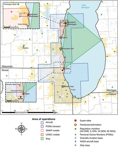
Figure 1 places the two ground-based EM sites in context with the wider LMOS 2017 field campaign. Figure 1 shows nearby EPA AQS monitoring sites; it further shows a campaign-specific network of portable ozone monitors (Model POM, 2B Technologies) installed in Sheboygan. Additional campaign measurements including Pandora solar spectrometers (Herman et al. 2009) and ceilometers (Vaisala CL51) are noted; these were deployed by the EPA National Exposure Research Laboratory (EPA NERL) in collaboration with the Wisconsin Department of Natural Resources (WDNR). Two aircraft flew during the campaign, Scientific Aviation (Conley et al. 2014) and the NASA LarC UC-12, which carried the Geostationary Trace gas and Aerosol Sensor Optimization (GeoTASO) instrument (Judd et al. 2019). The areas of operation for mobile sampling platforms are also shown: the UW-Eau Claire (UWEC) and EPA Region 5 Geospatial Monitoring of Air Pollution (GMAP) vehicle-based samplers operated between Zion and Sheboygan, while an instrumented vessel (NOAA RV 5503) sampled on Lake Michigan. Further description of measurements can be found in the LADCO Synthesis report and recent LMOS 2017 publications.

Figure 1. Overview map showing spatial coverage of LMOS 2017. Green and dark blue polygons indicate ship and aircraft operations areas, respectively. Enhanced monitoring sites at Sheboygan, WI (north) and Zion, IL (south) are mapped in more detail with insets. KUGN station is Waukegan Airport. Source: Wisconsin Department of Natural Resources (WDNR)

Many of the goals listed above concern the spatial representativeness of the LMOS 2017 EM sites. To be most useful in testing models, EM sites should sample air that is representative of larger portions of the airshed (e.g., satellite pixels, PGM grid cells of 16 km² or 144 km²). With the exception of source-oriented sampling (which was limited during LMOS 2017), local impacts should be minimized in site selection, and then characterized to aid in interpretation of model-observation differences. A unique challenge in this context for coastal air pollution is the presence of sharp atmospheric gradients, especially for ozone (Goldberg et al. 2014; Hastie et al. 1999; Stauffer et al. 2015; Sullivan et al. 2018). Ozone concentrations can vary dramatically with distance from the lake shore and due to fine scale features that influence lake breeze meteorology and the development of the thermal internal boundary layer (TIBL) (Lyons and Olsson 1973). These factors include surface roughness, vegetation, topography, angle of shoreline, and shoreline features, such as bays and points.

Source-receptor techniques such as positive matrix factorization (PMF) have become widely accepted tools for characterizing source impacts in routine and campaign field measurements. In this work, we focus on PMF with hourly or sub-hourly input data in order to assess impacts from intermittent and localized sources. This approach has been used with time-resolved aerosol particle size distribution data (Zhou et al. 2004, 2005) as well as with time-resolved volatile organic compound measurements (Abeleira et al. 2017; Zhou et al. 2004, 2005). These studies have been located in metropolitan areas, such as Pittsburgh, St. Louis, or Denver and been successful in identifying emission source groups for traffic, steel processing, sulfate sources, nitrate sources, oil and natural gas, and biogenic sources. Unlike these previous studies, the LMOS EMs are located near a large water body (Lake Michigan) which presents the opportunity to investigate PMF’s ability to identify sources after long-range transport over the lake. We jointly analyze the PMF results with meteorology to calculate conditional probability functions (CPF), which helps localize sources to specific wind sectors (Lee, Hopke, and Turner 2006; Pekney et al. 2006).

Methods

Site selection and description

In order to improve the interpretation of the Zion and Sheboygan ground-based EM sites, site description and selection process are captured in this section. The EM sites are mapped in Figure 2 and more detailed layouts of each site, showing location of key samplers and meteorological instruments relative to buildings can be found in Supplemental Information (SI) Section F.

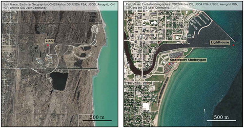
Figure 2. Maps of the EM sites for LMOS 2017 at (a) Zion IL and (b) Sheboygan WI. Also shown is Sheboygan lighthouse, used for supplemental meteorological measurements

Sites at the lakeshore were the highest priority for sampling the polluted air masses coming off the lake before significant growth of the TIBL. In an ideal sampling configuration, these lakeshore sites would be supplemented with additional sites at a range of distances from the lake, including sites on the water using buoys or piers, and sites far enough inland to be out of the lake breeze penetration zone. Due to the resource intensity of this configuration, LMOS 2017 focused on two fixed EM sites and employed alternative approaches to probe meteorological and concentration gradients, including a network of low-cost ozone monitors, aircraft flight paths, and mobile sampling using vehicles with on-board ozone monitors. It is important for EM sites to have relatively minor local source impacts in order to make them as representative as possible for airshed level sampling. Other practical considerations included site security, site access, preexisting measurements, and localized vegetation. Localized vegetation can influence biogenic emissions, obstruct remote sensing equipment, and modify wind fields.

Four additional factors entered into the Zion site selection: (a) coastal site with persistent high ozone design values; (b) VOC sensitivity in transition from the high NO_x urban core to the NO_x limited regional airshed; (c) manageable flight restrictions permitting aircraft-based vertical profiles; and (d) sufficient proximity to Chicago to sample the urban plume at high concentrations, but after mixing in order to avoid plumes from individual sources.

Preliminary data and modeling (Pierce et al. 2016) indicated these conditions would be met at Zion due to its location 67 km north of downtown Chicago. Science flight operations above Zion required permission from Waukegan National Airport; however, Zion was outside the Class B controlled airspace for Chicago O’Hare. The Zion EM site (42.468 N, 87.810 W) was collocated with a routine Illinois monitoring location (AQS 17–097-1007) inside the Illinois State Beach Park 900 m inland from the shoreline. In the AQS database and in previous studies, AQS 17–097-1007 is referred to as the Camp Logan Trailer.

The choice of the Spaceport Sheboygan site was based on several additional factors, including proximity to established monitoring sites, sightlines for remote sensing instruments, and available space and power for two large instrument trailers. Spaceport Sheboygan (43.745 N, 87.709 W) met these requirements, and was located just south of the harbor and centered between two regulatory monitors operated by Wisconsin DNR, Sheboygan Haven (AQS ID 55–117-0009) and Sheboygan Kohler Andrae (AQS ID 55–117-0006). The location was immediately southeast and across the Sheboygan river from the Sheboygan central business district and 240 m from Lake Michigan at its closest point. Also marked in Figure 2b is the location of the Sheboygan lighthouse, which was used as the source of local meteorological measurements. For clarity, all discussion of Sheboygan refers to Spaceport Sheboygan EM site unless noted otherwise.

Both Zion and Sheboygan were measurement sites during LMOS 1991 (Bowne and Shearer 1991). However, the exact measurement locations were different in 1991. Distances between the 1991 and 2017 sites range from 1 to 8 km in Zion and Sheboygan. Furthermore, distances and directions from local sources, and from Lake Michigan, were different during the campaigns.

Data sources

Data used in this paper for EM site characterization are described here. A complete list of instrumentation at the EM sites is available through the campaign repository, and the synthesis report (Abdioskouei et al. 2019).

Zion

In situ gases measured at the Zion site included volatile organic compounds (VOCs) by proton transfer reaction quadrupole interface time-of-flight mass spectrometer (PTR-Qi-TOF, Ionicon Analytik) as described in Millet et al. (2018) and by offline gas chromatography of periodic canister collections (Schauffler et al. 1999), nitrogen oxides (NO and NO₂, Chemiluminescence, Thermo Fisher 42i), ozone (UV Photometric, Teledyne 400E), sulfur dioxide (SO₂, UV Fluorescence, Teledyne 100E), and finally nitric acid (HNO₃) and hydrogen peroxide (H₂O₂) by chemical ionization mass spectrometry (CIMS, Tofwerk AG, Switzerland, and Aerodyne Research Inc., USA) as described in Vermeuel et al. (2019). During LMOS 2017, a semi-continuous gas chromatograph-mass spectrometer (GC-MS) was operated at Zion for hourly analysis of VOCs; however, the data did not pass post-campaign QA-QC intercomparison checks to the PTR-Qi-TOF and to independent VOC canister measurements, and is not used herein.

At Zion, two versions of the NO_x data are available in the repository, which we refer to as NO_x-OVI (outlier values included) and NO_x-OVE (outlier values excluded). The outlier exclusion identified and excluded 1 min datapoints whose absolute deviation from a 5 min moving average exceeded 4.45 times the mean absolute deviation of the 5 min period. The outlier removal removed 11.2% of the 1 minute datapoints in the NO_x-OVI time series. The mean (± one standard deviation) of the NO_x datasets are 2.37 ± 3.59 ppb and 2.17 ± 3.19 ppb for the OVI and OVE datasets, respectively. NO_x-OVE was thought to be more relevant to PGM modelers due to exclusion of local sources capable of short duration excursions; therefore, NO_x-OVE was used in all analyses and statistics except the analysis of NO_x impact from nearby locomotive traffic, which used the NO_x-OVI timeseries.

Fine particulate matter smaller than 2.5 microns (PM_2.5) was collected via integrated aerosol filters (3000B, URG Corporation) and composition analyzed post campaign as described in Hughes et al. (2021). Winds at Zion were measured by the Illinois EPA (IEPA) on a 10 m met tower. Particle size distributions were measured with a Scanning Mobility Particle Sizer (SMPS, TSI 3936) and an Aerosol Particle Sizer (APS, TSI 3321). The size ranges of these instruments, after conversion of aerodynamic to electrical mobility sizes for the APS (Khlystov, Stanier, and Pandis 2004), were 13–562 nm, and 542– 8354 nm, respectively. Instrument-specific time resolutions and representative LMOS 2017 values for select measurements can be found in Table 1. Audio volume measurements were performed during a 10-day subset of the LMOS campaign (192 hours during June 14 – June 23) for detection of trains, which passed Illinois State Beach on a freight and commuter rail line 0.5 km to the west. These were taken at 1 sec time resolution using the microphone of an Android tablet and AirCasting data acquisition software, with the tablet installed in a rainproof box approximately 17 m east of the tracks and 70 m north of 17^th street.

Table 1. Statistics for select measurements from Zion ground site

			Mean		Standard deviation		Median		Interquartile range		n
Variable	Time resolution	Unit	Daytime	Ozone events	Daytime	Ozone events	Daytime	Ozone events	Daytime	Ozone events	Daytime	Ozone events
N0.02–20‡	2 min	cm^-3	5711	9278	4020	4993	4717	8772	4481	7227	6844	1834
Nitric acid	1 min	pptv	839	1226	1100	995	430	876	945	1115	11319	3840
Hydrogen peroxide	1 min	pptv	2062	3432	1939	1925	1365	3400	2651	2621	11319	3840
Ammonium	12 hr	μg m^-3	0.321	0.462	0.178	0.221	0.300	0.388	0.240	0.258	32	8
Nitrate	12 hr	μg m^-3	0.129	0.156	0.152	0.120	0.086	0.120	0.081	0.078	32	8
Sulfate	12 hr	μg m^-3	0.861	1.271	0.470	0.567	0.832	1.113	0.503	0.752	32	8
PM2.5*	12 hr	μg m^-3	5.05	8.24	2.92	2.58	4.08	7.33	3.96	3.92	32	8
Ozone	1 min	ppbv	47	60	14	13	45	62	20	17	14430	3848
Air temp	1 min	C	22.3	26.7	4.3	3.1	21.3	26.5	6.2	4.3	14430	3848
Wind speed	1 min	m/s	5.00	4.42	3.28	1.99	4.60	4.20	3.20	2.70	14430	3848
Relative humidity	1 min	%	56.0	53.8	15.0	14.8	55.0	54.0	24.0	23.3	14430	3848
Nitric oxide^δ	1 min	ppbv	0.43	0.69	0.90	1.27	0.16	0.19	0.32	0.38	15360	3840
Nitrogen dioxide^δ	1 min	ppbv	1.54	3.15	2.91	4.19	0.67	1.44	1.84	2.43	15360	3840
Nitrogen oxides^δ	1 min	ppbv	1.97	3.83	3.73	5.42	0.86	1.60	1.99	2.88	15360	3840
PM2.5†	2 min	μg m^-3	6.38	10.47	4.28	3.90	5.00	9.80	6.20	6.70	7920	1920
PM10†	2 min	μg m^-3	8.27	13.68	5.66	5.33	6.70	12.70	7.80	6.90	7920	1920
Acetone	1 min	ppbv	1.38	2.02	0.54	0.37	1.17	1.96	0.81	0.45	15392	3848
Acetonitrile	1 min	ppbv	0.066	0.089	0.023	0.024	0.061	0.088	0.030	0.029	15392	3848
Benzene	1 min	ppbv	0.050	0.083	0.036	0.036	0.035	0.073	0.042	0.038	15392	3848
C4 carbonyls	1 min	ppbv	0.150	0.249	0.117	0.062	0.105	0.238	0.149	0.088	15392	3848
C5 carbonyls	1 min	ppbv	0.030	0.051	0.019	0.013	0.022	0.052	0.029	0.017	15392	3848
C6 carbonyls	1 min	ppbv	0.012	0.021	0.009	0.007	0.008	0.020	0.012	0.009	15392	3848
Isoprene	1 min	ppbv	0.698	1.56	0.805	0.830	0.351	1.53	0.917	1.06	15392	3848
Methanol	1 min	ppbv	3.99	5.76	1.76	1.58	3.49	5.74	2.04	2.77	15392	3848
Toluene	1 min	ppbv	0.068	0.107	0.087	0.092	0.039	0.071	0.053	0.077	15392	3848
Radiation	1 min	W m^-2	624	670	298	260	688	750	499	343	15500	3840
Sulfur dioxide	10 min	ppbv	0.34	0.40	0.29	0.22	0.32	0.39	0.31	0.27	1282	384

*Measured by integrated filter

†Calculated from particle size distribution

‡Particle number concentration for particles with diameters between 0.02 and 20 microns

^δNO, NO_x, and NO₂ are from the OVE (outlier values excluded) time series (see Methods).

Sheboygan

At the Sheboygan site, nitrogen oxides were measured via chemiluminescence (Teledyne T200U) and ozone via UV absorption (Model POM, 2B Technologies). Surface winds were measured as part of the EPA meteorology suite. Instrument-specific time resolutions and representative LMOS 2017 values for select measurements can be found in Table 2.

Table 2. Statistics for select measurements from Sheboygan ground site

			Mean		Standard deviation		Median		Interquartile range		n
Variable	Time resolution	Unit	Daytime	Ozone events	Daytime	Ozone events	Daytime	Ozone events	Daytime	Ozone events	Daytime	Ozone events
Formaldehyde	1 min	ppbv	1.76	2.55	0.72	0.74	1.57	2.41	0.81	0.68	12755	1920
Formic acid	1 min	ppbv	0.628	1.161	0.505	0.638	0.530	1.040	0.530	0.750	12755	1920
Ozone	1 min	ppbv	45.5	62.8	12.7	12.6	43.6	61.7	17.3	18.6	15360	1920
Nitric oxide	1 min	ppbv	0.703	0.372	0.808	0.678	0.720	0.100	0.600	0.720	15360	1920
Nitrogen dioxide	1 min	ppbv	1.68	2.24	1.18	1.35	1.36	1.74	1.04	1.45	15360	1920
Nitrogen oxides	1 min	ppbv	2.38	2.61	1.77	1.95	2.02	1.84	1.27	2.13	15360	1920
NOy	1 min	ppbv	1.86	3.04	2.18	2.47	1.30	2.10	1.80	2.40	15360	1920
Wind speed	1 min	m/s	17.2	18.9	4.3	3.7	17.1	17.3	4.7	5.0	15360	1920
Air temp	1 min	C	64.7	66.1	15.9	12.2	66.2	68.4	26.9	18.7	15360	1920
Relative humidity	1 min	%	1.76	2.55	0.72	0.74	1.57	2.41	0.81	0.68	12755	1920

In addition to site-specific measurements listed above for the EM sites, a detailed listing of available meteorological measurements within 10 km of each site is found in Table S2 of SI section C.

Ozone episode classification

Site-specific episode days were determined when the maximum hourly ozone concentration was 70 ppb or higher. A set of test criteria were also developed to determine time periods of high ozone concentrations that had a larger spatial coverage, or multi-site ozone episodes. These test criteria are discussed in SI Section A. Daytime hours are defined as 9–5 pm CST and nighttime as 6 pm – 8 am CST coinciding with the analysis in Abdi-Oskouei et al. (2020).

Large point source emissions

Continuous emission monitoring (CEM) system data for Illinois, Wisconsin, and Indiana from the US EPA Air Markets Program Data were used to quantify local industrial and power production emissions from large point sources during LMOS 2017. CEM data included hourly emissions of CO₂, SO₂, and NO_x along with unit-specific information including location and fuel type. Diurnal patterns of NO, NO₂, NO_x, and SO₂ were inspected after segregation of each study hour into one of two categories. In this paper, the term “large point source” refers only to sources whose emissions are tracked by CEM. Category one required the local wind direction to be from (±22.5°) the large point source and the CEM recording greater than 22.7 kg/hr of the pollutant of interest. Category two included all hours not meeting the criteria for category one. Significant differences between diurnal patterns in category one vs. category two were calculated using a pooled two-sample t-test with significance level of 0.05.

Traffic and rail impact assessment tools

The Community LINE source model (C-LINE) and the Community model for near-PORT applications (C-PORT) from the Community Modeling and Analysis System (CMAS) were used for a model-based high spatial resolution estimate of the influence of traffic and rail emissions from nearby roadways and railways on the sampling site (Isakov et al. 2017; Snyder et al. 2013). The model configuration assumed neutral atmospheric stability and summer weekday conditions with westerly wind (major roads are located to the west of the site; Figure 2). Dispersion from these point, line and area sources is then modeled by Gaussian plume formulations (Venkatram and Horst 2006). C-LINE incorporates NEI-2011 v1/MOVES-2014 emissions from arterial roads and highways, but not local roads, in a zone extending 11.5 km to the west of the sites.

Back trajectories

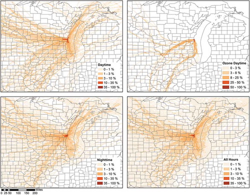
Air mass trajectories were calculated using Hybrid Single-Particle Lagrangian Integrated Trajectory (HYSPLIT) (Rolph, Stein, and Stunder 2017; Stein et al. 2015). Input meteorological fields were from the High-Resolution Rapid Refresh v1 model at 3 × 3 km spatial resolution and 1 hr temporal resolution (Benjamin et al. 2016). Backward trajectories (48 hr in duration) were initialized hourly at 50 m above ground level. Trajectories were converted to spatial density plots, with a 0.05°x0.05° resolution, using m_ij/n_total where m_ij is the number of trajectories passing over grid cell (ij) and n_total is the total number of trajectories.

Factor analysis

Multivariate factor analysis was performed using positive matrix factorization (PMF) using the USEPA PMF version 5.0 tool (Norris et al. 2014). PMF inputs used in this study were gas concentrations and particle size distributions at 10 min time intervals, and uncertainties on those measured values. The PMF technique produces time-invariant factor profiles and a time series of factor contributions. PMF utilizes a stationarity assumption; in other words, emission source profiles are assumed to not change after release. Reactive gases violate the stationarity assumption; gases with a lifetime with respect to oxidation by the hydroxyl radical of less than 8 hr were excluded from the analysis. Consistent with previous studies (Abeleira et al. 2017; Thornhill et al. 2010) NO_x, acetaldehyde, and isoprene were included in the PMF analysis even though they have short lifetimes. An OH concentration of 5 × 10⁶ mol cm^-3 (the 24 hr average simulated OH at Zion from the HRRR-Noah WRF-Chem of Abdi-Oskouei et al. (2020)) was used for the calculation of lifetime. Particle size distributions were pre-processed for suitability with PMF following Zhou et al. (2004) as described below.

Each set of six consecutive size bins were averaged to produce 30 new size intervals from the original 180. Particle growth periods during nucleation events were excluded since such non-stationary violates PMF model assumptions. Growth events were removed using visual inspection assisted by an interactive MATLAB program.

PMF inputs were averaged to a common 10 min interval. Uncertainties provided by instrument PIs in the NASA repository files (MDL and uncertainty) were used as reported (they can be found in Supplemental Information Table S3). Input data were graded according to the signal-to-noise ratio (S/N) calculated for each species. The number of factors and model solutions were evaluated by examining the model goodness of fit parameter Q. Detailed explanation of these methods can be found in the PMF literature (e.g., Norris et al. 2014; Paatero and Hopke 2003; Reff, Eberly, and Bhave 2007).

OH exposure analysis methods

The OH exposure, defined as the time-integrated exposure of air masses to the hydroxyl radical (de Gouw et al. 2017), was calculated using the toluene:benzene chemical clock method (de Gouw et al. 2017; Warneke et al. 2007). The method assumes a consistent ratio of toluene to benzene in emissions, and determines plume age as toluene reacts more quickly than benzene with the OH radical. The equation and rate coefficient used are reported in Supplemental Information Section B (Warneke et al. 2007).

Concentration data analysis during rail locomotive passage

In order to assess the impact of the nearby (540 m to the west) rail line on pollutant concentrations at the Zion EM, each second of the field campaign with audio volume monitoring at the train tracks was classified into a “train passing” or “no train passing” condition. Data processing for this classification was in MATLAB as follows. Files of 1 sec audible volume collected near the rail line were analyzed to identify peaks with volume over 84.5 dB. Visual inspection of the time series was used to eliminate duplicate detections and to identify the first (t₁) and last (t₂) times to exceed 80 dB. After the elimination of overlapping detections, 211 potential train passage detections were identified. Audio data were synchronized with wind, rainfall, NO_x, and particle measurements.

A subset of the 211 train passage detections was identified, based on favorable conditions for transport of pollution plumes from the tracks to the site: wind directions between 188° and 358°, wind speed above 0.75 m/s, no rain, and absence from an exclusion list based on field notes (thunderstorms and inspection periods that might disrupt the audible volume record). The period preceding t₁ by 10 min was used as the “before train” analysis period, although it was shortened if needed based on the previous train’s detection time. We allowed 20 minutes for dispersion of the previous train’s plume. The period from t₂ plus 3 minutes until t₂ plus 20 minutes was used as the 17 min “after train” analysis period. The degree of rail impact on the measurement site was determined by comparison of concentrations before and after the train passage. The 3 min reflects the approximate time required to transit the 540 m distance from tracks to the site. Train type was determined by duration of high audio volume, with commuter trains less than 20 sec, and freight trains as greater than 20 sec. Timing guidelines and thresholds were developed based on visual inspection of the time series in conjunction with field notes. Statistical significance of changes in NO_x and particle counts were determined by creating a distribution of paired differences (before train, after train), and then using a paired t-test to test for difference at the 0.05 significance level.

Results and discussion

The Results and Discussion begins with overview and summary of measurements from the EM sites during LMOS 2017, in the context of ozone episodes and their associated meteorology. Analysis of local winds and back trajectories follow. Potential sources are then quantified for source categories that could be assessed at both EM sites (C-PORT, C-LINE model results, and large point source emissions). Subsequent sections focus on source characterization analyses (factor analysis, rail impact, and OH exposure analysis) that were performed only at the Zion EM site, due to its greater availability of high time resolution measurements.

Site overview of ozone air pollution and air pollution meteorology

Three multi-site ozone episode periods occurred during LMOS 2017, denoted periods A, B, and C by the LMOS 2017 team (Hughes et al. 2021). Period A occurred during June 2–4 with the highest, most spatially extended ozone concentrations on June 2. Periods B and C occurred during June 9–12 and June 14–16, respectively. Site-specific high ozone days were June 2, June 4, June 10–12, and June 14–16 (Zion) and June 2, June 11–12, and June 16 (Sheboygan). All further discussion of ozone event days will be of the respective site-specific ozone days. As Tables 1 and 2 show, daytime ozone during all LMOS 2017 campaign daytime hours averaged 47 ppb and 45.5 ppb at the Zion and Sheboygan EM sites, respectively. During the ozone episode daytime hours, the ozone concentrations were 60 ppb and 63 ppb at Zion and Sheboygan, respectively. During daytime hours of ozone episodes, NO_x concentrations at the sites were 3.83 and 2.61 ppb at Zion and Sheboygan, respectively. Typical daytime concentrations of other species used in analysis in this paper can be found in Tables 1 and 2.

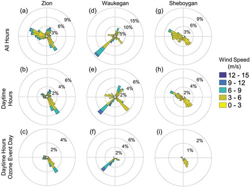
LMOS 2017 period wind roses for Zion, Waukegan Airport (KUGN), and Sheboygan (Figure 3) show frequent winds from the southwest at Waukegan (5.1 km from Lake Michigan). This behavior reflects the most common regional wind condition during summer. This is in contrast to the south and southeast (onshore) winds and westerly (offshore) winds at the coastal Zion (0.9 km from lake) and Sheboygan (0.2 km from lake) sites. Roses are separated by period: all hours, daytime, and daytime on ozone episode days. The wind roses show that coincident occurrence of onshore daytime lake breeze and high ozone episodes occurred frequently during LMOS 2017. The ozone episode daytime roses indicate onshore lake breeze flows during almost all episode hours at the lakeshore sites (c and i) but not at the more inland site (f). Although Zion (0.9 km from lake) and Waukegan (5.1 km from lake) are only 7.0 km apart, the difference in winds is attributable to the greater number of hours with lake breeze penetration to Zion (0.9 km) vs. Waukegan (5.1 km). Sheboygan, like Zion, experienced frequent onshore (SE) and offshore (W) winds during LMOS 2017. Lake breezes are not usually perpendicular to the shoreline due to the Coriolis effect and the position of the daytime mesohigh that drives lake breeze circulation (Lyons and Olsson 1973).

Figure 3. Wind roses of Zion (left), Waukegan (center), and Sheboygan (right) for the three cases: all hours (a, d, g), daytime hours (b, e, h) and daytime hours during ozone episodes (c, f, i). Wind speed in m/s. Zion: 1-min resolution data from May 31 to June 21. Waukegan: 1 hr resolution data from May 31 to June 21. Sheboygan: 1 min resolution data from May 21 to June 21

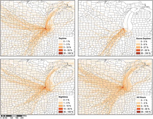
To add longer range transport perspective to the locally focused wind roses, backward air mass trajectories are used. Figure 4 shows the spatial density plot of 48 hr back trajectories ending at Zion for the LMOS 2017 period. These are consistent with the wind roses from Figure 3. Nighttime trajectories (Figure 4c) have a higher frequency of southwesterly winds compared to the daytime trajectories (Figure 4a), which have higher northerly and south-easterly frequency. Lake breeze influence is seen in daytime Zion site-specific ozone episodes (7 days, Figure 4b). Trajectories for lake breeze periods are often curved, as synoptic flow from the SW and nighttime offshore lake breezes are gradually turned during the lake breeze setup, and finally brought onshore in SE flow. Our segregation of data into daytime hours (Methods) captures some hours before lake breeze setup in the daytime figures; these hours still have offshore or synoptic southwesterly flow on most of the ozone days. This is known from more detailed analysis of the timing of lake breeze onset on specific ozone event days (Abdi-Oskouei et al. 2020), where the average lake breeze arrival time at Zion and Sheboygan were 10:38 am and 9:32 am CST, respectively, as described in Wagner et al. (2021).

Figure 4. Spatial density plot of 48 hr back trajectory frequency for trajectories terminating at Zion, grouped by (a) daytime, (b) ozone episode daytime, (c) nighttime, and (d) all hours

Similarly, Figure 5 depicts the trajectories terminating at Sheboygan. Figure 1 illustrates that southerly flows at Sheboygan will arrive after passing over the lake. Daytime hours (Figure 5a) have high prevalence of distinct lake (southerly) and westerly winds; however, nighttime hours (Figure 5c) do not have a prominent direction. Yet, during daytime hours of site-specific ozone event days (4 days) the lake influence is more frequent (25–50% of trajectories) than when considering all daytime hours (13% of trajectories).

Figure 5. Spatial density plot of 48 hr back trajectories for trajectories terminating at Spaceport Sheboygan for (a) daytime, (b) ozone daytime, (c) nighttime, and (d) all hours

Dependence of O₃ and NO_x on wind direction during LMOS 2017 at the EM sites is shown in pollution roses (Figures 6 and 7). Pollution roses are similar to wind roses, except pollution concentration is plotted in place of wind speed. Figure 6 employs the NO_x-OVE data to deemphasize local sources, although matching figures from NO_x-OVI dataset (Supplementary Information S14) have only minor changes in the relative frequency of high NO_x, with a shift of highest NO_x periods from SE (down from 7% to 6%) to W (up from 6.5% to 7.5%). The all-hours plots (a,d) show that O₃ and NO_x enhancements both originated primarily from the southeast and west during LMOS 2017, with the highest concentrations occurring during SE winds. The daytime plots (b,e) reveal minimal westerly influence and show the influence of lake breezes with higher NO_x and O₃ concentrations during the day; elevated NO_x and O₃ in westerly winds are therefore associated with nighttime winds at these sites. CPF plots for each case using threshold values of 70 ppb for O₃ and 15 ppb for NO_x, confirm enhancements originate from the southeast. CPF plots are located in Supplemental Information Section G.

Figure 6. Pollution roses for O₃ (left) and NO_x (right) at Zion site grouped by (a, d) all hours, (b, e) daytime hours and (c, f) ozone episode daytime. Concentrations in ppb. Created using 1 min resolution data from May 31 to June 21

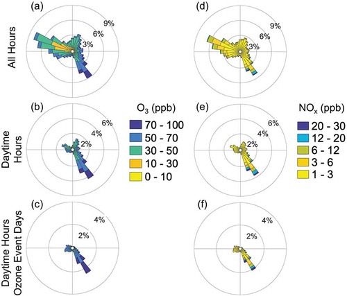
Figure 7. Pollution roses for O₃ (left) and NO_x (right) at Sheboygan site grouped by (a, d) all hours, (b, e) daytime hours and (c, f) ozone episode daytime. Concentrations in ppb. Created using 1 min resolution data from May 21 to June 21

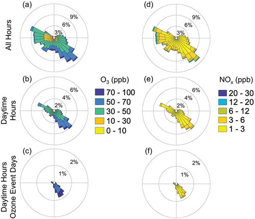
Sheboygan pollution roses were created for the same three cases: all hours (a, d), only daytime hours (b,e) and daytime hours on ozone episode days (c, f). Figure 7 shows that plumes arriving at Sheboygan with high levels of O₃ during LMOS 2017 originated primarily to the south and southeast of the site (as also seen at Zion). During daytime, Sheboygan experienced both southeasterly and westerly winds, but during daytime on ozone event days winds were almost exclusively southeasterly. The NO_x roses at Sheboygan are similar to those for Zion except that concentrations of greater than 20 ppb were not observed.

A majority of the high ozone days sampled during LMOS 2017 corresponded to local lake breeze conditions, consistent with findings from past studies around Lake Michigan (Lennartson and Schwartz 2002). Additional information on meteorological remote sounding results from Zion and Sheboygan during LMOS 2017 can be found in Wagner et al. (2021). Additional discussion of the sensitivity of air quality predictions to lake breeze skill during LMOS 2017 can be found in Abdi-Oskouei et al. (2020).

Source impacts

Local (<15 km) sources can be challenging for model-observation interpretation, as they may be sampled before appreciable dilution, but modeled using instantaneous dilution across the full model grid volume in PGMs. Furthermore, intermittent sources such as festivals, fireworks usage, and other public gatherings may influence a measurement location but be absent from emission inventories. Finally, temporal profiles of emission inventories are based on average activity patterns, and substantial variation can occur due to holidays, business and school closures, unusual traffic patterns, and weather influences on combustion, recreation, and travel patterns. In this section, we discuss traffic, rail, and large point sources that may be relevant to data interpretation at the LMOS 2017 EM sites.

Potential local source impacts

At the Zion site, this included vehicles, a recreational marina, nearby homes and businesses, within-park camping, and the local rail line. The Zion site was located roughly 1.3 km from a busy arterial road (IL 137, Sheridan Rd., 4–5 lanes, undivided), 0.5 km from a local rail line, and 1.6 km from a nearby marina. Within the park, visitor’s vehicles, campfires, and grills were identified as potential sources. Residential emissions of VOCs, nitrogen oxides (NO_x), and PM_2.5 were expected from consumer product use, fuels, and biomass burning. Additionally, three power plants equipped with CEM monitoring were located within 15 km of the Zion site.

Sheboygan included active construction, a recreational marina and harbor, and traffic from a local resort. Spaceport Sheboygan was located on a small peninsula created by the Sheboygan River (190 m south and 180 m west) and Lake Michigan (240 m east), across the street from the Portscape Apartments and Blue Harbor Resort, 590 m southwest of the Sheboygan Harbor, and 260 m southeast of a boat charter on the Sheboygan river. Local emissions of VOCs, NO_x, and PM_2.5 were expected from businesses, apartment complex, and resort located on the peninsula. Additionally, one power plant was located 3.5 km south of the site.

Traffic impacts

Traffic impacts from arterial and larger roads within 11.5 km were assessed using the C-LINE model as described in Methods. C-LINE results for Zion averaged 0.019 μg m^-3, 0.92 ppb, and 0.23 ppb for PM_2.5, CO, and NO_x, respectively. The closest modeled road was Sheridan Rd. (IL 137) 1.3 km from the site. Local roads and the park access road were not included in the C-LINE estimate. For Sheboygan, arterial roads contributed 0.020 μg m^-3, 1.34 ppb, and 0.23 ppb to PM_2.5, CO, and NO_x, respectively. The mean measured NO_x concentrations at Zion and Sheboygan over the campaign were 2.17 ppb and 3.35 ppb, respectively. Expressed as a percentage, under westerly winds and neutral stability, arterial roads and highways would contribute less than 11% of average NO_x at both locations.

Large point source impacts

Cartograms of CO₂ emissions from large point sources during the field campaign are shown in Figure 8. The cartogram is constructed to show the logarithm of distance from the EM site to CO₂ sources. Circular marker area is proportional to the cumulative emission during the campaign. State borders for Wisconsin, Illinois, Indiana, and Michigan are shown in solid lines and their distortion is due to the logarithmic scale used. An asterisk at the center marks EM site locations.

Figure 8. Cartograms centered on (a) Zion and (b) Sheboygan showing location and cumulative emissions (CO₂) of major stationary sources relative to the EM sites. Cartograms are scaled according to logarithm of distance away from the EM site

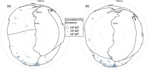
Figure 8 shows that the two EM sites are not close to the highest emitting stationary sources, which are mainly in the Ohio river valley. The location of power plants within 15 km of the EM sites is shown in Figure 9, with CO₂ emissions during LMOS 2017 proportional to the circles marking the sites, and NO_x and SO₂ emissions during LMOS 2017 shown as bar graphs near each source.

Figure 9. (a) Pleasant Prairie, (b) Zion Energy Center, (c) Waukegan Generating Station and (d) Edgewater Generating Station. Areas of circles are proportional to facility CEM cumulative CO₂ emissions and bar charts of cumulative NO_x and SO₂ emissions (MT) during LMOS 2017 from May 21 to June 21

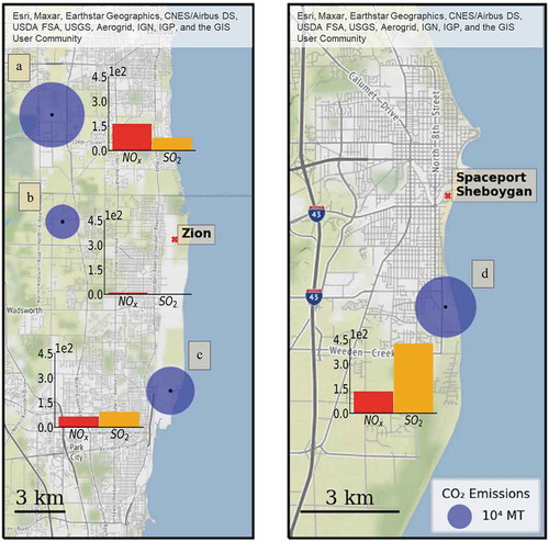
For Zion, two large point sources within 10 km operated during LMOS 2017. To the northwest, at a distance of 6.12 km, is the Zion Energy Center. Zion Energy Center had three natural gas boilers, each reporting CEM emissions. The boilers had similar emissions when operating (approximately 90 metric tonnes (MT) of CO₂ per hour), but had different operational schedules during LMOS 2017 (daytime only, intermittent use, etc.).

To the south of the site, and within 10 km, is the Waukegan Generating Station (WGS). WGS is located directly on the Lake Michigan shoreline 7.17 km from the Zion sampling site. Waukegan has 6 CEM units (four diesel and two coal). The four diesel units operated for only a few hours during LMOS 2017 and are not considered further herein. One coal-fired unit was shut down until June 12, and then operated on a diurnal cycle with peaks during the daytime of approximately 270 MT/hr CO₂. NO_x and SO₂ emissions were significant, typically peaking at 135 and 450 kg/hr, respectively. The second coal-fired unit at WGS had a similar diurnal cycle and emission amount, but operated at its usual rate during only 50% of the study days. While the most common wind frequency during daytime ozone episodes at Zion was from the southeast (and not the south), winds sometimes rotated from SW to SE as the lake breeze set in during LMOS as shown in Abdi-Oskouei et al. (2019). Thus, some influence from WGS could be expected during portions of ozone episodes at Zion during LMOS 2017. This is further supported by the non-zero frequency to the due south of Zion in the spatial density plot of back trajectory frequencies (Figure 4b).

A larger emission source was located at 11.7 km to the northwest of the site: the Pleasant Prairie coal-fired power plant. Pleasant Prairie had two CEM-tracked units operating during LMOS 2017 and was not located upwind of Zion during ozone episodes. The first of these was down until June 1. It subsequently operated with a diurnal cycle that peaked in daytime at about 635 metric tonnes CO₂ per hour and had a minimum in the early morning of about 450 metric tonnes per hour. SO₂ and NO_x emissions were appreciable, peaking at approximately 90–160 kg/hr and 180–230 kg/hr , respectively. Pleasant Prairie #2 is similar to the first unit, but switched from idle to operational on June 8. Both units had elevated SO₂ emissions (about twice the normal daily peak) occurred for approximately 36 hours centered on June 12. Pleasant Prairie and Zion Energy Center also had occasional hourly enhancements in NO_x emissions above typical peak values, often at startup.

For Sheboygan, one large point source nearby to the EM site operated during the campaign (Figure 9). Edgewater Generating Station was located 3.5 km south of the Sheboygan site and had two coal fired units in operation during LMOS 2017 which were upwind of the site during ozone episodes. These operated on a diurnal cycle with a peak of 720 metric tonnes CO₂ per hour and a minimum of about half the peak level. Peak SO₂ and NO_x emissions were about 790 and 270 kg/hr, respectively, with disproportionate emissions of these from unit one. Operation was consistent throughout the campaign except for a few days of half-capacity operation.

As a quantitative test of significant impact from the power plants discussed above, measured diurnal profiles of pollutants were analyzed jointly with local wind directions as described in Methods. We note that the absence of a statistically significant impact using this method is not the same as verification of zero impact or quantification of impact. However, the simple comparison of concentrations segregated by wind direction and CEM emission rate should detect large direct impacts from the nearby large point sources. At Zion, SO₂, NO, NO₂, and NO_x measurements were analyzed. Comparison of diurnal patterns for SO₂, NO, NO₂, and NO_x did not show statistically significant differences, suggesting that SO₂ and NO_x variability at Zion was mainly driven by sources other than local power plants. Diurnal patterns for Zion (Figure S1) are located in supplemental information section D.

At Sheboygan, NO, NO_x, and NO₂ measurements were analyzed. For Sheboygan, Edgewater routinely emitted over the 22.7 kg/hr NO_x threshold. However, NO was significantly lower with winds from Edgewater (p = .0024), while the other compounds had insignificant differences. We interpret this as a symptom of the coincidence of lake breeze winds with the Edgewater power plant. As Figures 1 and 4 show, winds from the due south at Sheboygan EM site can be coincident with the Edgewater station. During these periods, a number of long-range and localized source influences are possible, including the Edgewater station. Our interpretation and lessons learned from this are threefold. First, site placement in future campaigns should avoid this type of directional coincidence. Second, as Edgewater during LMOS 2017 emitted SO₂ at a rate of 13.24 MT/day (Figure 9), the lack of in situ SO₂ monitoring at the Sheboygan EM site was a missed opportunity to characterize plume influence. Third, additional analysis using LMOS aircraft spirals, wind and temperature profiles taken at Sheboygan, comparison of Kohler Andre and Sheboygan pollutant concentrations, and/or plume resolving dispersion models such as SCICHEM (Chowdhury et al. 2015) may be appropriate for further interpretation of the LMOS 2017 measurement record. Diurnal patterns for Sheboygan (Figure S2) are located in supplemental information section D.

Particle measurements (Zion)

At Zion, the full aerosol size distribution from 1 nm to 8.35 µm (aerodynamic diameter) was measured with two SMPSs and an APS; here we use the size distribution from 13 nm to 8.35 µm. Descriptive statistics of the particle size distribution measurement were number concentrations of 5268 cm⁻³ (15–100 nm size range), and 6335 cm⁻³ (15–2500 nm size range). The inferred PM_2.5 from the size distribution measurement was 6.36 µg m⁻³, which compares favorably to the gravimetric co-located filters which measured 5.2 µg m⁻³. The mode of the mean number-size distribution was 40 nm and bimodal mean volume size distributions peaked at 223 nm and 2.661 µm. Ultrafine particle burst events were identified qualitatively and occurred on 14 days of the campaign, with nearly all events beginning in the morning between 10:00 am – 1:00 pm CST.

Rail impact (Zion)

In order to better quantify the impact of rail on the site, audio volumes were recorded for 192 hours during the period June 14 – June 23, as described in methods. The rail line 540 m to the west was used for Metra commuter trains, and for Union Pacific freight. After filtering for appropriate wind speed and wind direction (see methods), pollutant measurements at Zion (NO, NO₂, NO_x, and particle size distribution) were then compared for the periods prior and after the train. Ninety-four train detections met analysis requirements (sufficient pollutant measurements, suitable meteorology). Inspection of aerosol size distributions showed the strongest signal in the 15 to 30 nm range (N_15-30). As shown in Figure 10, N_15-30 increased after trains passed, rising from an average pre-train value of 2024 cm⁻³ to an average post-train value of 2510 cm⁻³. Individual cases were often more sharply featured, with a distinct plume of 3–10 min duration at the Zion site. The broadening of the peak in Figure 10a arises from the variability in timing and shape of these plumes over the 94 cases. Figure 10b shows the distribution of concentrations before (blue) and after (orange) the train, with the post-train appearance of a tail at concentrations in excess of 7000 cm⁻³. Figure 10c shows that the pre-train (blue) and post-train (orange) audible volumes follow the same distribution with a mean of 58–59 dB. The increase in particles at the 15–30 nm size range was significant (p = .0029).

Figure 10. Results from 94 train detections over a 10 day period meeting all required criteria (meteorology and available particle size distribution measurements). The average time series is shown in panel (a) with a short pulse of audio volume indicating passage of train; particle number increases, rising from a minimum of 1930 cm^-3 to a peak of 2749 cm^-3 5.5 minutes after the train detection. Histograms of (b) particle number and (c) audio volume before and after show modest increase, and no change, respectively

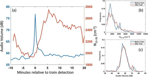
Similar analyses were done for particle mass below 0.5 µm, NO, NO₂, and NO_x, with analyses also performed separately for commuter (91 detections with suitable meteorology) and freight (20 detections with suitable meteorology). Statistically significant (one-sided p-value < 0.05) increases were observed for particle number for all trains, particle number for commuter trains, NO for all trains, and NO for commuter trains. NO increased from 0.33 ppb (pre-train) to 0.42 ppb (post-train) on average. Unlike the N_15-30 increase, which was detected with many (but not all) trains, the NO increase distribution was more skewed due to a small number of high concentration plumes, possibly indicating high emitting trains or intermittent high emitting conditions for NO. Increases in NO_x, NO₂, and particle mass <0.5 µm were observed on average but were not statistically significant at the 0.05 level. The Metra trains were reported to be over 88% tier 0 and tier 0+ in 2018 (Victory 2018). Tier 0 is higher emitting compared to new (tier 4) heavy duty diesel engines.

Some false-positive train detections are likely, due to extraneous sources of high volumes, such as thunder, rain, and wind. The frequency of train detections, after removing rain periods (7 train detections) and other known events was 26.3 per day, which exceeded the number expected based on the Metra schedule and reports of freight activity. Freight activity was estimated (M. Harrell, email to C. Stanier, June 8, 2017). In total, we expected an average of 21 train detections per day. The additional 5.3 may be false positives (and therefore the emission per train would be biased low) or they may reflect a low a priori estimate.

Each train passage happens quickly; therefore, the perceived impact on air quality may be limited. However, our 17 min post-train averaging period multiplied by 26.3 trains per day corresponds to 31% of an average day impacted at the levels reported above. Thus, at 540 m distance from the rail, approximately 7% of the 24 hr average N_15-30, and 1% of the 24-h average NO_x, may be from rail traffic even though the source is present for only minutes at a time.

Although we are not able to recover emission factors, and thus cannot compare directly to EPA heavy-duty diesel standards, we can compare to modeled local impacts (C-PORT) and to published ratios of emission factors, such as PM_2.5, number, and NO_x emission factors (Johnson et al. 2013). The NO_x impact under neutral westerly winds (0.051 ppb) from the C-PORT model is similar to our measurement (0.028 ppb) considering the limitations and assumptions of the techniques. The corresponding C-PORT PM_2.5 value was less than 0.01 μg m^-3. Although the analysis detected no statistically significant increase in PM_2.5, given the size of the dataset and variability observed, an impact of approximately 0.12 μg m^-3 or larger would have been detectable.

Comparing to measured emission ratios, the NO_x:particle ratio was 1.35 ppb per 1000 cm⁻³ (Johnson, 15–500 nm) compared to 0.19 ppb per 1000 cm⁻³ (this work, 15–30 nm). The PM_2.5:number ratio was 0.065 μg m^-3 per 1000 cm⁻³ (Johnson, 15–500 nm). In our work (on average) a statistically significant PM_2.5 increment from trains was not detectable, and we estimate the detection limit was 0.39 μg m^-3 per 1000 cm⁻³ given the number of samples and observed variability in ultrafine and accumulation mode particles. It should be noted that this is based on a small sample, and may not be representative of average emissions across all long-haul commuter and freight trains in the region; however, these analyses of rail passing do serve as a component of site characterization, inform the interpretation of LMOS data, and provide a rare assessment of in-use rail impact.

Positive matrix factorization results

PMF analyses were conducted for Zion in order to consolidate information from many time-resolved measurements into a smaller number of factors associated with source categories. A parallel analysis for Sheboygan could not be conducted due to the lower number of species measured there. At Zion, two analyses were conducted: one was based on time-resolved gas measurements only; the second included all gases from the first analysis as well as hourly averaged particle size distributions spanning 12.6– 610 nm particle diameter. Our conclusions about source factor contributions presented here are mainly drawn from the gas-only analysis, with some discussion of additional information content with the addition of particle size distribution data.

One goal of our PMF analysis was to resolve local sources that might vary at hourly or sub-hourly time scales. To do this requires using high time resolution data (10 min time resolution data are used herein). This excluded using PM_2.5 metals and organic molecular markers in aerosols that have high resolving power, but that were only available at ~12 hr time resolution as they were collected using filters and analyzed offline.

The PMF analysis identified primary and secondary influences on the site with distinctive diurnal patterns. Factors are named according to the species which loaded most heavily onto each factor. These are (1) SO₂, (2) BTEX (benzene, toluene, ethylbenzene, xylenes), (3) oxygenated VOCs (OVOCs) without acetonitrile, (4) NO_x, (5) isoprene, and (6) OVOCs with acetonitrile. Six factors were used in the analysis because this resulted in a Q/Q_exp ratio closest to one while showing agreement between observed measurements and predicted concentrations when evaluating timeseries and scatter plots for each modeled species. PMF analyses using five, six, and seven factors resulted in Q/Q_exp values of 1.40, 1.07, and 0.93, respectively. Key results from the interpretation of PMF factors include division of factors into mostly primary factors (SO₂, BTEX, isoprene) and those with mixed primary and secondary characteristics (OVOCs, OVOCs with acetonitrile, and NO_x). Features leading to classification as primary emissions were: (i) the dominant species was a primary emission (SO₂, BTEX, isoprene), (ii) the factor was highly correlated with factors thought to be primary; (iii) the diurnal pattern had a peak during nighttime or early morning. An exception to the diurnal pattern test is for isoprene, which is known to peak at around solar noon due to light and temperature-dependent biogenic production. Features leading to classification as secondary included (i) correlation with high ozone periods; (ii) inclusion of compounds known to be formed in atmospheric chemical reactions; (iii) diurnal patterns peaking in afternoon and early evening; (iv) correlation with periods of high photochemical age. Factors can also be divided into those occurring in lake breezes (NO_x and isoprene factors) versus the other factors with primarily west and northwest non-lake breeze impact. Diurnal patterns, directional dependence, relation to ozone episodes, and possible sources of factors are discussed below. Diurnal patterns are located in Supplemental Information Section E.

Time series and CPFs for each factor are shown in Figure 11. The SO₂ factor follows a diurnal pattern with peak levels at 6:00 am CST. The CPF of the SO₂ factor shows a mix of directions with high SO₂, but the southeast is absent; we conclude that the lake breeze ozone episodes at the Zion EM during LMOS 2017 were not enhanced in SO₂ or in fresh emissions from coal-fired combustion. This can be contrasted with the NO_x factor, which often was enhanced in lake breezes, in addition to influences from other directions discussed below.

Figure 11. PMF factor time series and conditional probability functions. Abscissa units are in CST and tick marks are at midnight CST. The shading represents ozone event days

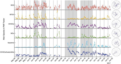
The BTEX factor had high nighttime concentrations during the first portion of the campaign (through June 6). Enhancement of anthropogenic compounds at Zion, particularly in the earlier portion of the campaign, has been noted in Vermeuel et al. (2019) and Hughes et al. (2021). In this pre-June 6 period the BTEX factor was highly correlated with the OVOCs without acetonitrile factor and the CPFs for both show a western sector suggesting coincident origin. The highest concentration OVOC in that factor included acetaldehyde and 4–6 carbon carbonyls. BTEX and OVOC factors in the first period both follow a diurnal pattern with peak levels at midnight and early morning. The PMF technique cannot easily separate small local (i.e., <10 km) from larger more distant sources. The diurnal pattern probably rules out activities within the state park. However, there is likely some contribution from nearby residential and vehicle sources, as well as from numerous more distant sources. The counties to the west and northwest in Illinois (Lake and McHenry) and Wisconsin (Kenosha, Racine, Walworth, Waukesha, Jefferson, and Rock) have high to moderate populations (and therefore on-road and off-road vehicle use). They also include numerous stationary sources. These include many airports, landfills, and VOC emitters of greater than 10 tons per year. Industrial and manufacturing emitters of VOCs in these counties include paint, adhesives, chemical manufacturing, printing, and manufacturing of machinery, glass, plastic, and metal components. Therefore, a mix of combustion and primary factors in offshore nighttime breezes from the west is consistent with the known land uses and known sources in that direction.

During the second period of the campaign (post-June 6), peak contributions of the NO_x factor decreased substantially. A transition to greater secondary and biogenic influence is supported by the isoprene factor. In the first period, the isoprene factor was minimal with the exception of a peak in the early afternoon of June 4. The isoprene factor had influence from both the west and from the southeast (lake breeze). However, on June 4, only westerly winds were observed at Zion, meaning that the afternoon isoprene peak originated from the land west of Zion rather than from the lake breeze.

PMF identified a second OVOC factor that included acetonitrile. The other leading compounds loading onto this factor were acetone and methanol. This OVOC factor had low correlation with BTEX, NO_x, and the other OVOC-dominant factor in either period of the campaign. This factor peaked during ozone episode B on June 10–11 and the CPF indicates a southwesterly influence. In Hughes et al. (2021) this period is shown through back trajectory analysis and organic aerosol molecular markers to have influence from forested areas in Missouri and Arkansas, and to have high secondary organic aerosol (SOA) fraction. Furthermore, it had uniquely high loadings of isoprene organosulfates such as methyltetrol sulfate and glycoloic acid sulfate. Acetonitrile is a marker of biomass burning (de Gouw et al. 2003; Yuan et al. 2010) and NOAA NESDIS HMS analysis of visible smoke and fire detections reveal agricultural burning during June 7–10 along the Mississippi river valley in Arkansas, Tennessee, and Missouri. However, the PM_2.5 levoglucosan timeseries in Hughes et al. (2021) and the OVOC/Acetonitrile factor from this work do not peak on the same days; therefore, attribution of this factor to either fresh or aged biomass burning is uncertain.

PMF analysis for the gases above supplemented by particle size distributions spanning 12.6– 610 nm yielded qualitatively similar results (see Figure S4). In other words, the inclusion of the size distributions did not lead to additional interpretable factors. The best solution included seven factors. These included OVOCs with acetonitrile, NO_x and toluene, isoprene, and SO₂ dominant factors. A particle mode of 160 nm diameter loaded onto the SO₂ dominant factor, and a particle mode of 300 nm diameter loaded onto the isoprene-dominant factor. Three particle modes were identified by PMF without appreciable loading of gases – these were a nuclei mode of 15 nm, and two ultrafine modes at 30 and 80 nm. Since in section 3.4, we showed that 15–30 nm were a marker of locomotive exhaust at Zion, the lack of gases loading onto the 15 and 30 nm dominated factors is further support that the NO_x impact from locomotives is small. And it is further evidence that VOC and OVOC gases are not in the locomotive exhaust. This is helpful from a model-observation comparison standpoint, as intermittency and proximity of the locomotive emissions would be difficult to represent for the Zion site.

Nostalgia Days, a local festival and car show held annually, occurred in Zion on June 16 and 17. It included events such as outdoor music, food vendors, a car show focusing on vintage cars, and parade of cars. The center of activities for Nostalgia Days was in downtown Zion along Sheridan Rd. (IL 137). This is located about 2.35 km from the site to the southwest.

The impact of Nostalgia Days on the Zion measurement record was detectable, but much lower than its maximum potential impact, due to variable winds during Nostalgia Days. On June 16 and 17, daytime winds were from the southeast, and nighttime winds were from the west. During the Nostalgia Days period, increased correlation was observed between three factors consistent with internal combustion and biomass burning. These were the factor with high loading of the 80 nm particle mode, the SO₂/160 nm particle factor, and the factor with OVOCs and acetonitrile. Hughes et al. (2021), with 12 hr PM_2.5 filters analyzed for molecular marker tracers, identified high concentrations of combustion markers on the night of June 16 and the afternoon on June 17, further supporting the influence of Nostalgia days on the Zion measurement site. However, many of the emissions from Nostalgia days likely did not impact the Zion measurement record due to wind direction.

The PMF analysis confirms other assessments about the Zion site during LMOS 2017 from the complementary methods; however, the PMF analysis is the only one to simultaneously consider the VOC and OVOC gases together with SO₂, NO_x, and particles. The main conclusions derived from PMF, or supported by PMF, are that the Zion site is strongly impacted, particularly in daytime, by relatively aged and well mixed plumes of NO_x, OVOC, and secondary particulate matter. These originate at times in a SE lake breeze, and at other times in synoptic SW flow. Peak contributions in secondary factors occurred during episode B (June 10 and 11). Factors that are primary, with the exception of isoprene, are detected mainly at night and in offshore flows with W and NW origins. A split in the campaign into a more primary pollutant phase (before June 6) versus a more biogenic and secondary pollutant phase (after June 6) is supported by PMF, where primary factors (BTEX, NO_x) decrease, the isoprene factor increases, and correlation between OVOCs and BTEX decreases. Nearby primary sources that potentially could have influenced the Zion site, causing problems for model-observation comparison due to model representation issues, are not identified by PMF. This is supportive of their small influence as identified by other means, such as the local traffic impact being less than 11% of average NO_x, and the absence of a detectable influence on diurnal patterns of SO₂ and NO_x depending on large point source emission rate and local winds.

OH exposure

The OH exposure of air sampled at Zion was calculated according to the measured ratio of toluene and benzene as described in Methods and in Supplemental Information. Photochemical age analysis was only performed for Zion as toluene and benzene were not measured at the Sheboygan site. The emission ratio of toluene to benzene was set equal to 2.81 and was determined by taking the 95^th percentile of the measured toluene to benzene ratio from 5 to 9 am for all days of the campaign.

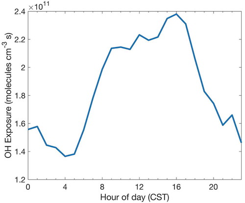
The median OH exposure at Zion, as shown in Figure 12, was 1.9 × 10¹¹ molecules cm⁻³ sec; the maximum exposure observed was 4.8 × 10¹¹ molecules cm⁻³ sec. The diurnal pattern of OH exposure, as shown in Figure 13, peaks at 4 pm CST and has a nighttime minimum. The box plots of Figure 12 show OH exposure distributions for all hours, all daytime hours, all nighttime hours, as well as for daytime and nighttime hours on each ozone episode day. Daytime hours have higher OH exposure than nights, as expected. On average, episode periods have OH exposure distributions similar to the campaign average. Ozone episode days that stood out in terms of OH exposure were June 10, 11, and 16. June 10 and 11 were discussed above due to possible smoke influence, high SOA, and isoprene organosulfate loadings, and long-distance transport from the south and southwest. June 14 stands out as an episode day with a low benzene-toluene OH exposure.

Figure 12. OH exposure (Zion, IL) boxplot for various periods of LMOS 2017. Red line is median; box encompasses 25th to 75th percentiles; whiskers terminate at median ± 1.5 IQR (interquartile range). Red crosses are outliers

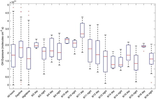
Figure 13. Diurnal pattern of OH exposure

Conclusions

We have provided a comprehensive characterization and documentation of the two main ground-based enhanced monitoring sites (Zion and Sheboygan) from LMOS 2017 which will aid in future interpretation of measurements in the campaign repository, and in planning and execution of future field campaigns.

Both sites allowed investigators to sample, during daytime, polluted lake breezes along the Lake Michigan shore with high concentrations of ozone and NO_x. During daytime hours (9–5 CST) of ozone episodes, Zion had NO_x concentrations (mean ± standard deviation) of 3.83 ± 5.42 ppb, and mean nitric acid concentration of 1.2 ± 1.0 ppb. The corresponding NO_x concentrations at Sheboygan were 2.61 ± 1.95 ppb (nitric acid concentrations were not measured but NO_y averaged 3.04 ppb, implying 0.43 ppb of NO_x oxidation products). Thus, Zion did encounter higher average and peak NO_x and NO_y concentrations, consistent with a stronger impact of the combustion sources and periodic impact of relatively high NO_x plumes. Ozone episodes were divided into periods A, B, and C to aid in future analysis. The LMOS 2017 data are publicly available in a campaign repository, and this paper will facilitate informed use of the data from the Zion and Sheboygan EM sites.

While large point sources emitting NO_x and SO₂ were present close to the monitoring sites (at a distance of 3–12 km), analysis of diurnal NO, NO₂, and SO₂ (at Zion) and NO and NO₂ (at Sheboygan) patterns stratified by CEM emission rate and local winds did not detect a significant impact. This presumably reflects the combined effects of dilution, wind direction, and atmospheric decoupling whereby plume mixing to the surface was limited.

Other potential sources (arterial roads, highways, rail, a vintage car festival) were within 10 km of the EM sites, but were found to have contributions that are limited to night and morning periods of generally westerly flow. Even during these westerly flows, these local source categories likely contribute less than 11% of average NO_x (roads), less than 2.5% of total NO_x (rail), and 7% of ultrafine particles (rail). The novel technique of detecting trains through audio volume records was effective. Changes in particle size distributions, most strongly at 15–30 nm in size, were detectable downwind (540 m) of a rail line with commuter and freight locomotive traffic; however, these were not a dominant feature in the dataset. A local festival and car show held annually (Nostalgia Days) occurred during LMOS 2017 within 5 km of the Zion EM site, but under wind conditions that limited its impact at the Zion EM site.

Availability of highly time resolved measurements (primarily of VOC and OVOC gases) permitted the creation of time series of OH exposure, and of source factors at 10 min time resolution using PMF. The input compounds used in the PMF analysis are emitted by numerous sources. Accordingly, unique sources (i.e., diesel combustion) were not isolated by PMF. Rather PMF’s best solution had four factors primarily of VOC, one with a high NO_x loading, and one with a high SO₂ loading. The VOC factors were dominated by isoprene, primary aromatics including BTEX, and OVOCs with and without acetonitrile, respectively. The PMF analysis confirms other assessments about the Zion site during LMOS 2017 from complementary methods, including the strong daytime contributions from factors with secondary and long-range transport components, and primary factors most concentrated during nighttime offshore flows with W and NW origins.

While the direct impact of local sources was found to be small at both sites, it is possible for precursors from local sources to be carried out over the lake during the nighttime land breeze and then return to coastal monitors during the next day, either as primary pollutants or as secondary components having undergone photochemical processing. Depending on PGM model resolution, these offshore plus return flows should be feasible to simulate, and not dependent on detailed relative locations of sources relative to grid cell boundaries and monitoring locations.

As stated in the introduction, one of the goals for this paper was to present recommendations for model-observation comparison and site selection/instrumentation of future field campaigns. Recommendations for model-observation comparison: at both Zion and Sheboygan, we have not detected local sources that should complicate model evaluation due to errors in spatial representation (large local sources that violate well-mixed volume assumptions), or due to unusual temporal profiles that are not matched by standard emission inventories. Although direct impact of large point sources on NO_x and SO₂ measurements was not statistically significant, we note that these sources undergo large and sudden shifts in emission rates, due to load and maintenance considerations; thus, use of current year CEM data for large point source emissions for modeling LMOS 2017 is important. Spatial resolution issues for modelers that are likely important and unique to coastal monitors, such as the Zion and Sheboygan EM sites are the positioning of meteorological features, such as the lake breeze convergence front, and rapid changes in concentrations within the onshore component of the lake breeze due to mixing processes as the TIBL grows. However, due to small local source contributions, grid cell boundaries relative to emission sources, and representation of upwind/downwind relationships between sources and monitors during periods of onshore and offshore flow, should be minor considerations for the Zion and Sheboygan EM sites. Recommendations for future campaigns: the site selection criteria and instrumentation choices described herein, and in the LMOS White Paper (Pierce et al. 2016) were appropriate and, to a large extent, achieved in LMOS 2017. One notable exception is the need to further characterize the impact of the Edgewater large point source on the Sheboygan EM site, due to its coincident direction during lake breeze conditions.

Acknowledgment

The authors acknowledge Nishanthi Wijekoon of Wisconsin DNR for Figure 1. The authors thank the China Section of the Air & Waste Management Association for the generous scholarship they received to cover the cost of page charges, and make the publication of this paper possible.

Disclosure statement

No potential conflict of interest was reported by the authors.

Supplementary material

Supplemental data for this article can be accessed on the publisher’s website.

Additional information

Funding

This work was funded in part by the National Science Foundation under Grant AGS‐1712909, AGS-1713001, and AGS-1712828. Patricia Cleary acknowledges funding provided by the Student Blugold Commitment Differential Tuition funds through the UW-Eau Claire Summer Research Experiences for Undergraduates program and NSF award #1400815.

Notes on contributors

Austin G. Doak

Austin G. Doak is a graduate student in the Department of Chemical and Biochemical Engineering at the University of Iowa.

Megan B. Christiansen

Megan B. Christiansen is a graduate student in the Department of Chemical and Biochemical Engineering at the University of Iowa.

Hariprasad D. Alwe

Hariprasad D. Alwe is a Postdoctoral Researcher in the Department of Soil, Water, and Climate at the University of Minnesota.

Timothy H. Bertram

Timothy H. Bertram is a professor in the Department of Chemistry at the University of Wisconsin-Madison.

Gregory Carmichael

Gregory Carmichael is a professor in the Department Chemical and Biochemical Engineering at the University of Iowa.

Patricia Cleary

Patricia Cleary is an associate professor in the Department of Chemistry and Biochemistry at the University of Wisconsin-Eau Claire.

Alan C. Czarnetzki

Alan C. Czarnetzki is a professor in the Department of Earth and Environmental Sciences at the University of Northern Iowa.

Angela F. Dickens

Angela F. Dickens is now the Data Scientist with the Lake Michigan Air Directors Consortium (LADCO) and was previously a policy analyst with the Wisconsin Department of Natural Resources.

Mark Janssen

Mark Janssen is the Emissions Director at LADCO.

Donna Kenski

Donna Kenski was the Data Scientist with LADCO before retiring in 2020.

Dylan B. Millet

Dylan B. Millet is a professor in the Department of Soil, Water, and Climate at the University of Minnesota.

Gordon A. Novak

Gordon A. Novak is a Research Associate with Cooperative Institute for Research in Environmental Sciences at the University of Colorado Boulder.

Bradley R. Pierce

Bradley R. Pierce is the Director of the Space Science and Engineering Center and a professor in the Department of Atmospheric and Oceanic Sciences at the University of Wisconsin- Madison.

Elizabeth A. Stone

Elizabeth A. Stone is an associate professor in the Department of Chemistry at the University of Iowa.

Russell W. Long

Russel W. Long is a Research Chemist in the National Exposure Research Laboratory with the US Environmental Protection Agency.

Michael P. Vermeuel

Michael P. Vermeuel is a graduate student in the Department of Chemistry at the University of Wisconsin-Madison.

Timothy J. Wagner

Timothy J. Wagner is an assistant researcher in Space Science and Engineering Center, University of Wisconsin-Madison, Madison, WI, USA.

Lukas Valin

Lukas Valin is a Postdoctoral Fellow in the Office of Research and Development with the US Environmental Protection Agency.

Charles O. Stanier

Charles O. Stanier is a professor in the Department Chemical and Biochemical Engineering at the University of Iowa.

References

- Abdioskouei, M., Z. Adelman, J. Al-Saadi, T. Bertram, G. Carmichael, M. Christiansen, P. Cleary, A. C. Czarnetzki, A. Dickens, M. Fuoco, et al. 2019. Lake Michigan Ozone Study (2017) preliminary finding report. Lake Michigan Air Directors Consortium (LADCO). https://www.ladco.org/technical/projects/lmos-2017/.
- Abdi-Oskouei, M., G. Carmichael, M. Christiansen, G. Ferrada, B. Roozitalab, N. Sobhani, K. Wade, A. Czarnetzki, R. B. Pierce, T. Wagner, et al. 2020. Sensitivity of meteorological skill to selection of WRF-Chem physical parameterizations and impact on ozone prediction during the Lake Michigan Ozone Study (LMOS). J. Geophys. Res. 2008:e2019JD031971. doi:10.1029/2019JD031971.
- Abeleira, A., I. B. Pollack, B. Sive, Y. Zhou, E. V. Fischer, and D. K. Farmer. 2017. Source characterization of volatile organic compounds in the Colorado Northern front range metropolitan area during spring and summer 2015. J. Geophys. Res. 122:3595–613. doi:10.1002/2016JD026227.
- Benjamin, S. G., S. S. Weygandt, J. M. Brown, M. Hu, C. R. Alexander, T. G. Smirnova, J. B. Olson, E. P. James, D. C. Dowell, G. A. Grell, et al. 2016. A North American hourly assimilation and model forecast cycle: The rapid refresh. Mon. Weather Rev. 144 (4):1669–94. doi:10.1175/MWR-D-15-0242.1.
- Bowne, N., and D. Shearer. 1991. Summary of LMOS 1991 field measurements program, Des Plaines, IL. Lake Michigan Air Directors Consortium.
- Chowdhury, B., P. Karamchandani, R. Sykes, D. Henn, and E. Knipping. 2015. Reactive puff model SCICHEM: Model enhancements and performance studies. Atmos. Environ. 117:242–58. doi:10.1016/j.atmosenv.2015.07.012.
- Cleary, P. A., N. Fuhrman, L. Schulz, J. Schafer, J. Fillingham, H. Bootsma, J. McQueen, Y. Tang, T. Langel, S. McKeen, et al. 2015. Ozone distributions over southern Lake Michigan: Comparisons between ferry-based observations, shoreline-based DOAS observations and model forecasts. Atmos. Chem. Phys. 15 (9):5109–22. doi:10.5194/acp-15-5109-2015.
- Conley, S. A., I. C. Faloona, D. H. Lenschow, A. Karion, and C. Sweeney. 2014. A low-cost system for measuring horizontal winds from single-engine aircraft. J. Atmos. Oceanic Technol. 31 (6):1312–20. doi:10.1175/JTECH-D-13-00143.1.
- de Gouw, J. A., J. B. Gilman, S. W. Kim, B. M. Lerner, G. Isaacman-vanwertz, B. C. McDonald, C. Warneke, W. C. Kuster, B. L. Lefer, S. M. Griffith, et al. 2017. Chemistry of volatile organic compounds in the Los Angeles basin: Nighttime removal of alkenes and determination of emission ratios. J. Geophys. Res. 122 (11):843–811,861. doi:10.1002/2017JD027459.
- de Gouw, J. A., C. Warneke, D. D. Parrish, J. S. Holloway, M. Trainer, and F. C. Fehsenfeld. 2003. Emission sources and ocean uptake of acetonitrile (CH3CN) in the atmosphere. J. Geophys. Res. 108. doi:10.1029/2002je001978.
- Dye, T. S., P. T. Roberts, and M. E. Korc. 1995. Observations of transport processes for ozone and ozone precursors during the 1991 Lake-Michigan ozone study. J. App. Meteorol. 34 (8):1877–89.
- Foley, T., E. A. Betterton, P. E. Robert Jacko, and J. Hillery. 2011. Lake Michigan air quality: The 1994-2003 LADCO aircraft project (LAP). Atmos. Environ. 45 (18):3192–202. doi:10.1016/j.atmosenv.2011.02.033.
- Goldberg, D. L., C. P. Loughner, M. Tzortziou, J. W. Stehr, K. E. Pickering, L. T. Marufu, and R. R. Dickerson. 2014. Higher surface ozone concentrations over the Chesapeake Bay than over the adjacent land: Observations and models from the DISCOVER-AQ and CBODAQ campaigns. Atmos. Environ. 84:9–19. doi:10.1016/j.atmosenv.2013.11.008.
- Hanna, S. R., and J. C. Chang. 1995. Relations between meteorology and ozone in the Lake-Michigan region. J. Appl. Meteorol. 34 (3):670–78.
- Hastie, D. R., J. Narayan, C. Schiller, H. Niki, P. B. Shepson, D. M. L. Sills, P. A. Taylor, W. J. Moroz, J. W. Drummond, N. Reid, et al. 1999. Observational evidence for the impact of the lake breeze circulation on ozone concentrations in Southern Ontario. Atmos. Environ. 33 (2):323–35. doi:10.1016/S1352-2310(98)00199-X.
- Herman, J., A. Cede, E. Spinei, G. Mount, M. Tzortziou, and N. Abuhassan. 2009. NO2 column amounts from ground-based Pandora and MFDOAS spectrometers using the direct-sun DOAS technique: Intercomparisons and application to OMI validation. J. Geophys. Res. Atmos. 114 (D13):1–20. doi:10.1029/2009jd011848.
- Hughes, D. D., M. B. Christiansen, A. Milani, M. P. Vermeuel, G. A. Novak, H. D. Alwe, A. F. Dickens, R. B. Pierce, D. B. Millet, T. H. Bertram, et al. 2021. PM2.5 chemistry, organosulfates, and secondary organic aerosol during the 2017 Lake Michigan Ozone Study. Atmos. Environ. 244:13. doi:10.1016/j.atmosenv.2020.117939.
- Isakov, V., T. M. Barzyk, E. R. Smith, S. Arunachalam, B. Naess, and A. Venkatram. 2017. A web-based screening tool for near-port air quality assessments. Environ. Modell. Software 98:21–34. doi:10.1016/j.envsoft.2017.09.004.
- Johnson, G. M., T. Trieu, M. Azzi, and S. Chamberlain. 1993. Results from Airtrak 2000 systems, Lake Michigan Ozone Study 1991 field program, Des Plaines, IL. Lake Michigan Air Directors Consortium, 238.
- Johnson, G. R., E. R. Jayaratne, J. Lau, V. Thomas, A. M. Juwono, B. Kitchen, and L. Morawska. 2013. Remote measurement of diesel locomotive emission factors and particle size distributions. Atmos. Environ. 81:148–57. doi:10.1016/j.atmosenv.2013.09.019.
- Judd, L. M., J. A. Al-Saadi, S. J. Janz, M. G. Kowalewski, R. Bradley Pierce, J. J. Szykman, L. C. Valin, R. Swap, A. Cede, M. Mueller, et al. 2019. Evaluating the impact of spatial resolution on tropospheric NO2 column comparisons within urban areas using high-resolution airborne data. Atmos. Meas. Tech. 12 (11):6091–111. doi:10.5194/amt-2019-161.
- Khlystov, A., C. Stanier, and S. N. Pandis. 2004. An algorithm for combining electrical mobility and aerodynamic size distributions data when measuring ambient aerosol special issue of aerosol science and technology on findings from the fine particulate matter supersites program. Aerosol Sci. Technol. 38 (sup1):229–38. doi:10.1080/02786820390229543.
- Kleinman, L. I. 2005. A comparative study of ozone production in five U.S. metropolitan areas. J. Geophys. Res. 110 (D2):D02301–D02301. doi:10.1029/2004JD005096.
- Lee, J. H., P. K. Hopke, and J. R. Turner. 2006. Source identification of airborne PM2.5 at the St. Louis-Midwest supersite. J. Geophys. Res. 111 (C11003):111. doi:10.1029/2005JD006329.
- Lennartson, G. J., and M. D. Schwartz. 2002. The lake breeze-ground-level ozone connection in eastern Wisconsin: A climatological perspective. Int. J. Climatol. 22 (11):1347–64. doi:10.1002/joc.802.
- LMOS Team. 2018. LMOS – Lake Michigan Ozone Study 2017. https://www-air.larc.nasa.gov/missions/lmos/index.html.
- Lyons, W. A. 1972. The climatology and prediction of the Chicago lake breeze. J. Appl. Meteorol. 11 (8):1259–70. http://www.jstor.org/stable/26176965.
- Lyons, W. A., and H. S. Cole. 1976. Photochemical oxidant transport: Mesoscale lake breeze and synoptic-scale aspects. J. Appl. Meteorol. 15 (7):733–43.
- Lyons, W. A., and L. E. Olsson. 1973. Detailed mesometeorological studies of air pollution dispersion in the Chicago lake breeze. Mon. Weather Rev. 101 (5):387–403.
- Lyons, W. A., C. J. Tremback, and R. A. Pielke. 1995. Applications of the Regional Atmospheric Modeling System (RAMS) to provide input to photochemical grid models for the Lake Michigan Ozone Study (LMOS). J. Appl. Meteorol. 34 (8):1762–86.
- Millet, D. B., H. D. Alwe, X. Chen, M. J. Deventer, T. J. Griffis, R. Holzinger, S. B. Bertman, P. S. Rickly, P. S. Stevens, T. Léonardis, et al. 2018. Bidirectional ecosystem-atmosphere fluxes of volatile organic compounds across the mass spectrum: How many matter? ACS Earth Space Chem. 2 (8):764–77. doi:10.1021/acsearthspacechem.8b00061.
- Norris, G., R. Duvall, S. Brown, and S. Bai. 2014. EPA Positive Matrix Factorization (PMF) 5.0 fundamentals and user guide. U.S. Washington, DC: Environmental Protection Agency.
- Paatero, P., and P. K. Hopke. 2003. Discarding or downweighting high-noise variables in factor analytic models. Anal. Chim. Acta 490 (1–2):277–89. doi:10.1016/S0003-2670(02)01643-4.
- Pekney, N. J., C. I. Davidson, L. Zhou, and P. K. Hopke. 2006. Application of PSCF and CPF to PMF-modeled sources of PM2.5 in Pittsburgh. Aerosol Sci. Technol. 40:952–61. doi:10.1080/02786820500543324.
- Pierce, B., R. Kaleel, A. Dickens, T. H. Bertram, C. Stanier, and D. M. Kenski, 2016. White paper: Lake Michigan Ozone Study 2017 (LMOS 2017). http://ladco.org/reports/ozone/post08/Great_Lakes_Ozone_Study_White_Paper_Draft_v6.pdf.
- Reff, A., S. I. Eberly, and P. V. Bhave. 2007. Receptor modeling of ambient particulate matter data using positive matrix factorization: Review of existing methods. J. Air Waste Manage. Assoc. 57 (2):146–54. doi:10.1080/10473289.2007.10465319.
- Roberts, P., P. Roth, C. Blanchard, M. Korc, and F. Lurmann. 1995. Characteristics of VOC-limited and NOx limited areas within the Lake Michigan air quality region. Des Plaines, IL: Lake Michigan air directors consortium.
- Rolph, G., A. Stein, and B. Stunder. 2017. Real-time environmental applications and display system: Ready. Environ. Modell. Software 95:210–28. doi:10.1016/j.envsoft.2017.06.025.
- Schauffler, S. M., E. L. Atlas, D. R. Blake, F. Flocke, R. A. Lueb, J. M. Lee-Taylor, V. Stroud, and W. Travnicek. 1999. Distributions of brominated organic compounds in the troposphere and lower stratosphere. J. Geophys. Res. 104 (D17):21513–35. doi:10.1029/1999JD900197.
- Sillman, S. 1995. The use of NOy, H2O2, and HNO3 as indicators for ozone-NOx-hydrocarbon sensitivity in urban locations. J. Geophys. Res. 100:14175–88. doi:10.1029/94jd02953.
- Snyder, M. G., A. Venkatram, D. K. Heist, S. G. Perry, W. B. Petersen, and V. Isakov. 2013. RLINE: A line source dispersion model for near-surface releases. Atmos. Environ. 77:748–56. doi:10.1016/j.atmosenv.2013.05.074.
- Stanier, C. O., R. B. Pierce, M. Abdioskouei, Z. E. Adelman, J. Al-Saadi, H. D. Alwe, T. H. Bertram, G. R. Carmichael, M. B. Christiansen, P. A. Cleary, et al. 2021. “Overview of the Lake Michigan Ozone Study 2017.” Working paper, University of Iowa. Bull. Am. Meteorol. Soc.
- Stauffer, R. M., A. M. Thompson, D. K. Martins, R. D. Clark, D. L. Goldberg, C. P. Loughner, R. Delgado, R. R. Dickerson, J. W. Stehr, and M. A. Tzortziou. 2015. Bay breeze influence on surface ozone at Edgewood, MD during July 2011. J. Atmos. Chem. 72 (3–4):335–53. doi:10.1007/s10874-012-9241-6.
- Stein, A. F., R. R. Draxler, G. D. Rolph, B. J. B. Stunder, M. D. Cohen, and F. Ngan. 2015. NOAA’s HYSPLIT atmospheric transport and dispersion modeling system. Bull. Am. Meteorol. Soc. 96 (12):2059–77. doi:10.1175/bams-d-14-00110.1.
- Sullivan, J. T., T. Berkoff, G. Gronoff, T. Knepp, M. Pippin, D. Allen, L. Twigg, R. Swap, M. Tzortziou, A. M. Thompson, et al. 2018. The ozone water–land environmental transition study: An innovative strategy for understanding Chesapeake Bay pollution events. Bull. Am. Meteorol. Soc. 100 (2):291–306. doi:10.1175/bams-d-18-0025.1.
- Thornhill, D. A., A. E. Williams, T. B. Onasch, E. Wood, S. C. Herndon, C. E. Kolb, W. B. Knighton, M. Zavala, L. T. Molina, and L. C. Marr. 2010. Application of positive matrix factorization to on-road measurements for source apportionment of diesel- and gasoline-powered vehicle emissions in Mexico City. Atmos. Chem. Phys. 10 (8):3629–44. doi:10.5194/acp-10-3629-2010.
- Venkatram, A., and T. W. Horst. 2006. Approximating dispersion from a finite line source. Atmos. Environ. 40 (13):2401–08. doi:10.1016/j.atmosenv.2005.12.014.
- Vermeuel, M. P., G. A. Novak, H. D. Alwe, D. D. Hughes, R. Kaleel, A. F. Dickens, D. Kenski, A. Czarnetzki, E. A. Stone, C. O. Stanier, et al. 2019. Sensitivity of ozone production to NOs and VOC Along the Lake Michigan coastline. J. Geophys. Res. Atmos. 124 (20):10989–1006. doi:10.1029/2019JD030842.
- Victory, L. 2018. New pre-owned metra locomotives contribute to pollution; CEO says new locomotives too expensive. CBS 2 Chicago. https://chicago.cbslocal.com/2018/12/06/metra-locomotive-pollution/.
- Wagner, T. J., A. C. Czarnetzki, M. Christiansen, R. B. Pierce, C. O. Stanier, and E. W. Eloranta. 2021. “Observations of the development and vertical structure of Lake Michigan lake breezes.” Working paper, University of Wisconsin-Madison. J. Atmos. Sci.
- Warneke, C., S. A. McKeen, J. A. de Gouw, P. D. Goldan, W. C. Kuster, J. S. Holloway, E. J. Williams, B. M. Lerner, D. D. Parrish, M. Trainer, et al. 2007. Determination of urban volatile organic compound emission ratios and comparison with an emissions database. J. Geophys. Res. 112. doi:10.1029/2006jd007930.
- Yuan, B., Y. Liu, M. Shao, S. H. Lu, and D. G. Streets. 2010. Biomass burning contributions to ambient VOCs species at a receptor site in the Pearl River Delta (PRD), China. Environ. Sci. Technol. 44 (12):4577–82. doi:10.1021/es1003389.
- Zhou, L., E. Kim, P. Hopke, C. Stanier, and S. Pandis. 2005. Mining airborne particulate size distribution data by positive matrix factorization. J. Geophys. Res. 110. doi:10.1029/2004JD004707.
- Zhou, L., E. Kim, P. K. Hopke, C. Stanier, and S. N. Pandis. 2004. Advanced factor analysis on Pittsburgh particle size-distribution data special issue of aerosol science and technology on findings from the fine particulate matter supersites program. Aerosol Sci. Technol. 38 (sup1):118–32. doi:10.1080/02786820390229589.