Application and evaluation of a low-cost PM sensor and data fusion with CMAQ simulations to quantify the impacts of prescribed burning on air quality in Southwestern Georgia, USA

ABSTRACT

Prescribed burning (PB) is a prominent source of PM_2.5 in the southeastern US and exposure to PB smoke is a health risk. As demand for burning increases and stricter controls are implemented for other anthropogenic sources, PB emissions tend to be responsible for an increasing fraction of PM_2.5 concentrations. Here, to quantify the effect of PB on air quality, low-cost sensors are used to measure PM_2.5 concentrations in Southwestern Georgia. The feasibility of using low-cost sensors as a supplemental measurement tool is evaluated by comparing them with reference instruments. A chemical transport model, CMAQ, is also used to simulate the contribution of PB to PM_2.5 concentrations. Simulated PM_2.5 concentrations are compared to observations from both low-cost sensors and reference monitors. Finally, a data fusion method is applied to generate hourly spatiotemporal exposure fields by fusing PM_2.5 concentrations from the CMAQ model and all observations. The results show that the severe impact of PB on local air quality and public health may be missed due to the dearth of regulatory monitoring sites. In Southwestern Georgia PM_2.5 concentrations are highly non-homogeneous and the spatial variation is not captured even with a 4-km horizontal resolution in model simulations. Low-cost PM sensors can improve the detection of PB impacts and provide useful spatial and temporal information for integration with air quality models. R² of regression with observations increases from an average of 0.09 to 0.40 when data fusion is applied to model simulation withholding the observations at the evaluation site. Adding observations from low-cost sensors reduces the underestimation of nighttime PM_2.5 concentrations and reproduces the peaks that are missed by the simulations. In the future, observations from a dense network of low-cost sensors could be fused with the model simulated PM_2.5 fields to provide better estimates of hourly exposures to smoke from PB.

Implications: Prescribed burning emissions are a major cause of elevated PM_2.5 concentrations, posing a risk to human health. However, their impact cannot be quantified properly due to a dearth of regulatory monitoring sites in certain regions of the United States such as Southwestern Georgia. Low-cost PM sensors can be used as a supplemental measurement tool and provide useful spatial and temporal information for integration with air quality model simulations. In the future, data from a dense network of low-cost sensors could be fused with model simulated PM_2.5 fields to provide improved estimates of hourly exposures to smoke from prescribed burning.

Introduction

Particulate matter, a major component of air pollution, is associated with increased incidences of cardiovascular and respiratory disease (Brook et al. 2004). In 2017, 2.94 (95% uncertainty interval 2.50–3.36) million deaths worldwide (5.25% of total global mortality) were caused by exposure to outdoor PM_2.5 (particulate matter with an aerodynamic diameter less than 2.5 μm) (Stanaway et al. 2018). In the US, PM_2.5 is the environmental risk factor with the largest health burden and the sixth largest mortality risk overall (Cohen et al. 2017).

Wildland fires, including wildfire and prescribed burning, are a major source of PM_2.5. 29% of PM_2.5 emissions in the US comes from wildland fires according to the 2017 US National Emissions Inventory (NEI) (EPA, 2017). Prescribed burning is a land management tool practiced to reduce wildfire risks, control pest insects and disease, and recycle nutrients back to the soil. 14% of PM_2.5 emissions in the US and 26% in the southeastern US originate from prescribed burning. Georgia is one of the most active prescribed burning states in the Southeastern US with a total burned area around 1.25 million acres in 2017 (NICC 2017). PM_2.5 concentration increases significantly under the influence of fire smoke (Reisen et al. 2011). As stricter controls are implemented for anthropogenic sources, prescribed burning emissions will provide an even larger contribution to PM_2.5 concentrations.

Rappold et al. (2017), based on model simulations, found that over 40% of Americans live in areas with a moderate or high contribution of wildland fires to ambient PM_2.5 concentrations. Researchers have reported associations between fire smoke and respiratory morbidity (Dennekamp and Abramson 2011), cardiovascular disease (Haikerwal et al. 2015) and additional premature deaths (Fann et al. 2018). A better understanding of the contributions of prescribed burning to air pollution and its impacts on public health is important, especially to the local populations affected by prescribed burning directly. High resolution exposure fields can be generated by fusing observation from monitoring sites with model simulations, which provide the spatial information to the fields (Huang et al. 2018a). However, the sparse distribution of air quality monitoring sites limits the quality of the exposure fields. Deployment of inexpensive devices to measure ambient pollutant concentrations could provide better resolved spatial information and improve the accuracy of exposure fields to quantify prescribed burning’s impacts on air quality and public health.

Air quality sensors that are lower-cost, portable and easy-to-use have been widely used as a supplemental tool to measure ambient pollutant concentrations and to provide high-resolution data in near real-time (Cortez-Lugo et al. 2015; Valdés et al. 2012; Van Den Heuvel et al. 2018; West et al. 2016; Zamora et al. 2019). Previous research evaluating different types of low-cost PM sensors in both laboratory and field studies have shown varying performance levels for the sensors against reference instruments (Gao, Cao, and Seto 2015; Han, Symanski, and Stock 2017; Johnson et al. 2016, 2018; Kelly et al. 2017; Zheng et al. 2018). Gao, Cao, and Seto (2015) tested a low-cost sensor (Shinyei PPD42NS) in Xi’an, China and reported relatively good performance in high concentration, urban environments. Lower R² values were obtained at lower ambient concentrations. Han, Symanski, and Stock (2017) evaluated another low-cost sensor (Dylos DC 1700) and compared its measurements with those of an aerosol spectrometer measuring particle number concentrations, in an urban residential area of Houston, Texas. They reported a strong correlation between those two sets of measurements but also mentioned that relative humidity (RH) can significantly change the association between the low-cost sensor and the reference instrument. When RH is larger than 60%, water uptake can increase the size of the particles, enhance their scattering coefficients, and, in the absence of dryers, significantly affect the performance of low-cost sensors. Zamora et al. (2019) also found that the accuracy of the sensors decreases when RH is larger than 50%.

Zheng et al. (2018) evaluated a low-cost PM sensor (Plantower PMS3003) in both low concentration suburban regions (Durham and Research Triangle Park, North Carolina) and a high concentration urban location (Kanpur, India). Low-cost sensor performance improved as ambient PM_2.5 increased. They also pointed out that β-attenuation monitors (BAM) may not be ideal for testing low-cost PM sensors at low concentrations because of poor signal-to-noise ratio in low concentrations with short real-time averaging periods. Fewer studies used low-cost sensors in the field of wildland fire, but those studies also show that low-cost sensors have better performance in high concentration environments. Kelleher et al. (2018) developed a low-cost PM_2.5 sampler and evaluated its performance as a smoke-monitoring tool in Colorado during a prescribed burning activity period. The comparison between the low-cost sampler and reference instrument (BAM) showed good agreement (R² = 0.92). Gupta et al. (2018) deployed a low-cost air quality monitor network in California to quantify the impact of wildfires during October 2017. The performance of the sensors varied with PM_2.5 levels; however, between 15 and 50 μg/m³, the normalized bias with respect to reference instruments was nearly constant around 35%. Holder et al. (2020) evaluated three types of low-cost PM sensors and provided a correction equation to improve their performance in detecting the fire impact. Delp and Singer (2020) provided smoke-specific adjustment factors for several monitors housing other models of Plantower PMS sensors in comparison to reference instruments during wildfires in California and Utah. Sayahi, Butterfield, and Kelly (2019) evaluated similar Plantower PMS sensors by comparing 24-hour average PM_2.5 measurements with those from a collocated tapered element oscillating microbalance (TEOM) in Salt Lake City, Utah and reported R² values of 0.65–0.90 in spring and during the wildfire season. Landis et al. (2021) evaluated several low-cost sensors during wildland fire events as part of a sensor challenge, and found that while raw sensor accuracies are low, regression calibration improves the accuracies of the sensors significantly.

In this paper, we evaluate the viability of using a low-cost sensor (Plantower PMS 3003) to capture fire impacts on ambient PM_2.5 concentrations by comparing low-cost sensor measurements with those of a reference instrument (BAM) in Southwestern Georgia. We also use the Community Multiscale Air Quality (CMAQ) (Byun and Schere 2006) model, a chemical transport modeling system, to simulate the PM_2.5 concentrations and the Decoupled Direct Method (DDM) (Napelenok et al. 2006), a sensitivity analysis technique for computing sensitivity coefficients simultaneously, while air pollutant concentrations are being computed), to provide added information of the impact of prescribed burning on the local air quality. A data fusion method has also been applied by combining hourly simulations from CMAQ and observations from the BAM and low-cost sensors to assess how well the data fused fields captures PM_2.5 concentrations from fires, and to evaluate whether measurements from low-cost sensors could provide additional spatial and temporal information.

Materials and methods

Study area and low-cost sensor deployment

The study area includes Dougherty, Lee, and Worth Counties in Southwestern Georgia with a total population of about 150,000 (1.5% of state total population) and a total area of 820,000 acres (2.14% of state area, 3.3E+9 m²). The per capita incomes (in US dollars) for these counties are 19,210, USD 23,867 USD and 18,348 USD respectively, lower than the national per capita income ($27,334) according to the 2010 American Community Survey (US Census Bureau 2015). Southwestern Georgia is one of the most active prescribed burning areas in the US (Huang et al. 2018b). The annual total burn area of these three counties was around 75,000 acres in 2016 (5% of state total) (Huang et al. 2018b).

Three low-cost sensors were deployed at three high schools (Figure 1), Dougherty, Lee, and Worth County High Schools (DCHS, LCHS, WCHS), to measure the local PM_2.5 concentrations starting on May 16, 2017. A fourth low-cost sensor was placed at Turner Elementary School in Albany, Georgia (Figure 1) on March 14, 2018 next to a Met-One BAM Monitor operated by the Environmental Protection Division (EPD) of the Georgia Department of Natural Resources. EPD measures PM_2.5 at this site, which is the only one in the region, since 1991 (EPD, 2018). The low-cost sensors deployed at the four sites produced hourly data for periods of 3 to 12 months (Table 1). All four sensors were running during March 14–May 8, 2018.

Table 1. Low-cost sensor location and measurement dates

Low-cost Sensor Location	Measurement Dates	Distance from EPD site (km)
Dougherty Comprehensive High School (DCHS)	May 16, 2017 – June 20, 2018	1
Worth County High School (WCHS)	May 16, 2017 – May 08, 2018	25
Lee County High School (LCHS)	May 16, 2017 – July 27, 2017; March 14, 2018 – April 20, 2018	18
EPD site at Turner Elementary School (Albany)	March 14, 2018 – June 20, 2018	–

Figure 1. Locations of low-cost sensors and the Georgia Environmental Protection Division (EPD) monitoring site at Turner Elementary School in Albany, Georgia. The fourth low-cost sensor is collocated with EPD’s BAM

Low-cost sensor configuration and data correction

The low-cost PM sensor used for the field measurements in this study is the Plantower PMS 3003. The Plantower PMS 3003 low-cost sensor uses an optical method to measure PM₁ (particulate matter with an aerodynamic diameter less than 1 μm), PM_2.5, and PM₁₀ (particulate matter with an aerodynamic diameter less than 10 μm). The light emitter is a Helium-Neon (He-Ne) laser and a photodiode perpendicular to the light source is used to measure the scattered light. An internal program calculates the mass concentration from the particle number concentration (number of pulses in the output waveform of the photodiode signal) and particle size (amplitude of the waveform of the photodiode output signal). The sensor package used here is the same as one used in a number of previous studies around the world and is described elsewhere (Barkjohn et al. 2020; Lal et al. 2020; Zhang et al. 2019; Zheng et al. 2018). The enclosure is a light weight electrical box (20 × 10 × 7 cm) with an inlet hole that aligns with the Plantower PMS 3003 sensor. In addition to the low-cost PM sensor, enclosed in the box are a Sensirion SHT 15 RH and temperature sensor, a microcontroller, a high-precision real-time clock, an SD card adapter for data storage, and some other electronic components. The package was zip tied in place and powered by plugging into an AC power source.

Kelly et al. (2017) conducted an evaluation of Plantower PMS 3003 in two settings: an ambient environment and a controlled wind-tunnel, with PM_2.5 levels ranging up to 70 µg/m³ and 850 µg/m³, respectively. The study compared the low-cost sensor performance with regulatory-grade instruments and found that the low-cost PM sensor correlates well with those instruments; however, it indicated that additional measurements under variable ambient conditions are needed. Zheng et al. (2018) evaluated the same low-cost sensor (Plantower PMS 3003) in both low concentration (9–10 µg/m³ on average) suburban regions and a high concentration (> 35 µg/m³⁾ urban location. The measurements were compared against Federal Equivalent Methods (FEMs). The low-cost sensor performance was better when ambient PM_2.5 was higher.

Choosing an appropriate correction method is very important for using the low-cost sensor data. Here, we used the following approach. First, before deployment to Albany, we collocated all of the sensors with a TEOM at an urban background research site (Jefferson Street in Atlanta, approximately 250 km north-northwest of Albany) for seven days. We used the information from this collocation to determine the variability among the sensors. We repeated this procedure for five days after data collection in Albany to account for any drift due to aging. The inter-sensor variability was negligibly small while the drift due to aging was slightly larger. Then, we tried two different types of correction on the low-cost sensor data. In the first one, we performed a linear regression between EPD’s BAM and the collocated low-cost sensor at the Albany site (Figure S1a). We applied the linear relationship obtained from this regression to correct the data from all of the low-cost sensors. In the second one, we corrected the low-cost sensor data for changes in relative humidity (RH) as recommended by Zheng et al. (2018). For this, we used a correction factor (CF) of the form

(1) $CF=a+b\frac{R{H}^2}{1-RH}$(1)

where RH is 6-hour average RH data from a regional airport near Albany, and a and b are best-fit parameters obtained from the regression of RH and the ratio of raw PM_2.5 measurement from the low-cost sensor to PM_2.5 from the collocated BAM at the Albany EPD site (Figure S1b). The data from all low-cost sensors were corrected through division by CF.

Air quality simulation

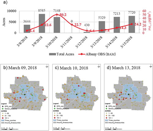
We focus our analysis on the March 8–15, 2018 period, which includes the National Ambient Air Quality Standard (NAAQS) exceedance for PM_2.5 (daily PM_2.5 concentration > 35 µg/m³) on March 10. The daily total burn area in the twelve counties surrounding the monitors on that day and the previous day are larger than 7,000 acres (Figure 2). Also, from March 13 to 15 (Figure 2d), the daily total burn area is larger than 5,000 acres each day. It is possible that those fires had a severe impact on air quality but the impact was missed in the observations by the BAM and the low-cost sensors. In order to evaluate the performance of low-cost sensors during the exceedance day and the feasibility of chemical transport models to capture the temporal and spatial variations of the fire impact, an eight-day period (March 08–15) was simulated using Weather Research and Forecasting (WRF) model version 3.6 (WRF Model V3.6 2019), a mesoscale numerical weather prediction model, and CMAQ version 5.0.2, which is equipped with DDM. The impacts of prescribed burning emissions on PM_2.5 are calculated by CMAQ-DDM as the first-order sensitivities of concentrations to those emissions. The model configurations are the same as in the HiRes2 air quality forecasting system (Huang et al. 2020; Odman et al. 2018). The prescribed burning emissions are calculated by using the BlueSky framework (Larkin et al. 2009) according to the burn area information from the Georgia Forestry Commission’s (GFC) burn permit database. The fuel map in BlueSky is from the Fuel Characteristic Classification System (FCCS) (McKenzie et al. 2007). The computer program Consume 3.0 (Joint Fire Science Program 2009) was used to calculate fuel consumption in BlueSky. All fires are assumed to start at 11:00 local time and last 3 hours. Other emission sources’ data were processed by Sparse Matrix Operator Kernel Emissions (SMOKE) (Carolina Environmental Program 2013) based on the 2011 National Emissions Inventory (NEI) (US EPA, 2019). The grid used by both WRF and CMAQ has a horizontal resolution of 4 km over Georgia and surrounding areas as the innermost nest of a grid system that has 36-km resolution over the contiguous US and 12-km resolution over the eastern US. It has 13 vertical layers starting with a 20-m height at the ground and expanding with altitude until approximately 20 km.

Figure 2. (a) Daily total burn area at the three low-cost sensor deployed (Dougherty, Lee, Worth) and nine surrounding counties according to the Georgia Forestry Commission (GFC) permit database and daily average PM_2.5 concentration from the BAM at Albany (red); Permitted burns at the three low-cost sensor deployed counties (blue) and nine surrounding counties (gray) on b) March 9, c) March 10 and d) March 13, 2018. Red circles represent fires larger than 150 acres, orange circles represent fires larger than 50 acres and smaller than 150 acres; yellow circles represent fires smaller than 50 acres; Green circles represent low-cost sensors and the black star represents the Albany EPD site

Data fusion

We applied a data fusion method that combines simulations from CMAQ-DDM at 4 km resolution and observations from both the BAM at Albany EPD site and low-cost sensors to generate hourly spatiotemporal fields for exposure estimates. The method has been used to estimate the daily PM_2.5 and its components and gaseous fields for Georgia (Friberg et al. 2016) and North Carolina (Huang et al. 2018a). Details of the method can be found in previous publications (Friberg et al. 2016; Huang et al. 2018a) and briefly summarized in the Supporting Information. The data fusion approach fuses the simulated fields with ground-level observations, so we expect to see strong agreement in the modeled grid cells that include an observation.

We also conducted a location-based data withholding evaluation. Observations from one location (Albany EPD site, DCHS or WCHS) were withheld and data fusion was performed with observations from the two remaining locations. The withheld observations for that iteration were compared with the data-fused simulated values to evaluate the performance of the data fusion method and assess whether low-cost sensors could provide extra spatial and temporal information to improve the accuracy of exposure fields.

Results and discussion

Comparison of observations from low-cost sensors and BAM

Comparison between low-cost sensors and BAM using different correction methods

Daily PM_2.5 observations from EPD’s BAM at the Albany site and collocated low-cost sensor show that the low-cost sensor captures the variations in the PM_2.5 levels (Figure S2). Daily PM_2.5 concentrations using RH correction match better with BAM observations, especially at the peak concentrations. Comparison between the observations from BAM at Albany EPD site and daily PM_2.5 measurements by the collocated low-cost sensor show that RH correction performs slightly better, with a higher R² and slope and lower intercept (Figure S3). Since RH correction results in better low-cost sensor performance, the following discussion will focus on results obtained using RH correction only.

Time series of PM_2.5 from low-cost sensors and BAM

Most of the hourly PM_2.5 concentration peaks detected by EPD’s BAM at the Albany site are captured by the low-cost sensors (Figure S4). However, low-cost sensors are less sensitive to changes in PM_2.5 concentrations than the BAM, and record less variation [standard deviation (SD) of ~5 µg/m³; Table 2] than that of the BAM at Albany EPD site (SD = 8.68 µg/m³). Differences in the observed peak levels between the BAM and the sensors other than at the Albany EPD site are likely due to the presence of small fire plumes, which can lead to a very heterogeneous PM_2.5 field on scales of less than 1 km. Sometimes the narrow fire plumes would miss some of the sensors completely. The Albany low-cost sensor observed elevated levels of PM_2.5 on May 7, 2018 (max of 36 µg/m³), though these were less than those observed by the BAM (max of 46 µg/m³) at Albany EPD site (Figure S5). On May 11, 2018, PM_2.5 levels above 20 µg/m³ were detected by the BAM. The Albany low-cost sensor also observed high concentrations during the same periods (8:00–11:00), but the peak hour from the Albany low-cost sensor (10:00) is two hours later than that from the BAM at 8:00 (Figure S5). The low-cost sensors at Albany EPD site and DCHS both capture a peak > 40 µg/m³ on April 26; however, there are no valid values on that day from the BAM. Low-cost sensors may thus serve as a supplement for regulatory monitors in such instances.

Table 2. Mean and standard deviation (SD) of hourly PM_2.5 concentrations from the BAM at the Georgia EPD monitoring site in Albany and low-cost sensors during their measurement periods (Table 1)

Hourly	Albany (BAM)	Albany	DCHS	LCHS	WCHS
Mean (µg/m^3)	7.98	7.50	6.69	6.10	6.86
SD (µg/m^3)	8.68	5.06	4.81	3.70	5.62

Daily trends of PM_2.5 concentrations from low-cost sensors and Albany EPD site show that the low-cost sensors did not capture levels as high as the BAM (Figure S6). On March 10, 2018, the BAM recorded 50 µg/m³, an exceedance of the 35 µg/m³ daily average PM_2.5 NAAQS, and the concentration of 36 µg/m³ from DCHS low-cost sensor, the closest low-cost sensor to the Albany EPD site, also detected the exceedance despite this value being 30% lower than the BAM. However, this value is still the highest value observed among the low-cost sensors during the measurement period (Figure S6). Note that the Albany low-cost sensor was not operational on that day.

Comparisons of hourly and daily PM_2.5 concentrations between low-cost sensors and BAM

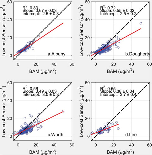
Figures S7 and Figure 3 demonstrate that low-cost sensors underestimate the PM_2.5 concentrations with respect to the BAM observations at EPD’s Albany monitoring site with linear regression slopes of less than 1. The low-cost sensor at the EPD site has the largest R² (= 0.83) among all four sensors. Note that this value is within the R² range reported by Sayahi, Butterfield, and Kelly (2019) for a similar sensor under comparable conditions. For the DCHS low-cost sensor, which is the second closest low-cost sensor to the monitoring site (1 km), the R² (= 0.72) and slope (= 0.55) of the linear regressions of daily PM_2.5 concentrations with the BAM observations at Albany EPD site (Figure 3b) are the largest among the three high school low-cost sensors. Lower R² values from comparisons with the LCHS and WCHS low-cost sensors do not mean those low-cost sensor performances are not adequate. With increasing distance between the low-cost sensors and EPD’s BAM at Albany monitoring site, measured concentrations are more likely to reflect impacts from different fire plumes; therefore, those lower R² values are expected. They show the spatial variation of fire impact on PM_2.5 concentrations and that a single monitoring site may miss high concentrations in the area.

Figure 3. Comparisons of daily PM_2.5 concentrations between low-cost sensors and the BAM at Georgia EPD site in Albany from May 16, 2017 to June 20, 2018: a) Albany sensor (no data before March 14, 2018); b) Dougherty Comprehensive High School (DCHS) sensor; c) Worth County High School (WCHS) sensor (no data from May 09, 2018 to June 20, 2018); d) Lee County High School (LCHS) sensor (no data from July 28, 2017 to March 13, 2018 and April 21, 2018 to June 20, 2018)

Both the hourly and daily PM_2.5 concentration regressions between the BAM and low-cost sensor at the Albany EPD site have slopes less than 1 (Figure 3a, S7a). In general, the observations of PM_2.5 concentrations from the low-cost sensor are higher than those from the BAM below 10 µg/m³ and lower for larger concentrations. The comparisons between the BAM and sensors at DCHS and WCHS with a cutoff at 95th percentile of BAM observations (Figure S8) shows that almost all the observations from DCHS and WCHS low-cost sensors are below the diagonal line.

Intercomparison between low-cost sensors

The R² values of linear regressions between low-cost sensors are around 0.9 and the slopes are very close to 1 (Figure S9). As the distance between the low-cost sensor at the Albany site and another sensor (DCHS, LCHS, or WCHS) increases, R² decreases. This is a direct result of the spatial variation in prescribed burning impact on PM_2.5 concentrations. While DCHS, which has the low-cost sensor closest to the Albany EPD site, has the highest R² (0.98), WCHS, the farthest low-cost sensor, has the lowest R² (0.90).

Air quality simulation results: PM_2.5 concentrations and fire contributions

The CMAQ simulations do not capture well the temporal variation of PM_2.5 concentrations detected by both BAM and low-cost sensors (Figure S10). The high PM_2.5 concentrations are mainly from fire impact (DDM results). The following discussion will focus on two periods: March 9–10 and March 13–14, 2018 to explain possible reasons why the simulations do not agree with observations.

On March 9, the simulation predicts the peak concentration to be around 85 µg/m³, which is in good agreement with the observed peak level, but the observed occurs five hours earlier (Figure 4). This mismatch in the time of occurrence may be due to inaccurate starting time and duration of the fires in the model. Recall all the fires in the CMAQ-DDM model were assumed to start at11:00 and last 3 hours in the simulation; however, permit records for March 9 show fires approved to start in the afternoon and end at night. However, the actual start time and duration of fires are not known since no post-burn information is available. Also, since there are hundreds of fires during highly active burn days, it is impossible to differentiate each fire and define a specific start and end time. On March 10, the observed PM_2.5 peak at 10:00 (Figure 4a) may be caused by a new fire starting early and located close to the monitoring site. However, the simulation does not have any fires starting before 11:00 and, since the boundary layer is changing rapidly at 10:00, it is hard to distinguish which fire causes the peak. The simulation does not capture the exceedance of the 35 µg/m³ daily PM_2.5 NAAQS standard either. The large difference between the observation and simulation at the beginning hours of March 10 may be mainly caused by simulated meteorology. The observed wind speed is zero from 1:00 to 6:00 and then again from 19:00 to 0:00; however, the WRF-simulated wind speed is larger than 2 m/s during the same periods (Figure 4c). A systematic bias that leads to overestimated nighttime wind speed have been reported in other applications of WRF (Garcia-Menendez, Hu, and Odman 2013; McNider et al. 2018).

Figure 4. Comparisons between hourly observed and simulated PM_2.5 concentrations, and the simulated fire impact on March 9–10, 2018 at a) Albany EPD site (BAM), and b) DCHS site (sensor); and c) Hourly wind speed observations at the Southwest Georgia Regional Airport (KABY) and simulations at KABY and Albany EPD site

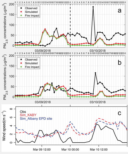
The DCHS low-cost sensor and EPD’s Albany site are located in two neighboring grid cells in the model simulations. At 18:00 on March 9, the simulated PM_2.5 concentrations at these two grid cells are almost the same (~ 30 µg/m³). However, the observations from EPD’s BAM at Albany (80 µg/m³) and low-cost sensor (50 µg/m³) at DCHS are quite different. The simulation does not capture this large spatial gradient in PM_2.5 concentrations (Figure 4(a,Figure 4b)). On a different note, the peak concentration at the Albany EPD site is observed at 10:00 on March 10 (Figure 4a), while the peak at DCHS occurs at 11:00 (Figure 4b). There may be fires or lingering smoke nearby impacting the low-cost sensors at DCHS.

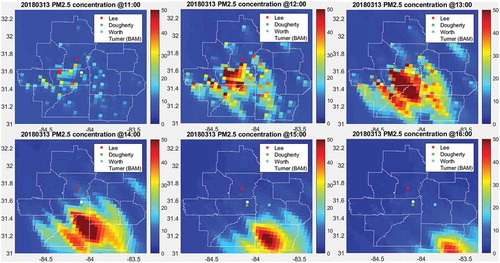
For the WCHS low-cost sensor, the peak at 13:00 (Figure S11) on March 13, 2018 is caused by medium size fires (51 to 150 acres) to the northwest, marked by the orange circles in Figure 2d. There are several large fires (> 150 acres) to the west and southwest; however, their smoke plumes move to the southeast under northwesterly winds and miss the Albany EPD site as well as the DCHS low-cost sensor (Figure 5). The observations at both locations are quite flat at low concentrations from 11:00 to 16:00 (Figure S11). Meanwhile, the counties to the south, including parts of Dougherty County, are severely affected by those large fires as shown in Figure 5, but there are no observations in this area to confirm this.

Figure 5. Spatial fields of hourly PM_2.5 concentrations on March 13 from 11:00 to 16:00: Georgia EPD site in Albany (white dot), DCHS (green dot), WCHS (blue dot) and LCHS (red dot)

Data fusion and data withholding results

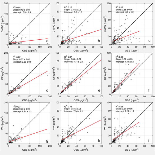
There is little correlation between observations and CMAQ simulations at EPD site in Albany, DCHS and WCHS (Figure 6a-c). Due to the nature of data fusion method (i.e., observation values dominate at the grid cell where the monitoring site is located), the strong correlations between observations and data fusion results (Figure 6d-f) are expected. The results of the data withholding evaluation show that low-cost sensors could improve the accuracy of exposure fields compared to raw CMAQ results, especially for the data withholding test at Albany EPD site (Figure 6g) that uses observations from two low-cost sensors located at DCHS (1 km away from the EPD site) and WCHS only. It shows an increased R² of 0.27 (Figure 6g) compared to 0.04 (Figure 6a) from CMAQ. The increase of R² is significant (from 0.17 to 0.38) even at WCHS where data from sites 25 km away are being fused. This evaluation shows that using low-cost sensors and applying the data fusion method could improve the accuracy of estimated exposure fields. Nevertheless, there is still a large fraction of the variability that needs to be explained.

Figure 6. Comparisons of hourly PM_2.5 observations at Albany EPD site (BAM), and at DCHS and WCHS sites (low-cost sensors) with PM_2.5 simulations from CMAQ (a, b, c), full data fusion (DF) (d, e, f), and DF with data withholding (WH) (g, h, i). The red lines are the linear regression trendlines

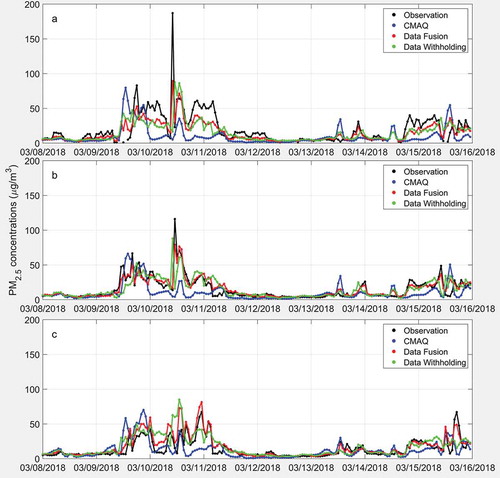
The temporal trends at the three locations (Figure 7) reflect similar trends that show how including observations from low-cost sensors can improve the accuracy of the final exposure fields. Using low-cost sensor observations could decrease the underestimation of prescribed burning impacts during the night time of model simulations, which is a systematic problem of the meteorological model with overestimation of the nighttime wind speed. Failure to predict the exceedance day on March 10 was mainly due to the night time underestimation of PM_2.5 concentrations. The data fusion as well as data withholding results at Albany EPD site agree better with the observations and capture the high level of PM_2.5 concentrations compared to CMAQ simulations (Figure 7). The early morning and nighttime results on March 10, March 11, March 14 and March 15 all show similar improvements. The missing peaks also have been adjusted to get closer to the observations by including observations from low-cost sensors. For example, the peak concentration on March 10 detected around 10:00at the Albany EPD site was missed by the CMAQ simulation; however, the data withholding result captures this peak, although with a delay of one hour (Figure 7a). The comparisons at DCHS and WCHS all show similar findings that early morning and midnight underestimations of PM_2.5 concentrations and missing peaks have been adjusted to be closer to observations.

Figure 7. Hourly PM_2.5 concentrations from observations (black lines), CMAQ simulations (blue lines), data fusion (red lines), and data fusion with data withholding (green lines) at a) Georgia EPD site in Albany, b) DCHS, and c) WCHS on March 8–16, 2018, EST

Conclusion

The sparsity of air quality monitors limits our ability to understand air pollution dynamics, evaluate air quality models, assess potential health impacts of air pollution and identify the most effective strategies to improve air quality and protect public health. The shortage of monitoring sites in Southwestern Georgia is of particular importance because of the widespread use of prescribed burning and its influence on local air quality and public health. As shown here, low-cost PM sensors can potentially be used to detect prescribed burning impacts and may provide additional spatial and temporal information that may be missed by model simulations. Further, they can provide supplemental information on air quality when regulatory monitors fail or when there is a lack of monitors in a given location. However, low-cost sensor collocation with regulatory monitors is important and still needs further investigation to answer questions such as which data correction method should be used. Collocation at a distant site with a different level and mixture of PM_2.5 may result in poor low-cost sensor performance. In our case, using an RH correction factor in a linear-regression equation with measurements from a reference instrument at a local site improved the accuracy of the sensor measurements. Lack of any mid-study correction check is a limitation of our study.

Because of the highly non-homogeneous distribution of PM_2.5 concentrations in Southwestern Georgia, particularly when fire plumes are present, spatial gradients cannot be captured even with a 4-km resolution model simulation. 1-km (or finer) resolution together with better knowledge of start and end times of the burns are needed to improve simulations. However, the accuracy of the fire impact simulation is highly dependent on accurate modeling of the meteorology. The systematic high bias of wind speed at nighttime in the WRF model makes it harder to capture the temporal variation and level of pollution. Uncertainties in wind speed and wind direction limit the accuracy of the simulations.

The application of a data fusion method that include observations from low-cost sensors can improve the accuracy of exposure fields for hourly PM_2.5 concentrations. Adding observations from low-cost sensors reduces the underestimation of nighttime PM_2.5 concentrations and reproduces the peaks that are missed by the simulations. Here, a limited number of sensors placed at convenient sites showed that there is room for improvement. We recommend fusing model simulations with observations from a well-designed, dense network of low-cost sensors for improved estimation of exposures to smoke from prescribed burning.

Acknowledgment

This publication’s contents are solely the responsibility of the grantees and do not necessarily represent the official views of the supporting agencies. Further, the US Government does not endorse the purchase of any commercial products or services mentioned in the publication. The authors thank Dr. Karoline Johnson Barkjohn of US EPA for assembling the sensors used in this study and everyone who helped them with the deployment of their sensors, in particular:

• Mr. Jeffrey Ross and Ms. Chelsea Cox of Dougherty Comprehensive High School

• Mr. Kevin Taylor and Mr. Jayme Jones of Lee County High School

• Ms. Melissa Edwards and Ms. Kim Perrin of Worth County High School

• Mr. Ernesto Rivera, Mr. Ken Buckley and Ms. DeAnna Oser of Georgia Department of Natural Resources, Environmental Protection Division

Supplementary material

Supplemental data for this article can be accessed on the publisher’s website.

Disclosure statement

No potential conflict of interest was reported by the author(s).

Additional information

Funding

This publication was made possible in part by funding from the Joint Fire Science Program grant number 16-1-08-1, National Science Foundation grant number 1751601 and NASA Applied Sciences Program grant numbers NNX16AQ29G and NNH16AD18I.

Notes on contributors

Ran Huang

Ran Huang received her Ph.D. in Environmental Engineering from Georgia Institute of Technology in 2019. Her research interests lie in air quality modeling, wildland fires and their impacts on air quality and public health. Currently, she is an Air Quality Engineer at Hangzhou AiMa Technologies, Hangzhou, China.

Raj Lal

Raj Lal is a post-doc at the University of Michigan who completed his Ph.D. at Georgia Institute of Technology.

Momei Qin

Momei Qin is currently at Jiangsu Key Laboratory of Atmospheric Environment Monitoring and Pollution Control, Collaborative Innovation Center of Atmospheric Environment and Equipment Technology, School of Environmental Science and Engineering, Nanjing University of Information Science & Technology, Nanjing, China. She was a post-doc at Georgia Institute of Technology.

Yongtao Hu

Yongtao Hu, Ph.D., is a Senior Research Scientist in the School of Civil and Environmental Engineering at Georgia Institute of Technology.

Armistead G. Russell

Armistead G. Russell is Howard T. Tellepsen Chair and Regents’ Professor in the School of Civil and Environmental Engineering at Georgia Institute of Technology. He conducts policy-relevant research in the air quality area with a focus on health effects of air pollution.

M. Talat Odman

M. Talat Odman is Principal Research Engineer in the School of Civil and Environmental Engineering at Georgia Institute of Technology. He has over 30 years of research experience in the areas of atmospheric chemistry, air pollution meteorology, and air quality modeling. Since 2008, a major focus of his research has been wildland fires and their air quality impacts. His current research interests include the management of prescribed burning for optimal ecological and air quality results.

Sadia Afrin

Sadia Afrin is a Ph.D. candidate in the Department of Civil, Construction, and Environmental Engineering at NC State University. Her research work focuses on atmospheric modeling and data analysis approaches to assess regional-scale air quality and health impacts from wildland fire smoke.

Fernando Garcia-Menendez

Fernando Garcia-Menendez is an Assistant Professor in the Department of Civil, Construction, and Environmental Engineering at North Carolina State University. His research focuses on computational modeling to explore air pollution, climate change, and environmental policy.

Susan M. O’Neill

Susan M. O’Neill is an Air Quality Scientist with the US Department of Agriculture Forest Service. Her research focuses on real-time and retrospective atmospheric modeling of wildland fire smoke, calculation of fire emissions, and use of remotely-sensed data for smoke and fire to support Land Managers and agencies/personnel doing smoke forecasting.

References

- Barkjohn, K. K., M. H. Bergin, C. Norris, J. J. Schauer, Y. Zhang, M. Black, M. Hu, and J. Zhang. 2020. Using low-cost sensors to quantify the effects of air filtration on indoor and personal exposure relevant PM2.5 concentrations in Beijing, China. Aerosol Air Qual. Res. 20 (2):297–313. AAGR Aerosol and Air Quality Research. doi:10.4209/aaqr.2018.11.0394.
- Brook, R. D., B. Franklin, W. Cascio, Y. Hong, G. Howard, M. Lipsett, R. Luepker, M. Mittleman, J. Samet, S. C. Smith, et al. 2004. Air pollution and cardiovascular disease. Circulation 109 (21):2655–71. http://circ.ahajournals.org/content/109/21/2655.
- Byun, D., and K. L. Schere. 2006. Review of the governing equations, computational algorithms, and other components of the models-3 Community Multiscale Air Quality (CMAQ) modeling system. Appl. Mech. Rev. 59 (2):51. American Society of Mechanical Engineers. doi:10.1115/1.2128636.
- Carolina Environmental Program. 2013. Sparse Matrix Operator Kernel Emissions Modeling System (SMOKE) use manual, edited. https://www.cmascenter.org/smoke/documentation/3.5.1/manual_smokev351.pdf.
- Cohen, A. J., M. Brauer, R. Burnett, H. R. Anderson, J. Frostad, K. Estep, K. Balakrishnan, B. Brunekreef, L. Dandona, R. Dandona, et al. 2017. Estimates and 25-year trends of the global burden of disease attributable to ambient air pollution: An analysis of data from the global burden of diseases study 2015. Lancet 389 (10082):1907–18. doi:10.1016/S0140-6736(17)30505-6.
- Cortez-Lugo, M., M. Ramírez-Aguilar, R. Pérez-Padilla, R. Sansores-Martínez, A. Ramírez-Venegas, and A. Barraza-Villarreal. 2015. Effect of personal exposure to PM2.5 on respiratory health in a mexican panel of patients with COPD. Int. J. Environ. Res. Public Health 12 (9):10635–47. doi:10.3390/ijerph120910635.
- Delp, W. W., and B. C. Singer. 2020. Wildfire smoke adjustment factors for low-cost and professional PM2.5 monitors with optical sensors. Sensors 20 (13):3683. doi:10.3390/s20133683.
- Dennekamp, M., and M. J. Abramson. 2011. The effects of bushfire smoke on respiratory health. Respirology 16 (2):198–209. Wiley/Blackwell (10.1111). doi:10.1111/j.1440-1843.2010.01868.x.
- EPA, U.S. 2017. 2017 National Emissions Inventory (NEI) data. Accessed February 6, 2021. https://www.epa.gov/air-emissions-inventories/2017-national-emissions-inventory-nei-data.
- EPD, DNR. 2018. 2018 ambient air monitoring plan. Georgia department of natural resources, environmental protection division, air protection branch. Accessed February 11, 2021. https://airgeorgia.org/docs/2018%20Ambient%20Air%20Monitoring%20Plan.pdf
- Fann, N., B. Alman, R. A. Broome, G. G. Morgan, F. H. Johnston, G. Pouliot, and A. G. Rappold. 2018. The health impacts and economic value of wildland fire episodes in the US: 2008-2012. Sci. Total Environ. 610 (January):802–09. doi:10.1016/j.scitotenv.2017.08.024.
- Friberg, M. D., X. Zhai, H. A. Holmes, H. H. Chang, M. J. Strickland, S. E. Sarnat, P. E. Tolbert, A. G. Russell, and J. A. Mulholland. 2016. Method for fusing observational data and chemical transport model simulations to estimate spatiotemporally resolved ambient air pollution. Environ. Sci. Technol. 50 (7):3695–705. American Chemical Society. doi:10.1021/acs.est.5b05134.
- Gao, M., J. Cao, and E. Seto. 2015. A distributed network of low-cost continuous reading sensors to measure spatiotemporal variations of PM2.5 in Xi’an, China. Environ. Pollut. 199 (April):56–65. Elsevier. doi:10.1016/J.ENVPOL.2015.01.013.
- Garcia-Menendez, F., Y. Hu, and M. T. Odman. 2013. Simulating smoke transport from wildland fires with a regional-scale air quality model: Sensitivity to uncertain wind fields. J. Geophys. Res. Atmos. 118 (12):6493–504. John Wiley & Sons, Ltd. doi:10.1002/jgrd.50524.
- Gupta, P., P. Doraiswamy, R. Levy, O. Pikelnaya, J. Maibach, B. Feenstra, A. Polidori, F. Kiros, and K. C. Mills. 2018. Impact of California fires on local and regional air quality: The role of a low-cost sensor network and satellite observations. GeoHealth, June. Wiley-Blackwell. doi:10.1029/2018GH000136.
- Haikerwal, A., M. Akram, A. Del Monaco, K. Smith, M. R. Sim, M. Meyer, A. M. Tonkin, M. J. Abramson, and M. Dennekamp. 2015. Impact of fine particulate matter (PM2.5) exposure during wildfires on cardiovascular health outcomes. J. Am. Heart Assoc. 4 (7):e001653. American Heart Association, Inc. doi:10.1161/JAHA.114.001653.
- Han, I., E. Symanski, and T. H. Stock. 2017. Feasibility of using low-cost portable particle monitors for measurement of fine and coarse particulate matter in urban ambient air. J. Air Waste Manage. Assoc. 67 (3):330–40. Taylor & Francis. doi:10.1080/10962247.2016.1241195.
- Holder, A. L., A. K. Mebust, L. A. Maghran, M. R. McGown, K. E. Stewart, D. M. Vallano, R. A. Elleman, and K. R. Baker. 2020. Field evaluation of low-cost particulate matter sensors for measuring wildfire smoke. Sensors 20 (17):4796. MDPI AG. doi:10.3390/s20174796.
- Huang, R., M. Qin, Y. Hu, A. G. Russell, and M. T. Odman. 2020. Apportioning prescribed fire impacts on PM2.5 among individual fires through dispersion modeling. Atmos. Environ. 223:117260. Pergamon, January. doi:10.1016/J.ATMOSENV.2020.117260.
- Huang, R., X. Zhai, C. E. Ivey, M. D. Friberg, X. Hu, Y. Liu, Q. Di, J. Schwartz, J. A. Mulholland, and A. G. Russell. 2018a. Air pollutant exposure field modeling using air quality model-data fusion methods and comparison with satellite AOD-derived fields: Application over North Carolina, USA. Air Qual. Atmos. Heal. 11 (1):11–22. Springer Netherlands. doi:10.1007/s11869-017-0511-y.
- Huang, R., X. Zhang, D. Chan, S. Kondragunta, A. G. Russell, and M. T. Odman. 2018b. Burned area comparisons between prescribed burning permits in Southeastern United States and two satellite-derived products. J. Geophys. Res. Atmos. 123 (9):4746–57. Wiley-Blackwell. doi:10.1029/2017JD028217.
- Johnson, K. K., M. H. Bergin, A. G. Russell, and G. S. W. Hagler. 2016. Using low cost sensors to measure ambient particulate matter concentrations and on-road emissions factors. Atmos. Meas. Tech. Discuss. February 1–22. doi:10.5194/amt-2015-331.
- Johnson, K. K., M. H. Bergin, A. G. Russell, and G. S. W. Hagler. 2018. Field test of several low-cost particulate matter sensors in high and low concentration urban environments. Aerosol Air Qual. Res 18 (3):565–78. doi:10.4209/aaqr.2017.10.0418.
- Joint Fire Science Program. 2009. Consume 3.0-A software tool for computing fuel consumption. https://www.firescience.gov/projects/98-1-9-06/supdocs/98-1-9-06_FSBrief55-Final.pdf.
- Kelleher, S., C. Quinn, D. Miller-Lionberg, and J. Volckens. 2018. A low-cost particulate matter (PM2.5) monitor for wildland fire smoke. Atmos. Meas. Tech. 11 (2):1087–97. doi:10.5194/amt-11-1087-2018.
- Kelly, K. E., J. Whitaker, A. Petty, C. Widmer, A. Dybwad, D. Sleeth, R. Martin, and A. Butterfield. 2017. Ambient and laboratory evaluation of a low-cost particulate matter sensor. Environ. Pollut. 221 (February):491–500. Elsevier. doi:10.1016/J.ENVPOL.2016.12.039.
- Lal, R. M., K. Das, Y. Fan, K. K. Barkjohn, N. Botchwey, A. Ramaswami, and A. G. Russell. 2020. Connecting air quality with emotional well-being and neighborhood infrastructure in a US city. Environ. Health Insights 14 (1):117863022091548. SAGE Publications Inc. doi:10.1177/1178630220915488.
- Landis, M. S., R. W. Long, J. Krug, M. Colon, R. Vanderpool, A. Habel, and S. P. Urbanski. 2021. The U.S. EPA Wildland fire sensor challenge: Performance and evaluation of solver submitted multi-pollutant sensor systems. Atmos. Environ. 247:118165. doi:10.1016/j.atmosenv.2020.118165.
- Larkin, N. K., S. M. O’Neill, R. Solomon, S. Raffuse, T. Strand, D. C. Sullivan, C. Krull, M. Rorig, J. Peterson, and S. A. Ferguson. 2009. The bluesky smoke modeling framework. Int. J. Wildl. Fire 18 (8):906. CSIRO PUBLISHING. doi:10.1071/WF07086.
- McKenzie, D., C. L. Raymond, L.-K. B. Kellogg, R. A. Norheim, A. G. Andreu, A. C. Bayard, K. E. Kopper, and E. Elman. 2007. Mapping fuels at multiple scales: Landscape application of the fuel characteristic classification systemthis article is one of a selection of papers published in the special forum on the fuel characteristic classification system. Can. J. For. Res. 37 (12):2421–37. doi:10.1139/X07-056.
- McNider, R. T., A. Pour-Biazar, K. Doty, A. White, Y. Wu, M. Qin, Y. Hu, T. Odman, P. Cleary, E. Knipping, et al. 2018. Examination of the physical atmosphere in the great lakes region and its potential impact on air quality - over-water stability and satellite assimilation. J. Appl. Meteorol. Climatol 57 (12):2789–816. JAMC-D-17-0355.1, August. doi:10.1175/JAMC-D-17-0355.1.
- Napelenok, S. L., D. S. Cohan, Y. Hu, and A. G. Russell. 2006. Decoupled direct 3D sensitivity analysis for particulate matter (DDM-3D/PM). Atmos. Environ. 40 (32):6112–21. doi:10.1016/j.atmosenv.2006.05.039.
- NICC. 2017. Wildland fire summary and statistics annual report 2017. Accessed February 6, 2021. https://www.predictiveservices.nifc.gov/intelligence/2017_statssumm/annual_report_2017.pdf.
- Odman, M. T., R. Huang, A. A. Pophale, R. D. Sakhpara, Y. Hu, A. G. Russell, and M. E. Chang. 2018. Forecasting the impacts of prescribed fires for dynamic air quality management. Atmosphere 9 (6):220. doi:10.3390/atmos9060220.
- Rappold, A. G., J. Reyes, G. Pouliot, W. E. Cascio, and D. Diaz-Sanchez. 2017. Community vulnerability to health impacts of wildland fire smoke exposure. Environ. Sci. Technol. 51 (12):6674–82. American Chemical Society. doi:10.1021/acs.est.6b06200.
- Reisen, F., C. P. (Mick) Meyer, L. McCaw, J. C. Powell, K. Tolhurst, M. D. Keywood, and J. L. Gras. 2011. Impact of smoke from biomass burning on air quality in rural communities in Southern Australia. Atmos. Environ. 45 (24):3944–53. Pergamon. doi:10.1016/J.ATMOSENV.2011.04.060.
- Sayahi, T., A. Butterfield, and K. E. Kelly. 2019. Long-term field evaluation of the plantower PMS low-cost particulate matter sensors. Environ. Pollut. 245:932–40. doi:10.1016/j.envpol.2018.11.065.
- Stanaway, J. D., A. Afshin, E. Gakidou, S. S. Lim, D. Abate, K. H. Abate, C. Abbafati, N. Abbasi, H. Abbastabar, F. Abd-Allah, et al. 2018. Global, regional, and national comparative risk assessment of 84 behavioural, environmental and occupational, and metabolic risks or clusters of risks for 195 countries and territories, 1990-2017: A systematic analysis for the global burden of disease stu. Lancet 392 (10159):1923–94. Lancet Publishing Group. doi:10.1016/S0140-6736(18)32225-6.
- US Census Bureau. 2015. 2010 American community survey 5-year estimates data profiles. Accessed April 18, 2021. https://data.census.gov.
- US EPA. 2019. 2011 National Emissions Inventory (NEI) data. Accessed June 8, 2019. https://www.epa.gov/air-emissions-inventories/2011-national-emissions-inventory-nei-data.
- Valdés, A., A. Zanobetti, J. I. Halonen, L. Cifuentes, D. Morata, and J. Schwartz. 2012. Elemental concentrations of ambient particles and cause specific mortality in Santiago, Chile: A time series study. Environ. Heal. 11 (1):82. doi:10.1186/1476-069X-11-82.
- Van Den Heuvel, R., J. Staelens, G. Koppen, and G. Schoeters. 2018. Toxicity of urban PM10 and relation with tracers of biomass burning. Int. J. Environ. Res. Public Health 15 (2):320. doi:10.3390/ijerph15020320.
- West, J. J., A. Cohen, F. Dentener, B. Brunekreef, T. Zhu, B. Armstrong, M. L. Bell, M. Brauer, G. Carmichael, D. L. Costa, et al. 2016. What we breathe impacts our health: Improving understanding of the link between air pollution and health. Environ. Sci. Technol. 50 (10):4895–904. doi:10.1021/acs.est.5b03827.
- WRF Model V3.6. 2019. Accessed October 17, 2019. http://www2.mmm.ucar.edu/wrf/users/wrfv3.6/wrf_model.html.
- Zamora, M. L., F. Xiong, D. Gentner, B. Kerkez, J. Kohrman-Glaser, and K. Koehler. 2019. Field and laboratory evaluations of the low-cost plantower particulate matter sensor. Environ. Sci. Technol. 53 (2):838–49. American Chemical Society. doi:10.1021/acs.est.8b05174.
- Zhang, J., H. Sun, Q. Chen, J. Gu, Z. Ding, and Y. Xu. 2019. Effects of individual ozone exposure on lung function in the elderly: A cross-sectional study in China. Environ. Sci. Pollut. Res. 26 (12):11690–95. Springer Verlag. doi:10.1007/s11356-019-04324-w.
- Zheng, T., M. H. Bergin, K. K. Johnson, S. N. Tripathi, S. Shirodkar, M. S. Landis, R. Sutaria, and D. E. Carlson. 2018 April. Field evaluation of low-cost particulate matter sensors in high and low concentration environments. Atmos. Meas. Tech. Discuss. 1–40. doi:10.5194/amt-2018-111.