Ambient sampling of real-world residential wood combustion plumes

ABSTRACT

Wood smoke contains large quantities of carbonaceous aerosols known to increase climate forcing and be detrimental to human health. This paper reports the findings from our ambient sampling of fresh residential wood combustion (RWC) plumes in two heating seasons (2015–2016, 2016–2017) in Upstate New York. An Aethalometer (AE33) and a pDR-1500 were employed to monitor residential wood smoke plumes in Ithaca, NY through a hybrid mobile-stationary method. Fresh wood smoke plumes were captured and characterized at 13 different RWC sources in the city, all without significant influence from other combustion sources or atmospheric aging. Wood smoke absorption Ångström exponent (AAE) was estimated using both a one-component model, AAE_WB, and a two-component model, AAE_BrC (assuming AAE_BC = 1.0). Consistent with the recent laboratory studies, our results show that AAEs were highly variable for residential wood smoke for the same source and across different sources, with AAE_WB values ranging from 1.3 to 5.0 and AAE_BrC values ranging from 2.2 to 7.4. This finding challenges the use of using a single AAE wood smoke value within the range of 1 to 2.5 for source apportionment studies. Furthermore, the PM_2.5/BC ratio measured using optical instruments was demonstrated to be potentially useful to characterize burning conditions. Different wood smoke sources can be distinguished by their PM_2.5/BC ratio, which range between 15 and 150. This shows promise as an in-situ, cost-effective, ambient sampling-based method to characterize wood burning conditions.

Implications: There are two main implications from this paper. First, the large variability in wood smoke absorption Ångström exponent (AAE) values revealed from our real-world, ambient sampling of residential wood combustion plumes indicated that it is not appropriate to use a single AAE wood smoke value for source apportionment studies. Second, the PM2.5/BC ratio has been shown to serve as a promising in-situ, cost-effective, ambient sampling-based indicator to characterize wood burning conditions. This has the potential to greatly reduce the costs of insitu wood smoke surveillance.

Introduction

Residential wood combustion (RWC) has been increasingly adopted as an alternative to fossil fuel-heating in parts of Europe and the U.S., motivated by environmental and economic considerations. However, RWC has led to significant environmental and health impacts. The health effects of wood smoke are found to be comparable to those of fossil-fuel combustion sources (Naeher et al. 2007). According to the 2014 U.S. National Air Toxics Assessment (https://www.epa.gov/national-air-toxics-assessment), RWC is estimated to account for 36% of all non-point stationary source air-toxic cancer risks nationwide. A recent analysis indicates that biomass and wood are the leading sources of stationary source air pollution health impacts in 24 states across the U.S. (Buonocore et al. 2021). In New York State (NYS), RWC currently provides less than 2% of the overall residential heating market (NYSERDA 2016) but contributes to over 79% of primary PM_2.5 emissions from the residential sector, estimated by the 2017 U.S. National Emission Inventory (https://www.epa.gov/air-emissions-inventories/2017-national-emissions-inventory-nei-data). In fact, primary PM_2.5 emissions from RWC exceed those from the entire transportation sector in NYS. RWC contributes to not only regional air pollution, but also localized air pollution hotspots. Furthermore, excessive smoke from inefficient RWC devices often generates smoke nuisance complaints even in relatively less-populated areas.

Additionally, black carbon (BC) and brown carbon (BrC) aerosols emitted during biomass burning (including RWC) have been shown to cause climate forcing. BrC, more recently, has also been found to play an important role in light absorption (Saleh et al. 2013), especially in the UV range (Wang et al. 2016). Synergistically, these aerosol light absorption properties have been utilized to characterize the impact of biomass burning particulate matter (PM). The dependence of light absorption on wavelength is described by the absorption Ångström exponent (AAE) (Zhang et al. 2017). In source apportionment studies, the AAE values help identify the quantity of aerosols produced by either wood burning, fossil fuel combustion or biogenic emissions (Martinsson et al. 2017). In climate science studies, the AAE is an important parameter for modeling the effect of aerosols on Earth’s radiative balance (Pokhrel et al. 2016). However, the AAE from RWC aerosols is not a stable value over time. Atmospheric aging and photochemistry change the composition of the organic carbon aerosol (Jimenez et al. 2009) reducing the aerosol AAE. Values for wildfire aerosol AAE in the US have been found to be around 4 after several hours of atmospheric aging, but fall to around 1.5 after 50 hours (Healy et al. 2019). This has implications for using AAE in biomass burning source apportionment models. The AAE values reported here are all for very fresh ambient aerosol, typically no more than a few minutes old in dark wintertime conditions, and would typically represent an upper bound for AAE from RWC aerosols in ambient air.

A general assumption in source apportionment studies is that AAE for wood smoke falls in the approximate range from 1 to 2.5 (Grange et al. 2020; Martinsson et al. 2017; Titos et al. 2017) and a single AAE wood smoke value is chosen within this range to separate biomass burning PM from traffic-generated PM. However, studies have shown that the absorption properties measured for aerosols emitted during biomass burning are influenced by the type of fuel (Garg et al. 2016,) burning conditions of the fuel (Wang et al. 2020) and aging in the atmosphere (Kleinman et al. 2020; Pratap et al. 2019). As AAE is a crucial input for characterizing and mitigating PM pollution, it is necessary to have a robust understanding of wood burning AAEs in real-world conditions. This paper reports the findings from our ambient sampling of fresh RWC plumes in two heating seasons in Upstate New York. There are two main objectives in our study. First, we quantify the real-world AAE values from fresh RWC plumes compared with those adopted in source apportionment studies and derived from laboratory experiments. Second, we aim to develop an in-situ, cost-effective, ambient sampling-based method to characterize the wood burning conditions. Such a method can greatly equip local communities in enforcing and responding to wood smoke pollution, which in turns reduces RWC emissions and related human exposure.

This paper is organized as follows. First, we describe our methodology for gathering and processing real-world wood smoke data. Then we show the variability of fresh wood burning AAE values and discuss the promise of PM_2.5/BC for characterizing burning conditions. Finally, we conclude by providing a more nuanced understanding of real-world AAE and suggest further investigation of PM_2.5/BC.

Methodology

Field measurements

A hybrid mobile-stationary technique was adopted to collect residential wood smoke data in Ithaca, NY. The city is located in central New York State and has a population around 30,000. Field measurements took place in Winter 2015–2016 and Winter 2016–2017, primarily during the evenings. During this time, traffic was very low on the road and RWC was the dominant local PM emission source. Many neighborhoods in Ithaca are densely populated so RWC may cause localized air pollution hotspots. Our field measurements sought to capture these hotspots.

The sampling apparatus has been reported previously (Zhang et al. 2017) and only a brief description is provided here. Two fast-responding instruments, a personal DataRAM^TM Aerosol Monitor (Model pDR1500, Thermo Fisher Scientific, USA) and a seven-wavelength Aethalometer^TM (370 nm, 470 nm, 520 nm, 590 nm, 660 nm, 880 nm, and 950 nm; Model AE33, Magee Scientific, USA) were employed to capture individual wood smoke plumes, both being operated at a 1s time resolution. The AE33 was operated with T60 (Magee 8020) filter tape during Winter 2015–2016, but was switched to T×40 (Magee 8040) filter tape during Winter 2016–2017 due to manufacturer issues. The sampling inlets of both pDR-1500 and AE33, equipped with 2.5 µm sharpcut cyclones (BGI SCC 1.197 cyclone at 2.3 L min-1 for pDR-1500; BGI SCC 1.829 cyclone at 5 L min-1 for AE33), were mounted one foot above the sunroof of a hybrid electric vehicle (HEV). Although the AE33 employs automated real-time loading compensation, it is not appropriate for mobile monitoring where different combustion sources are sampled in rapid succession. Rather, we used the uncompensated channel data and manually advanced the tape whenever the readings from “Sen1Ch1” dropped more than one-third from the initial clean spot value. In doing so, filter loading was kept relatively low (370 nm ATN less than 40) to minimize any loading effects. By not using corrected data and keeping filter loading low, differences between the T60 filter tape and T×40 filter tape were also minimized. A flow-through type CO₂ probe (Model CARBOCAP GMP343, Vaisala, Woburn, MA), being operated at a 2s time resolution, was connected to the outlet of the AE33 to record the CO₂ levels. The pDR-1500 operated without RH correction. RH in the pDR-1500 sensing chamber was always less than 35% without additional sample heating as the instrument was inside a heated vehicle and the chamber temperature was well above the ambient dew point. The pDR-1500 was zeroed prior to each mobile run. The monitoring routes were recorded at 1s intervals from a Delorme BU-353S4 GPS receiver using Delorme Street Atlas 2015 PLUS Software.

All instruments were powered primarily by the HEV battery without self-pollution. The internal combustion engine of the HEV occasionally turned on to recharge the battery and caused brief periods of self-pollution. We recorded those conditions, generally characterized by both high CO₂ and low PM_2.5 levels, and removed them from subsequent data analysis.

The mobile monitoring occurred periodically from December 2015 to March 2016, and then from December 2016 to March 2017. Field measurements were conducted on days when the New York State Department of Environmental Conservation (NYSDEC) forecasted low temperatures and low wind speeds. On these days the local air quality impact from wood smoke was expected to be significant. We made a total of 38 data gathering trips (two in December 2015, seven in January 2016, five in February 2016, six in March 2016, eight in January 2017, seven in February 2017 and three in March 2017).

The early part of the 2015–2016 field campaign was dedicated to surveying general air quality levels in the Ithaca area and identifying a number of recurring hotspots. The rest of the 2015–2016 campaign and most of the 2016–2017 campaign focused on the recurring hotspots. In total, 13 different hotspots were identified. These hotspots are referred to as sources in the paper. The HEV was parked right outside the property lines of residential wood smoke sources in the downwind direction, which was determined by visual observation of the plume. This hybrid mobile-stationary monitoring technique allows for data collection from multiple sources as well as data collection from the same source on multiple days.

Plume identification

Two criteria were used to distinguish wood smoke plume data gathered near a wood smoke source from extraneous ambient data gathered, for example, while the car is driving. The first uses only AE33 measurements. The AE33 samples air through a spot on a filter tape. The instrument measures transmission of light through the spot on the filter at seven optical wavelengths as described in Section 2.1 and reports measurements as black carbon concentrations, BC(λ), in units of μg m⁻³ for each wavelength. Previous wood smoke studies and analysis of the 2015–2016 data suggest that elevated DC, also referred to as Delta C and defined as BC(370 nm)-BC(880 nm), is a good indicator of wood smoke plumes (Allen, Babich, and Poirot 2004; Wang et al. 2012; Zhang et al. 2017). Based on prior experience, DC values greater than 1.5 µg m⁻³ are indicative of ambient wood smoke plumes in Ithaca, NY and a threshold DC value of 1.5 µg m⁻³ was used to distinguish wood smoke plumes from ambient data.

The second criterion uses both AE33 and pDR1500 instruments. Wood smoke plumes should result in simultaneous elevated DC from the AE33 and elevated PM_2.5 from the pDR1500. However, the screening of raw data indicated a time offset between the DC and PM_2.5 values. This time offset varied among different data collection trips but remained constant within the same trip. The offset was always within 10 seconds. This implies that differing tubing setup, flow rates and instrument response times between the AE33 and pDR-1500 were main causes of the offset. Figure 1 illustrates an example on 30 January 2017 showing the offset between raw DC and raw PM_2.5 data. This offset is corrected by shifting DC to better align with PM_2.5. The time offset for this example is 6 seconds. As a necessary procedure, we shifted the raw DC data to synchronize the spikes of DC and PM_2.5 for all the trips.

Figure 1. Time-Aligning the DC and PM_2.5 data.

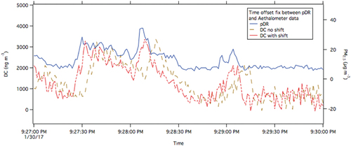
These methods identified wood smoke plumes that last between a few seconds and up to about a few minutes. The start and end of a plume are identified when DC values cross the 1.5 µg m-3 threshold, with data between the start and end of a plume maintaining DC values above the 1.5 µg m-3 threshold. After the start and end of a plume are determined, the 1s interval AE33 data is averaged over the duration of the plume to smooth the data and return one reading between the start and end of the plume event. As the time averaged data is used for a plume, effects such as time offset or noise are minimized.

Absorption ångström exponent (AAE)

The AE33 analyzes aerosols by measuring the transmission of light through sampled aerosol particles at seven different wavelengths. It reports the absorption as black carbon concentrations, BC(λ), in units of μg m⁻³ for each wavelength. BC(λ) can be converted to an absorption coefficient, b_abs (λ), by multiplying by the mass absorption coefficient, σ(λ), as shown in Equation (1)(1) $\mathrm{B}\mathrm{C}\left(\lambda \right)={\mathrm{b}}_{\mathrm{a}\mathrm{b}\mathrm{s}}\left(\lambda \right)/\sigma \left(\lambda \right)$(1) :

(1) $\mathrm{B}\mathrm{C}\left(\lambda \right)={\mathrm{b}}_{\mathrm{a}\mathrm{b}\mathrm{s}}\left(\lambda \right)/\sigma \left(\lambda \right)$(1)

Light absorption at different wavelengths is attributed to AAE_WB (WB for wood burning) (Favez et al. 2009; Grange et al. 2020; Martinsson et al. 2017; Sandradewi et al. 2008). AAE_WB can be approximated by fitting Equation (2)(2) ${\mathrm{b}}_{\mathrm{a}\mathrm{b}\mathrm{s}}\left(\lambda \right)=\mathrm{C}\cdot {\lambda }^{-\mathrm{A}\mathrm{A}\mathrm{E}\mathrm{\_}\mathrm{W}\mathrm{B}}$(2) to the seven-wavelength data points using a fitting coefficient, C. Because this method outputs a single AAE_WB for wood smoke, it is referred to as the one-component model:

(2) ${\mathrm{b}}_{\mathrm{a}\mathrm{b}\mathrm{s}}\left(\lambda \right)=\mathrm{C}\cdot {\lambda }^{-\mathrm{A}\mathrm{A}\mathrm{E}\mathrm{\_}\mathrm{W}\mathrm{B}}$(2)

Adapted from Chow et al. (2018), we also employed a two-component model which assumes that wood smoke light absorption can be attributed to two components, BC and BrC. The two-component model shown in Equation (3)(3) ${\mathrm{b}}_{\mathrm{a}\mathrm{b}\mathrm{s}}\left(\lambda \right)={\mathrm{q}}_{\mathrm{B}\mathrm{C}}\cdot {\lambda }^{-\mathrm{A}\mathrm{A}\mathrm{E}\mathrm{\_}\mathrm{B}\mathrm{C}}+{\mathrm{q}}_{\mathrm{B}\mathrm{r}\mathrm{C}}\cdot {\lambda }^{-\mathrm{A}\mathrm{A}\mathrm{E}\mathrm{\_}\mathrm{B}\mathrm{r}\mathrm{C}}$(3) has AAE_BC with a fitting coefficient q_BC to model BC light absorption, and AAE_BrC with another fitting coefficient q_BrC to represent BrC light absorption. AAE_BC is widely accepted to be around 1.0 (Kirchstetter, Novakov, and Hobbs 2004).

(3) ${\mathrm{b}}_{\mathrm{a}\mathrm{b}\mathrm{s}}\left(\lambda \right)={\mathrm{q}}_{\mathrm{B}\mathrm{C}}\cdot {\lambda }^{-\mathrm{A}\mathrm{A}\mathrm{E}\mathrm{\_}\mathrm{B}\mathrm{C}}+{\mathrm{q}}_{\mathrm{B}\mathrm{r}\mathrm{C}}\cdot {\lambda }^{-\mathrm{A}\mathrm{A}\mathrm{E}\mathrm{\_}\mathrm{B}\mathrm{r}\mathrm{C}}$(3)

The mass absorption coefficient, σ(λ) can be calculated from σ(880 nm) as shown in Equation (4)(4) $\sigma \left(\lambda \right)=\sigma (880\mathrm{n}\mathrm{m})\cdot (\lambda /880\mathrm{n}\mathrm{m}{)}^{-\mathrm{A}\mathrm{A}\mathrm{E}\mathrm{\_}\mathrm{B}\mathrm{C}}$(4) :

(4) $\sigma \left(\lambda \right)=\sigma (880\mathrm{n}\mathrm{m})\cdot (\lambda /880\mathrm{n}\mathrm{m}{)}^{-\mathrm{A}\mathrm{A}\mathrm{E}\mathrm{\_}\mathrm{B}\mathrm{C}}$(4)

Assuming AAE_BC = 1.0, BC(λ) can be expressed as shown in Equation (5)(5) $\mathrm{B}\mathrm{C}\left(\lambda \right)={\mathrm{b}}_{\mathrm{a}\mathrm{b}\mathrm{s}}\left(\lambda \right)/\sigma \left(880\mathrm{n}\mathrm{m}\right)\cdot \lambda /880\mathrm{n}\mathrm{m}$(5) :

(5) $\mathrm{B}\mathrm{C}\left(\lambda \right)={\mathrm{b}}_{\mathrm{a}\mathrm{b}\mathrm{s}}\left(\lambda \right)/\sigma \left(880\mathrm{n}\mathrm{m}\right)\cdot \lambda /880\mathrm{n}\mathrm{m}$(5)

Combining Equations (2)(2) ${\mathrm{b}}_{\mathrm{a}\mathrm{b}\mathrm{s}}\left(\lambda \right)=\mathrm{C}\cdot {\lambda }^{-\mathrm{A}\mathrm{A}\mathrm{E}\mathrm{\_}\mathrm{W}\mathrm{B}}$(2) and (5(5) $\mathrm{B}\mathrm{C}\left(\lambda \right)={\mathrm{b}}_{\mathrm{a}\mathrm{b}\mathrm{s}}\left(\lambda \right)/\sigma \left(880\mathrm{n}\mathrm{m}\right)\cdot \lambda /880\mathrm{n}\mathrm{m}$(5) ) results in Equation (6)(6) $\mathrm{B}\mathrm{C}\left(\lambda \right)={\mathrm{C}}^{\prime }\cdot {\lambda }^{\left(1-\mathrm{A}\mathrm{A}\mathrm{E}\mathrm{\_}\mathrm{W}\mathrm{B}\right)}$(6) where C’ = C/σ(880 nm) · 1/880 nm:

(6) $\mathrm{B}\mathrm{C}\left(\lambda \right)={\mathrm{C}}^{\prime }\cdot {\lambda }^{\left(1-\mathrm{A}\mathrm{A}\mathrm{E}\mathrm{\_}\mathrm{W}\mathrm{B}\right)}$(6)

Similarly combining Equations (3)(3) ${\mathrm{b}}_{\mathrm{a}\mathrm{b}\mathrm{s}}\left(\lambda \right)={\mathrm{q}}_{\mathrm{B}\mathrm{C}}\cdot {\lambda }^{-\mathrm{A}\mathrm{A}\mathrm{E}\mathrm{\_}\mathrm{B}\mathrm{C}}+{\mathrm{q}}_{\mathrm{B}\mathrm{r}\mathrm{C}}\cdot {\lambda }^{-\mathrm{A}\mathrm{A}\mathrm{E}\mathrm{\_}\mathrm{B}\mathrm{r}\mathrm{C}}$(3) and (5(5) $\mathrm{B}\mathrm{C}\left(\lambda \right)={\mathrm{b}}_{\mathrm{a}\mathrm{b}\mathrm{s}}\left(\lambda \right)/\sigma \left(880\mathrm{n}\mathrm{m}\right)\cdot \lambda /880\mathrm{n}\mathrm{m}$(5) ) results in Equation (7)(7) $\mathrm{B}\mathrm{C}\left(\lambda \right)=\mathrm{q}{\prime }_{\mathrm{B}\mathrm{C}}+\mathrm{q}{\prime }_{\mathrm{B}\mathrm{r}\mathrm{C}}\cdot {\lambda }^{\left(1-\mathrm{A}\mathrm{A}\mathrm{E}\mathrm{\_}\mathrm{B}\mathrm{r}\mathrm{C}\right)}$(7) where q’_BC = q_BC/σ(880 nm) · 1/880 nm and q’_BrC = q_BrC/σ(880 nm) · 1/880 nm:

(7) $\mathrm{B}\mathrm{C}\left(\lambda \right)=\mathrm{q}{\prime }_{\mathrm{B}\mathrm{C}}+\mathrm{q}{\prime }_{\mathrm{B}\mathrm{r}\mathrm{C}}\cdot {\lambda }^{\left(1-\mathrm{A}\mathrm{A}\mathrm{E}\mathrm{\_}\mathrm{B}\mathrm{r}\mathrm{C}\right)}$(7)

Both AAE_WB and AAE_BrC can be estimated by fitting data points from all seven wavelengths in the AE33, while C’, q’_BC and q’_BrC are fitting constants (different from q_BC and q_BrC in Equation (2)(2) ${\mathrm{b}}_{\mathrm{a}\mathrm{b}\mathrm{s}}\left(\lambda \right)=\mathrm{C}\cdot {\lambda }^{-\mathrm{A}\mathrm{A}\mathrm{E}\mathrm{\_}\mathrm{W}\mathrm{B}}$(2) ). Data was processed with Python and the curve_fit function from the SciPy library was used to perform the fitting (www.scipy.org). The fitting resulted in R² values predominantly above 0.98. Fit data with R² values below 0.9 were discarded, but this affected less than 1% of measured plumes. Figure S1 in the Supplemental Materials shows examples of the time averaged AE33 data for wood smoke plumes and corresponding model fits.

PM2.5/BC ratio

With synchronized AE33 and pDR-1500 plume data, we calculated the ratio of PM_2.5 concentration to BC concentration. The data obtained from the AE33 channel 6, BC6 or BC(880 nm), is the standard for reporting BC concentration. Each time an AAE is calculated for a wood smoke plume, a PM_2.5/BC ratio is also calculated. The PM_2.5/BC ratio is referred to as PM_2.5/BC in the remainder of this paper.

Results and discussion

AAE distributions from real-world RWC plumes

As mentioned in Section 2.1, wood smoke plumes were measured at 13 distinct sources. In total, over 300 distinct plumes were identified and AAE_WB and AAE_BrC values were calculated for each plume. There was variation in the duration of plumes measured, with a minimum plume duration of 5 seconds, an average duration of 21 seconds, and a maximum duration of 254 seconds. Figure (2) displays the AAE_WB and AAE_BrC calculated from all the sources. It is clear that fresh, real world AAE_WB and AAE_BrC values range greatly. As expected, the AAE_BrC values tend to be greater than the AAE_WB values.

Figure 2. Aae_brc and AAE_WB from RWC sources, including over 300 distinct plumes sampled in two heating seasons.

As shown in Figure 2, the observed AAE_WB distribution has a median of 3.3 and the standard deviation is 0.68. The greatest AAE_WB value calculated is 5.0 and the lowest calculated is 1.3. The observed AAE_WB median value is slightly greater than commonly reported ranges for fresh AAE_WB identified through laboratory testing. Fresh woodsmoke from seven types of forest wood showed AAE_WB ranging from 0.9 to 2.2 (Day et al. 2006). Testing of fresh woodsmoke from burning wood pellets shows AAE_WB ranging from 1.6 to 2.0 (Olson et al. 2015). Aerosols emitted from fresh wood-burning in a modern masonry heater and a pellet boiler were found to have AAE_WB values ranging from 1.0 to 1.5 (Helin et al. 2021). The AAE_WB values observed in our real-world measurements more closely resemble those from the fresh residential wood smoke measurements reported by Thatcher et al. (2014) that range from 1.9 to 3.3.

Real-world AAE values vary from some published laboratory results likely due to different burning conditions or fuels. Popovicheva and Kozlov (2020) compared AAE_WB during different burning phases, finding AAE_WB values up to 4.4 during a smoldering phase, and AAE_WB typically around 1 for open flaming smoke. Real-world burning-conditions may be higher-emitting than idealized laboratory conditions. The data highlights that fresh AAE_WB, even before any aging, varies with many burning parameters, and one cannot assume a constant value.

The AAE_BrC distribution is wider and has a greater median value than the AAE_WB distribution, with a median of 5.1 and a standard deviation of 0.97. The greatest AAE_BrC value found is 7.4 and the lowest is 2.2. This wider range of values is consistent with ranges of AAE values observed for laboratory studies of BrC. Fresh BrC emissions from cookstove wood combustion was found to have AAE values ranging from 4.75 to 10.9 (Xie et al. 2018). Isolated BrC from wood pyrolysis was shown to have AAE values ranging from 6.1 to 6.8 (Li et al. 2020). Data gathered from wood chips burned under smoldering conditions using a wood grill stove show that the AAE for light absorbing organic carbon (OC), another term for BrC (Xie et al. 2018,) has an average value of 4.74 (Zhong and Jang 2014). Further, these results are consistent with residential wood smoke data measured outside houses in California that shows the AAE for OC ranging from 3.02 to 7.39 and averaging 5.0 (Kirchstetter and Thatcher 2012). An additional consideration for evaluating AAE values across studies is the different approaches adopted for determining AAE. Using different wavelengths and fitting methods has been shown to impact AAE values (Lack and Cappa 2010) and may account for some of the variation across reported values.

Figure 3 shows the AAE_BrC and AAE_WB distributions for each of the 13 RWC sources. Each location is given a unique name in this paper to indicate the street in Ithaca where the data was captured without revealing the exact source locations. Note that TIOGA16 and TIOGA17 refer to the same location (i.e., the same wood smoke source), but the data was gathered one year apart. For the following discussion in Section 3.2, they are treated as separate sources. Within each location, there is variability in measured AAE values. The AAE distribution gathered from a single source can have a range as wide as 4.5.

Figure 3. AAE_brc and AAE_WB distributions for each RWC source location. Sources are placed in descending order based on median AAE_BrC value.

The sources are ordered in Figure 3 based on descending median AAE_BrC values. This ordering helps contrast the AAE_BrC distributions from the AAE_WB distributions. It is clear that variability between sources is more evident in the AAE_BrC distributions than for AAE_WB distributions. The median AAE_BrC values among the sources range between about 4 to 7. In contrast, median AAE_WB values for all sources, except for one, fall between the range of about 3 to 4.

While the sources are ordered by descending median AAE_BrC values, this same ordering does not result in descending median AAE_WB values. This implies median AAE_BrC values and median AAE_WB values are not strongly correlated. However, sources with the widest AAE_BrC distributions (i.e., TIOGA16, TIOGA17, AURORA) also have the widest AAE_WB distributions, indicating that operating conditions affect both AAE_BrC and AAE_WB. Laboratory experiments have shown that using the same device with different burning conditions can result in biomass burning emissions with different absorption properties (Holder et al. 2019).

Although BC makes up a relatively smaller portion of wood smoke PM when compared to BrC, BC still plays a significant role in light absorption. This is evidenced by comparing AAE_WB and AAE_BrC distributions. AAE_WB shows the combined effects of BC and BrC on light absorption, while AAE_BrC only shows the effects of BrC on light absorption. If all absorption were caused by BrC, we would expect AAE_BrC and AAE_WB to have similar distributions. However, we observe notable differences between the distributions which implies that the mixing state of BC and BrC influence the AAE of wood burning PM, even for fresh emissions.

Further, the range of AAE values observed both across different sources and within the same source underscores that AAE for wood burning emissions can be highly variable. We do not recommend assuming a fixed AAE value for source apportionment efforts. More accurate results could be obtained by sampling ambient conditions to understand the AAE distribution for aerosols in a local area.

PM2.5/BC distribution

In addition to calculating AAE_BrC and AAE_WB, the PM_2.5 and BC concentrations were also analyzed for each wood smoke plume. Our analysis suggests that different sources can be distinguished from one another when PM_2.5 vs BC is plotted. These unique distributions were initially noticed while examining TIOGA16 and TIOGA17, which represent data collected from the same source, just one year apart and under very different burning conditions.

Data from TIOGA16 were collected during the Winter 2015–2016 campaign. Near the end of the 2015–2016 campaign, the homeowner (i.e., the owner of the wood stove) approached the research team for advice as neighbors frequently complained about emissions from the homeowner’s wood stove. Since homes in Ithaca are relatively close together, wood smoke plumes do not need to travel far to enter nearby properties. To address this concern, the research team worked with this homeowner on clean burning practices. In particular, the homeowner was advised to stop burning wet wood, which was often used in Winter 2015–2016, and to start with smaller pieces of wood at first to help the fire heat up quickly when starting up. The research team returned to the same site and gathered data labeled TIOGA17 in Winter 2016–2017. The homeowner self-reported successfully adopting clean burning techniques and improved relations with neighbors as the wood smoke became less noticeable.

Figure 4a illustrates the PM_2.5 vs BC distribution for TIOGA16 and TIOGA17. The TIOGA16 data, representing high-emitting conditions, generally have a steeper slope and higher PM_2.5 concentrations. In contrast, TIOGA17 data, representing low-emitting conditions, have a shallower slope. There is a cluster of data points running parallel to the x-axis and a few points showing elevated PM_2.5 concentrations.

Figure 4. (A) PM2.5 vs BC for TIOGA16 and TIOGA17. (b) the distribution of PM2.5/BC ratios. TIOGA16, prior to adopting clean burning techniques, shows greater PM2.5/BC values.

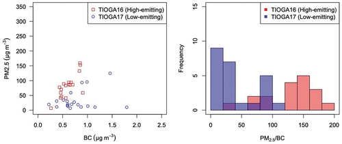
Figure 4b shows that the TIOGA16 PM_2.5/BC distribution is shifted to the right of the TIOGA17 PM_2.5/BC distribution. TIOGA16 has a mean PM_2.5/BC of 142.5, while TIOGA17 has a median PM_2.5/BC of 34.9.

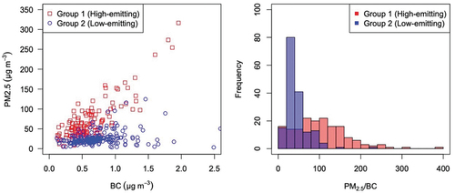
Based on the patterns seen in TIOGA16 and TIOGA17, the thirteen sources were placed into two groups. The groups were determined by visually comparing the PM_2.5/BC distribution for each source with the known high-emitting and low-emitting sources. Group 1 sources show distributions similar to the high-emitting conditions in TIOGA16. These include TIOGA16, LAKE, LOWER, BUFFALO, YATES. Group 2 sources show distributions similar to the low-emitting conditions in TIOGA17. These include TIOGA17, GILES, UPPER, HAN, SUN, HUDSON, COURT, AURORA. These groupings are intended to highlight the variety in burning conditions across sources rather than specifically defining the burning conditions of any particular source.

Figure 5a shows that Group 1 (high-emitting) and Group 2 (low-emitting) sources occupy different regions of the PM_2.5 vs BC plot. Figure 5b shows that the Group 2 PM_2.5/BC distribution is centered around 40. Almost all data from low-emitting Group 2 sources have PM_2.5/BC below 100. On the other hand, the PM_2.5/BC distribution for high-emitting Group 1 is centered around 100. Group 1 sources can frequently achieve PM_2.5/BC above 100.

Figure 5. (A) PM2.5 vs BC plots for Group 1, high-emitting sources, and Group 2, low-emitting sources. (b) the distribution of PM2.5/BC ratios. Group 1, high-emitting sources, show steep PM2.5/BC values.

It is promising to observe different burning conditions represented by different PM_2.5/BC distributions, which suggests that PM_2.5/BC could serve as a cost-effective metric for monitoring wood smoke emissions. For example, while collecting data from the LAKE source, the wood smoke plumes emitted from the chimney were very visible and dark in color and a strong burning odor was detectable even from inside the hybrid electric vehicle parked on the road. Later on when the data was processed, the PM_2.5/BC from LAKE was found to have a median value of 109.2, and frequently took on values between 100 and 200. This distribution is similar to that of the high-emitting TIOGA16 source so LAKE was categorized as Group 1. The PM_2.5/BC distribution for the LAKE source characterizes it as a high-emitting source of wood smoke, which is consistent with field observations.

Conclusion

Fresh ambient wood smoke emissions measured from 13 different sources in Ithaca were found to have a wide distribution of AAE values. The AAE_WB distribution ranged from 1.3 to 5.0 with a median of 3.3, higher than AAE_WB values from laboratory studies of fresh woodsmoke which fell between 0.9 to 2.2 (Day et al. 2006; Helin et al. 2021; Olson et al. 2015). However, the AAE_WB observed in our real-world measurements did resemble AAE_WB intentionally measured during different burning phases in laboratory studies, which ranged from 1.0 to 4.4 (Popovicheva and Kozlov 2020). The AAE_BrC distribution ranged from 2.2 to 7.4 with a median of 5.1. This range of values is similar to studies that found AAE for BrC of fresh wood smoke to fall between 3 and 10.9 (Kirchstetter and Thatcher 2012; Li et al. 2020; Xie et al. 2018; Zhong and Jang 2014).

AAE_WB and AAE_BrC for fresh ambient wood smoke were not observed as constant values. Wood smoke plumes measured from the same location, and on the same evening, were found to have a range of AAE values. The data highlights that fresh AAE, even before any aging, varies with many burning parameters. In particular, choosing a single AAE for wood burning emissions can cause source apportionment studies to incorrectly identify emission sources. This is problematic as accurate source apportionment is necessary to mitigate detrimental climate forcing and human health effects caused by wood burning emissions.

Additionally, PM_2.5 and BC measurements were also analyzed and the PM_2.5/BC ratio was found to be affected by burning conditions. Residential wood smoke emissions confirmed from high emitting sources had greater PM_2.5/BC ratios while low-emitting burning sources showed smaller PM_2.5/BC ratios. This introduces the prospect of assessing wood stove combustion conditions using widely available PM_2.5 and BC data. PM_2.5/BC distributions for a source are related to burning conditions based on experiences from one site where we observed different PM_2.5/BC distributions from high-emitting and low-emitting conditions. Based on this, the 13 sources were organized into two groups based on their distinguishable distributions of PM_2.5/BC values. One limitation of this study is the lack of data correlating the actual burning conditions for every source with PM_2.5/BC. Further investigation of the PM_2.5/BC is needed to examine its relationship with burning conditions and to understand if it is a viable and cost-effective monitoring measurement.

Acknowledgment

The authors acknowledge funding support from the New York State Energy Research and Development Authority (NYSERDA), and appreciate the assistance of Ye Lin Kim, Ye Xie and Qikun Wang at Cornell University with conducting the field measurements. The New York State Department of Environmental Conservation (NYSDEC) provided forecasting support for mobile measurements, and the authors thank Robert Gaza, John Kent and Julia Stuart for their kind assistance. The authors also thank Magee Scientific for loaning the Aethalometer Model AE33 employed in the field measurements and Dr. James Schwab from the Atmospheric Science Research Center at University at Albany for valuable assistance. AFL would like to acknowledge his support from the Engineering Learning Initiative (ELI) at Cornell University.

Disclosure statement

No potential conflict of interest was reported by the author(s).

Data availability statement

The data that support the findings of this study are available from the corresponding author, Dr. K. Max Zhang, upon reasonable request.

Supplementary material

Supplemental data for this paper can be accessed on the publisher’s website

Additional information

Funding

The work was supported by the New York State Energy Research and Development Authority [123059].

Notes on contributors

Alexander F. Li

Alexander F. Li completed his B.S. degree at Cornell University where he studied electrical and computer engineering and participated in environmental research. He earned a Master’s degree at Tsinghua University as a Schwarzman Scholar where he studied U.S.-China climate cooperation.

K. Max Zhang

K. Max Zhang is a professor of mechanical engineering at Cornell University, Ithaca, NY, USA.

George Allen

George Allen is the Chief Scientist at the Northeast States for Coordinated Air Use Management, Boston, MA, USA.

Shaojun Zhang

Shaojun Zhang was an Atkinson Postdoctoral Fellow at Cornell University. He is currently an assistant professor at School of Environment, Tsinghua University, China.

Bo Yang

Bo Yang was a postdoctoral researcher at Cornell University after receiving his PhD degree in mechanical engineering at the same institution. He is currently working at 3M.

Jiajun Gu

Jiajun Gu is currently a postdoctoral researcher at Cornell University after receiving her PhD degree in mechanical engineering at the same institution.

Khaled Hashad

Khaled Hashad received his PhD degree in mechanical engineering at Cornell University. He is currently working at Exponent, Inc.

Jeffrey Sward

Jeffery Sward received his PhD degree in mechanical engineering at Cornell University. He is currently working at Rocky Mountain Institute.

Dirk Felton

Dirk Felton is currently employed by the New York State Department of Environmental Conservation (NYSDEC) as a Research Scientist IV, where he oversees the air toxics monitoring program.

Oliver Rattigan

Oliver Rattigan is employed as a Research Scientist with the New York State Department of Environmental Conservation (NYSDEC) working on ambient air pollution monitoring.

References

- Allen, G.A., P. Babich, and R.L. Poirot 2004. Evaluation of a new approach for real time assessment of wood smoke PM. Air & Waste Management Association Visibility Specialty Conference on Regional and Global Perspectives on Haze: Causes, Consequences and Controversies, Asheville, NC, 1–11. https://www.nescaum.org/documents/2004-10-25-allen-realtime_woodsmoke_indicator_awma.pdf
- Buonocore, J.J., P. Salimifard, D.R. Michanowicz, and J.G. Allen. 2021. A decade of the U.S. energy mix transitioning away from coal: Historical reconstruction of the reductions in the public health burden of energy. Environ. Res. Lett. 16 (5):054030. doi:10.1088/1748-9326/abe74c.
- Chow, J.C., J.G. Watson, M.C. Green, X. Wang, L.W.A. Chen, D.L. Trimble, P.M. Cropper, S.D. Kohl, and S.B. Gronstal. 2018. Separation of brown carbon from black carbon for IMPROVE and chemical speciation network PM2.5 samples. J. Air Waste Manage. Assoc. 68 (5):494–510. doi:10.1080/10962247.2018.1426653.
- Day, D.E., J.L. Hand, C.M. Carrico, G. Engling, and W.C. Malm. 2006. Humidification factors from laboratory studies of fresh smoke from biomass fuels. J. Geophys. Res.: Atmos 111:D22. doi:10.1029/2006JD007221.
- Favez, O., H. Cachier, J. Sciare, R. Sarda-Esteve, and L. Martinon. 2009. Evidence for a significant contribution of wood burning aerosols to PM2.5 during the winter season in Paris, France. Atmos. Environ. 43 (22–23):3640–44. doi:10.1016/j.atmosenv.2009.04.035.
- Garg, S., B.P. Chandra, V. Sinha, R. Sarda-Esteve, V. Gros, and B. Sinha. 2016. Limitation of the use of the absorption angstrom exponent for source apportionment of equivalent black carbon: A case study from the North West Indo-Gangetic Plain. Environ. Sci. Technol. 50 (2):814–24. doi:10.1021/acs.est.5b03868.
- Grange, S.K., H. Lotscher, A. Fischer, L. Emmenegger, and C. Hueglin. 2020. Evaluation of equivalent black carbon source apportionment using observations from Switzerland between 2008 and 2018. Atmos. Meas. Tech. 13 (4):1867–85. doi:10.5194/amt-13-1867-2020.
- Healy, R.M., J.M. Wang, U. Sofowote, Y. Su, J. Debosz, M. Noble, A. Munoz, C.-H. Jeong, N. Hilker, G.J. Evans, et al. 2019. Black carbon in the lower fraser valley, British Columbia: Impact of 2017 wildfires on local air quality and aerosol optical properties. Atmos. Environ 217:116976. doi:10.1016/j.atmosenv.2019.116976.
- Helin, A., A. Virkkula, J. Backman, L. Pirjola, O. Sippula, P. Aakko‐saksa, S. Väätäinen, F. Mylläri, A. Järvinen, and M. Bloss. 2021. Variation of absorption ångström exponent in aerosols from different emission sources. J. Geophys. Res.: Atmos 126:e2020JD034094. doi:10.1029/2020JD034094.
- Holder, A.L., T.L.B. Yelverton, A.T. Brashear, and P.H. Kariher 2019. Black carbon emissions from residential wood combustion appliances; EPA/600/R-20/039, United States Environmental Protection Agency.
- Jimenez, J.L., M.R. Canagaratna, N.M. Donahue, A.S.H. Prevot, Q. Zhang, J.H. Kroll, P.F. DeCarlo, J.D. Allan, H. Coe, N.L. Ng, et al. 2009. Evolution of organic aerosols in the atmosphere. Science 326 (5959):1525–29. doi:10.1126/science.1180353.
- Kirchstetter, T.W., T. Novakov, and P.V. Hobbs. 2004. Evidence that the spectral dependence of light absorption by aerosols is affected by organic carbon. J. Geophys. Res. D: Atmos. 109 (21):1–12. doi:10.1029/2004JD004999.
- Kirchstetter, T.W., and T.L. Thatcher. 2012. Contribution of organic carbon to wood smoke particulate matter absorption of solar radiation. Atmos. Chem. Phys. 12 (14):6067–72. doi:10.5194/acp-12-6067-2012.
- Kleinman, L.I., A.J. Sedlacek, K. Adachi, P.R. Buseck, S. Collier, M.K. Dubey, A.L. Hodshire, E. Lewis, T.B. Onasch, J.R. Pierce, et al. 2020. Rapid evolution of aerosol particles and their optical properties downwind of wildfires in the western US. Atmos. Chem. Phys. 20 (21):13319–41. doi:10.5194/acp-20-13319-2020.
- Lack, D.A., and C.D. Cappa. 2010. Impact of brown and clear carbon on light absorption enhancement, single scatter albedo and absorption wavelength dependence of black carbon. Atmos. Chem. Phys. 10 (9):4207–20. doi:10.5194/acp-10-4207-2010.
- Li, X.H., M.D. Xiao, X.Z. Xu, J.C. Zhou, K.Q. Yang, Z.H. Wang, W.J. Zhang, P.K. Hopke, and W.X. Zhao. 2020. Light absorption properties of organic aerosol from wood pyrolysis: Measurement method comparison and radiative implications. Environ. Sci. Technol. 54 (12):7156–64. doi:10.1021/acs.est.0c01475.
- Martinsson, J., H.A. Azeem, M.K. Sporre, R. Bergstrom, E. Ahlberg, E. Ostrom, A. Kristensson, E. Swietlicki, and K.E. Stenstrom. 2017. Carbonaceous aerosol source apportionment using the Aethalometer model - evaluation by radiocarbon and levoglucosan analysis at a rural background site in southern Sweden. Atmos. Chem. Phys. 17 (6):4265–81. doi:10.5194/acp-17-4265-2017.
- Naeher, L.P., M. Brauer, M. Lipsett, J.T. Zelikoff, C.D. Simpson, J.Q. Koenig, and K.R. Smith. 2007. Woodsmoke health effects: A review. Inhal Toxicol 19 (1):67–106. doi:10.1080/08958370600985875.
- NYSERDA New York State Energy and Research Development Authority. 2016. New York State wood heat report: An energy, environmental, and market assessment, NYSERDA report 15-26, prepared by the Northeast states for coordinated air use management (NESCAUM), nyserda.ny.gov/publications.
- Olson, M.R., M.V. Garcia, M.A. Robinson, P. Van Rooy, M.A. Dietenberger, M. Bergin, and J.J. Schauer. 2015. Investigation of black and brown carbon multiple-wavelength-dependent light absorption from biomass and fossil fuel combustion source emissions. J. Geophys. Res.: Atmos. 120 (13):6682–97. doi:10.1002/2014JD022970.
- Pokhrel, R.P., N.L. Wagner, J.M. Langridge, D.A. Lack, T. Jayarathne, E.A. Stone, C.E. Stockwell, R.J. Yokelson, and S.M. Murphy. 2016. Parameterization of single-scattering albedo (SSA) and absorption angstrom exponent (AAE) with EC/OC for aerosol emissions from biomass burning. Atmos. Chem. Phys. 16 (15):9549–61. doi:10.5194/acp-16-9549-2016.
- Popovicheva, O., and V. Kozlov. 2020. Impact of combustion phase on scattering and spectral absorption of Siberian biomass burning: Studies in large aerosol chamber. Spie 11560:115604N. doi:10.1117/12.2575583.
- Pratap, V., Q.J. Bian, S.A. Kiran, P.K. Hopke, J.R. Pierce, and S. Nakao. 2019. Investigation of levoglucosan decay in wood smoke smog-chamber experiments: The importance of aerosol loading, temperature, and vapor wall losses in interpreting results. Atmos. Environ 199:224–32. doi:10.1016/j.atmosenv.2018.11.020.
- Saleh, R., C.J. Hennigan, G.R. McMeeking, W.K. Chuang, E.S. Robinson, H. Coe, N.M. Donahue, and A.L. Robinson. 2013. Absorptivity of brown carbon in fresh and photo-chemically aged biomass-burning emissions. Atmos. Chem. Phys. 13 (15):7683–93. doi:10.5194/acp-13-7683-2013.
- Sandradewi, J., A.S.H. Prévôt, S. Szidat, N. Perron, M.R. Alfarra, V.A. Lanz, E. Weingartner, and U.R.S. Baltensperger. 2008. Using aerosol light abosrption measurements for the quantitative determination of wood burning and traffic emission contribution to particulate matter. Environ. Sci. Technol. 42 (9):3316–23. doi:10.1021/es702253m.
- Thatcher, T.L., T.W. Kirchstetter, C.J. Malejan, and C.E. Ward. 2014. Infiltration of black carbon particles from residential woodsmoke into nearby homes. Open J. Air Pollut. 3 (4):111. doi:10.4236/ojap.2014.34011.
- Titos, G., A. Del Aguila, A. Cazorla, H. Lyamani, J.A. Casquero-Vera, C. Colombi, E. Cuccia, V. Gianelle, G. Mocnik, A. Alastuey, et al. 2017. Spatial and temporal variability of carbonaceous aerosols: Assessing the impact of biomass burning in the urban environment. Sci. Total Environ 578:613–25. doi:10.1016/j.scitotenv.2016.11.007.
- Wang, X., C.L. Heald, A.J. Sedlacek, S.S. de Sa, S.T. Martin, M.L. Alexander, T.B. Watson, A.C. Aiken, S.R. Springston, and P. Artaxo. 2016. Deriving brown carbon from multiwavelength absorption measurements: Method and application to AERONET and Aethalometer observations. Atmos. Chem. Phys. 16 (19):12733–52. doi:10.5194/acp-16-12733-2016.
- Wang, Y., P.K. Hopke, O.V. Rattigan, D.C. Chalupa, and M.J. Utell. 2012. Multiple-Year black carbon measurements and source apportionment using Delta-C in Rochester, New York. J. Air Waste Manage. Assoc. 62 (8):880–87. doi:10.1080/10962247.2012.671792.
- Wang, Y.J., M. Hu, N. Xu, Y.H. Qin, Z.J. Wu, L.W. Zeng, X.F. Huang, and L.Y. He. 2020. Chemical composition and light absorption of carbonaceous aerosols emitted from crop residue burning: Influence of combustion efficiency. Atmos. Chem. Phys. 20 (22):13721–34. doi:10.5194/acp-20-13721-2020.
- Xie, M.J., G.F. Shen, A.L. Holder, M.D. Hays, and J.J. Jetter. 2018. Light absorption of organic carbon emitted from burning wood, charcoal, and kerosene in household cookstoves. Environ. Pollut 240:60–67. doi:10.1016/j.envpol.2018.04.085.
- Zhang, K.M., G. Allen, B. Yang, G. Chen, J. Gu, J. Schwab, D. Felton, and O. Rattigan. 2017. Joint measurements of PM2.5 and light-absorptive PM in woodsmoke-dominated ambient and plume environments. Atmos. Chem. Phys. 17 (18):11441–52. doi:10.5194/acp-17-11441-2017.
- Zhong, M., and M. Jang. 2014. Dynamic light absorption of biomass-burning organic carbon photochemically aged under natural sunlight. Atmos. Chem. Phys. 14 (3):1517–25. doi:10.5194/acp-14-1517-2014.