Realistic operation of two residential cordwood-fired outdoor hydronic heater appliances—Part 2: Particle number and size

ABSTRACT

The use of wood as a fuel for home heating is a concern from an environmental health and safety perspective as biomass combustion appliances emit high concentrations of particulate matter. Wood burning significantly contributes to wintertime particulate matter concentrations in many states in the northern United States. Of particular concern are outdoor wood-fired hydronic heaters. These devices are concerning as they tend to have very large combustion chambers and typical use patterns can result in long periods of low output, which result in an increased particulate matter emission rate relative to high heat output operating conditions. In this study, the performance of two hydronic heaters operating under different combustion conditions, including four different heat output categories approximately corresponding to categories I–IV denoted in Environmental Protection Agency Method 28 Outdoor Wood-fired Hydronic Heaters, and during start-up and reloading events were investigated. Measurements of flue gas particulate number concentration and size for particles with aerodynamic diameters between 0.006 and 10 µm were made using a dilution sampling system. The measured particle number concentration in the flue gas was between 0.71 and 420 million particles per cubic centimeter and was dependent on fuel loading and heat output. For each hydronic heater tested, the highest average particle concentration was found at the beginning of each test during the cold-start condition. Additionally, the majority of the particles had aerodynamic diameters less than 0.100 µm (particles of this size made up between 64% and 97% of all particles) and less than 1% of all particles had aerodynamic diameters greater than 1 µm for all phases. For particles in the accumulation mode, between 0.100 and 1 µm, the mean particle diameter was dependent on fuel loading and heat output.

Implications: In this work, we provide information on the particle number concentration and particle size of emissions from outdoor cord- wood-fired hydronic heaters. Wood-fired hydronic heater data is sparsely available compared to wood stove data. Thus, additional data from this source help to inform the work of modelers and policy makers interested in hydronic heaters. The test method used in this work is also novel, as it is more inclusive of real-world use cases than the current certification method. Our data helps to validate the test method and allows for comparisons between real-world use case scenarios, and idealized test cases.

Introduction

The consumption of biomass for home space heating increased in the early 2000s in the United States, and especially so in the northeastern states (Berry 2014; NYSERDA 2016). According to the most recent American Housing Survey data between 2013 and 2019, the proportion of homes using wood for primary heating has stayed constant. Meanwhile, the proportion of homes using oil and natural gas for primary heating decreased and the proportion of homes using electricity increased (United States Census Bureau 2021). The primary pollutant associated with wood smoke is particulate matter (PM). Wood smoke contains PM of various compositions and sizes; ranging from large (>10 µm) brown carbon tarballs, to small (<10 nm) salt nuclei, and mixtures thereof (Kocbach Bølling et al. 2009; Trojanowski and Fthenakis 2019). Further, wood burning appliances emit a substantial portion of PM in many states in the US (NYSERDA 2008; Allen et al. 2011; Wang et al. 2012; Squizzato et al. 2019, Allen and Rector 2020, Ward and Lange, The impact of wood smoke on ambient PM2.5 in northern Rocky Mountain valley communities 2010; Ward et al. 2012, Kotchenruther 2016).

The literature on health effects indicates that exposure to wood smoke is likely to lead to increases in cardiovascular and respiratory symptoms, including myocardial infarction, decreased lung function, and exacerbation of prior conditions such as asthma and lung diseases and subsequent increases in emergency room visits and hospitalizations for these reasons (Kocbach Bølling et al. 2009; Naeher et al. 2007; Sehlstedt et al. 2010; Sigsgaard et al. 2015; U.S. EPA 2019; Weichenthal et al. 2017). Further, one study estimates that more than 30 million citizens in the United States could be impacted by wood smoke from in-home wood combustion (Noonan, Ward, and Semmens 2015). A study by Penn et al. estimated 10,000 premature mortalities per year in the U.S. from residential combustion. These deaths are driven primarily by health effects from PM_2.5 emissions, the majority of which is due to wood combustion (Penn et al. 2017). Therefore, it is clear that the increased use of biomass as a home heating fuel is a concern from an environmental health perspective.

Of particular concern are outdoor wood-fired hydronic heaters (HHs), as this particular appliance type has the highest emission factors for PM among other space heating appliance types. One study found that HH produces four times as much PM as conventional wood stoves, 12 times as much PM as Environmental Protection Agency (EPA) certified wood stoves, 1000 times as much PM as oil furnaces, and 1800 times as much PM as natural gas-fired furnaces (Schrieber et al. 2005) and other studies support this claim (NYSERDA 2012; U.S. EPA 1998, Rector, et al. 2017; Rector, Allen, and Johnson 2006). The reasons for the high emissions potential of HH are related to their function and design. Hydronic heaters are typically used for home heating via baseboard or traditional radiators. HH units are usually installed outdoors and have a water jacket, which captures the heat from combustion of the fuel. From there, the hot water is circulated indoors either through a heat exchange coil or directly to radiators. This purpose and general design lead to a large number of possible failure modes, leading to high PM emission.

For example, because home heating requires a constant source of energy, a HH unit must be able to provide heat continuously over a period of 12–24 hours. This result is typically achieved by including a large firebox in the design, which can be problematic as large fireboxes have wide gradients of oxygen and temperature, which can lead to high PM production zones/conditions within the firebox (Gibbs and Butcher 2010; Kinsey et al. 2012; U.S. EPA 1998). Heat demand is also highly variable both regionally and temporally (Ahmadi et al. 2020). This presents an issue for HH because unlike conventionally fueled boilers, which can reduce fuel input to meet the inconsistent need for heat, HH units operate as a batch process. This design element forces HH to rely on air flow controls to meet the demand. This presents a concern as the fuel in the unit must be constantly burning at a low output to meet baseline demand, and HH is notoriously polluting in this condition (U.S. EPA 1998; Gonçalves et al. 2011, Vicente, Duarte, et al. 2015b, Schmidl et al. 2011). This issue can be compounded by appliance owners who attempt to limit manual interaction with the hydronic heater by using large loads of fuel, which further aggravates the issue of inhomogeneous conditions within the firebox and stresses the appliance control system to provide extremely high air delivery rates (Johansson et al. 2004; Shen et al. 2013, Vicente, Duarte, et al. 2015a). The result in all cases is higher potential for emission of PM.

These concerns warrant further evaluation of HHs to inform homeowners, researchers, and policy makers regarding the magnitude of their pollutant capacity when used in the field. Given the conditions that raise the aforementioned concerns, special care must be taken in designing the test method to probe emissions during these same conditions. The current certification method, EPA Method 28 Outdoor Wood-fired Hydronic Heaters (United States Environmental Protection Agency 2017) has been criticized as being not representative of actual operation in homes (U.S. EPA 1998). This includes only steady-state combustion scenarios at <15%, 16–25%, 26–50%, and 100% rated heat output (United States Environmental Protection Agency 2017), the lowest of which can be optionally replaced. Research shows that high load steady state tests result in underestimates of emissions, as wood boilers operate most efficiently in that regime (Rector, et al. 2017). Additionally, the test method does not include any transient periods due to fuel loading, while some data suggest that transient conditions such as start-ups can have significantly increased PM emissions relative to steady-state combustion (Obernberger, Brunner, and Barnthaler 2007, Win and Persson 2014) (Win and Persson 2014).

This study investigated two HHs to assess the number concentration and size of the particulate emissions under different combustion conditions, including at load levels in the four different heat-output categories tested in EPA Method 28 Outdoor Wood-fired Hydronic Heaters and in transient combustion periods such as start-up, reloading, burnout, and during cyclic operation. The test method used during these experiments is “A Test Method for Certification of Cord Wood-Fired Hydronic Heating Appliances Based on a Load Profile: Measurement of Particulate Matter (PM) and Carbon Monoxide (CO) Emissions and Heating Efficiency of Wood-Fired Hydronic Heating Appliances,” n.d.” and is further described in Trojanowski et al. (Trojanowski, Lindberg et al. 2022).

Materials & Methods

This study includes data from triplicate testing of two HHs, denoted as hydronic heater A (HH A) and hydronic heater B (HH B), which were operated according to the load profile test method indicated above.

Appliances, fuel, and test method

The HHs investigated in this study were two similar appliances according to the manufacturer’s specifications and published EPA certification documents and are representative of the general population of HHs available for sale in the United States. Both HH appliances were modern units, which featured large internal water jackets, and sophisticated control systems based on feedback from internal sensors. HH A features an updraft, two-stage combustion system, where primary and secondary air were added to the fuel bed, followed by catalytic secondary combustion. HH B features a downdraft airflow pattern, and a two-stage gasification combustion system. The fuel used in each experiment was red oak cord wood. Red oak was chosen as the fuel due to its high heating value and low volatile content and because it is plentiful in the northeast, making it a common firewood in the area. The moisture content of the fuel used for these experiments was between 19% and 25% on average, as measured according to the method outlined in a study of the partial kiln drying and moisture measurement of cordwood for combustion by Dr. William Smith (Smith 2014).

The test method used during these experiments is explained in detail in “A Test Method for Certification of Cord Wood-Fired Hydronic Heating Appliances Based on a Load Profile: Measurement of Particulate Matter (PM) and Carbon Monoxide (CO) Emissions and Heating Efficiency of Wood-Fired Hydronic Heating Appliances,” n.d. The test protocol includes 10 distinct sections in which the HH is fueled three times, in order to test multiple permutations of fuel loading density and heat demand. A table including the order of the burn phases and a short description of each test section adapted from Trojanowski et al. (Trojanowski, Lindberg et al. 2022) is given in Table 1 and graphical representation of the heat demand and firebox loading density is shown in Figure 1.

Figure 1. Graph showing boiler output condition timeseries, fuel mass as red-dashed line, and boiler output as black-solid line.6.

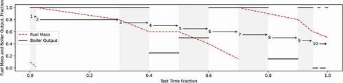
Table 1. Multi-phase testing protocol.

Phase	Description	Milestone to Signify End of Phase
Cold Start Fuel charge -kindling + starter fuel
1	Cold Start: Includes kindling (10% of fuel charge weight) made up of 50% small pieces and 50% larger kindling pieces	Once 80% of kindling fuel has been consumed
1^st fuel charge
2	Ramp-up to full load	Once 20% of 1^st fuel charge has been consumed during this phase
3	Maximum burn rate	Once 20% of 1^st fuel charge has been consumed during this phase
4	Steady state – less than 25% load	1.25 hours
5	Steady state – less than 50% load	Once 20% of 1^st fuel charge has been consumed
6	End phase – burn out	Once 85% of the 1^st fuel charge has been consumed, establishing a coal bed of 15% of the 1^st fuel charge
2^nd fuel charge
7	Reload – equivalent of a hot start	Only 10% of 2^nd fuel charge has been consumed during this phase
8	Steady state – less than 15% load	Greater of 2.0 hours or time required for 1 reheat firing cycles
9	Steady state 100% load	Only 20% of 2^nd fuel charge has been consumed during this phase
10	Cyclic operation (10 minutes off, 5 minutes on)	One the HH temperature has returned back to its starting point of temperature set-point reached
End of sampling		Let remainder of fuel burn out at maximum load – no sampling

The test phases are sequentially as follows: Phase 1 is a cold-start, where a small charge of fuel is loaded into the HH and combusted to establish a small char bed. Phase 2 is ramp-up, where a second fuel charge is added to the HH and combusted to bring the boiler to high-output steady-state operating temperatures and air-intake settings. Phases 3, 4, and 5 are category loads used in the current HH certification test, EPA Method 28 Outdoor Wood-fired Hydronic Heaters (United States Environmental Protection Agency 2017). Phase 3 is a high-output test section, where the HH is maintained at full output. Phase 4 is a medium-low output test section, where a heat demand of 16–25% of the appliance’s maximum rated output is applied to them. Phase 5 is a medium–high output period, where the HH’s heat output is set between 26% and 50% of the maximum output rate. Phase 6 is a burnout, where the remaining fuel is combusted at full output until only char remains. Phase 7 is a reload, where a large fuel charge (filling the chamber with as much fuel as possible) is added, and the HH returns to operating temperature. The intent of this section is to emulate users who fill the chamber with as much fuel as possible to avoid refueling their HH, which may occur overnight or during working hours. Phase 8 is a low output test section, where the HH’s heat output is reduced to <15% of the maximum, thus creating a scenario where smoldering of a large amount of fuel is likely to occur. Phase 9 is a second high output test section. Phase 10 tests cyclic operation; in this phase, the heat output is modulated between high and zero to emulate intermittent heat demand where once the load is satisfied, there is no longer a demand. For more detailed information on the appliance specifications, fuel preparation, and test method please refer to (Trojanowski et al. 2022) (Trojanowski, Lindberg et al. 2022).

Instrumentation

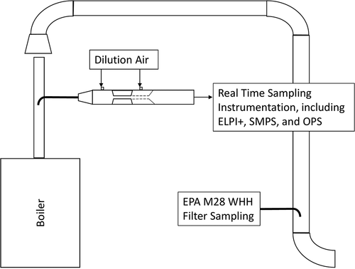
Measurements of particle concentration and size were made alongside thermal output, diagnostic measurements, and formal gravimetric PM emission rate measurements as the HHs operated according to the test method outlined in (Trojanowski et al. 2022) (Trojanowski, Lindberg et al. 2022). Appliance operational parameters such as fuel burn rate; flue gas, water, and internal temperatures; cooling water flow rates; and flue gas draft and composition were made alongside emission measurements. Particulate mass concentration and emission rates were measured according to the aforementioned test method, which calls for a dilution tunnel filter sampling technique. In addition, simultaneous measurements of flue gas particulate concentration, size, and character were made using a dilution sampling system. The schematic of the entire experimental setup is shown in Figure 2.

Figure 2. Schematic of combustion test set-up and location of various instrumentation.7.

In this article, only the size fractionated particle counter data collected using the dilution sampling system will be discussed. For additional information regarding gaseous pollutant emissions, HH operating parameters, and particle mass emission metrics please refer to Trojanowski et al. and for more information regarding measurements of optical particle measurements, such as black carbon concentration and angstrom absorption exponents please refer to Lindberg et al. (Trojanowski, Lindberg et al. 2022, 2022).

There are four primary components in Figure 2 related to particle number and size characterization. These are as follows: the dilution system and the three-size segregated particle counters, the Dekati Electrical Low-Pressure Impactor+ (ELPI+); the TSI Nanoscan Scanning Mobility Particle Sizer model 3910 (SMPS); and the TSI Optical Particle Sizer model 3330 (OPS).

The dilution system used for these experiments was a two-stage ejector dilutor with a heated sample inlet. During the experiments, a one standard liter per minute (SLPM) critical flow orifice was used to limit sampling flow rate to <1% of the stack gas by volume. The initial dilution ratio was set to 108:1 using the primary and secondary dilution air controls. The dilution ratio varied throughout each of the six experiments performed during the sampling campaign due to occlusion of the critical flow orifice. This effect was minimized by periodic testing of the dilution and sample gas flow rates and consequent replacement of the critical flow orifice when the dilution ratio had strayed noticeably from the initial value. The average dilution ratio during each of the six tests was 110 ± 22, 121 ± 30, and 109 ± 19 for the three tests of HH A and 210 ± 109, 133 ± 16, and 146 ± 60 for the three tests of HH B each, respectively. During data processing, the average dilution ratio for each respective experiment was applied to the measured particle counts across the test. By adding clean, dry dilution air, the relative humidity of the diluted aerosol sample was reduced below 25% and temperature to below 35°C during each experiment. The aerosol measurement instrumentation, including the ELPI+, SMPS, and OPS, was connected to the outlet of the dilution system, and excess diluted sample gas was directed from the overflow outlet outdoors. The ELPI+ is a size-resolved particle counter and gravimetric filter collection device capable of counting particles with aerodynamic diameters between 0.006 and 10 µm. The ELPI+ was operated according to manufacturer’s recommendations for all experiments including standard settings for flow rate (10 standard liters per minute (SLPM)), corona charger voltage (4500 kilovolts), current (1 microampere), and trap voltage (20 V). The impactor stages were loaded with 25 mm greased aluminum foil filters in all tests. The ELPI+ data was collected with 1 hertz (Hz) resolution and converted into 1 min averages during the data analysis step. It is notable that, in order to capture the entire runtime of the test method, the ELPI+ filters were not changed during the experiments. As a result, high mass loading of the filters occurred, which other groups suggest may skew the subsequent measurement of larger particles made by the ELPI+ (Maricq et al. 2007).

The SMPS is a size-resolved particle counter, which counts particles with mobility diameters between 0.010 and 0.420 µm separated into 13 size bins. The SMPS was operated in scanning mode during each experiment. The instrument settings were all set according to the manufacturer’s recommendation. These settings include an aerosol inlet flow rate of 0.75 SLPM and working fluid of 99.5+% pure spectroscopic-grade isopropyl alcohol. Utilizing scanning mode and a working fluid reservoir, 1-Hz size-segregated particle counts were collected continuously throughout each experiment.

The OPS is a size resolved optical particle counter, which counts particles with optical diameters between 0.300 and 10 µm into 17 bins. The OPS was operated according to the manufacturer’s recommendations with a flow rate of 1 SLPM with a set effective particle density of 1.0 g/cc and a refractive index of 1.2±0.0i. Other studies of biomass combustion aerosols have posited particle density and refractive index of wood smoke between 1.22–1.92 g/cc and 1.55–1.80 ± 0.01–0.50i, respectively (Levin et al. 2010). While the assumptions chosen here were outside the range found in the literature, presenting the data using the default assumptions is still valuable as a point for comparison to other studies. This is a particularly valid assumption given that the optical properties of woodsmoke are unique to each fuel, burn condition and appliance type, and combustion technique; it follows that optical properties also vary between appliances and phases of the operating protocol.

Data analysis

Each appliance was tested in triplicate according to the load profile test method described above. During each of the experiments, the size-resolved particle concentration in the flue gas was measured using multiple instruments spanning the size range of 0.006 to 10 µm. As the test progressed, the appliances reacted according to their control scheme to adjust combustion condition based on the heat demand and to changes in fuel load density as combustion progressed batchwise. These variables resulted in a dynamic aerosol concentration and Particle Size Distribution (PSD). In order to understand how the combustion process affected the aerosol concentration, the data was separated according to the phases outlined in the test method and the particle number concentration was analyzed to determine how the combustion conditions in each phase affected the aerosol concentration in the flue gas.

Particle number concentration data

Total particle number concentration was measured during each of the experiments. The ELPI+ is capable of counting particles between 0.006 and 10 µm, as such, total particle number concentration for all particles within that range will be written as PNC₁₀. Similarly, the SMPS is capable of counting particles between 0.010 and 0.420 µm and the OPS particles between 0.3 and 10 µm, and these particle concentrations are therefore denoted as PNC_.01-.420 and PNC_.3–10, respectively. All three instruments were used during each test with some minor exceptions due to instrument errors. This paper includes total particle number concentration results for only the ELPI+. The SMPS and OPS measurements supported the ELPI+ results and are provided in the Supplemental Information. The choice to feature the ELPI+ data was made simply because the measurement range of this instrument spans the widest range of particle sizes.

The mean one-minute average PNC₁₀ measurements for each phase of each triplicate test for both HHs are shown in Table 2. Figure 3 summarizes the PNC₁₀ data collected using the ELPI+ by HH and phase in the form of box-and-whisker plots.

Figure 3. Boxplot showing minute-by-minute total particle concentration as measured by the Electrical Low Pressure Impactor +. Red single-hatch is Hydronic Heater A, blue cross-hatch is Hydronic Heater B. Medians are shown as an Orange bar and means are shown as a green triangle. Notches extend to 95% confidence interval around median. Boxes extend to 25th and 75th percentile. Whiskers extend to the 5^th and 95^th percentiles. Mean is shown as green triangle, and outliers are shown as open circles.12.

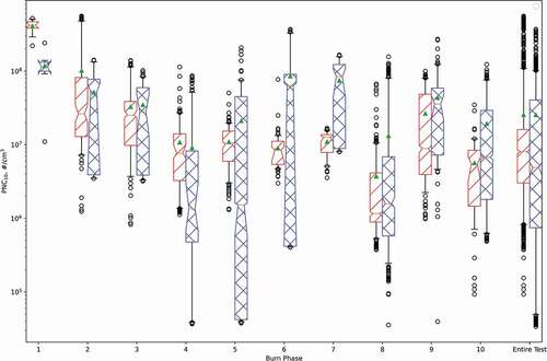
Table 2. Mean particle number concentration as measured using the Electrical Low-Pressure Impactor + instrument, in units of particle concentration per cubic centimeter (#/cm³), for each experimental test separated by appliance, test, and phase.

Test	Phase 1	Phase 2	Phase 3	Phase 4	Phase 5	Phase 6	Phase 7	Phase8	Phase 9	Phase 10	Entire Test	Weighted
1		1.1E+06	6.4E+06	4.1E+06	6.8E+06	6.2E+06	5.0E+07	9.9E+05	3.7E+06	7.1E+05	5.0E+06	4.8E+06
2	3.9E+08	1.3E+08	6.5E+07	1.6E+07	1.8e+07	1.2E+06	1.4E+07	8.2E+06	5.7E+07	6.4E+06	7.1E+07	6.4E+07
3	4.2E+08	1.5E+08	2.8E+07	9.9E+06	9.9E+06	7.8E+06	1.0E+07	2.2E+06	7.4E+06	5.6E+06	6.5E+07	6.2E+07
Average	4.0E+08	9.5E+07	3.3E+07	1.0E+07	1.2E+07	8.8E+06	9.7E+06	3.8E+06	2.3E+07	4.2E+06	4.9E+07	5.7E+07
Test	Phase 1	Phase 2	Phase 3	Phase 4	Phase 5	Phase 6	Phase 7	Phase 8	Phase 9	Phase 10	Entire Test	Weighted
1	4.8E+06	4.0E+06	3.6E+06	1.3E+06	1.4E+06	4.2E+05	8.5E+06	2.3E+06	6.2E+06	4.1E+06	3.6E+06	3.2E+07
2	1.2E+08	7.4E+07	6.1e+07	2.7E+07	5.6E+07	6.9E+07	1.4E+08	1.4E+07	3.8E+07	1.9E+07	6.2E+07	5.4E+07
3	1.1E+07	8.9E+07	3.0e+07	4.5E+04	5.7E+04	1.8E+08	9.3E+07	9.3E+07	7.4E+07	7.4E+07	6.4E+07	5.0E+07
Average	7.9E+07	5.6E+07	3.2E07	1.1E+07	1.9E+07	8.4E+07	7.9E+07	1.3E+07	3.9E+07	1.9E+07	4.3E+07	3.6E+07

The data in Table 2 and Figure 3 show that the PNC₁₀ emission of the two appliances is generally comparable. The phase-mean PNC₁₀ ranged between 5.7 × 10⁴ to 4.2 × 10⁸ particles per cubic centimeter (#/cm³) overall. The range of phase-mean values for HH A was from 9.9 × 10⁵ to 4.2 × 10⁸ #/cm³ with an appliance average of 4.7 × 10⁷ #/cm³ across the entire test series. The range of phase-mean values for HH B was 5.7 × 10⁴ to 1.8 × 10⁸ #/cm³ with an appliance average of 4.3 × 10⁷ #/cm³. These results are similar to those found in another HH study conducted by Johansson et al. In their study, they found particle concentrations of modern HHs between 1.0 × 10⁷ and 1.0 × 10⁹ (Johansson et al. 2004).

While the range and appliance averages were similar for both appliances, the highest PNC₁₀ values occurred during different operating phases. The highest phase-mean PNC₁₀ for HH A occurred during Phase 1; this period and Phase 2 are the only test sections where the phase-mean was above the appliance average. The highest PNC₁₀ for HH B was found during Phase 6. For HH B, the Phase 1, 2, and 7 mean PNC₁₀s were also above the appliance average. The mean PNC₁₀ value during the reload section for HH A is a local maximum within the test method, but well below the overall appliance average value. These findings suggest that HH A is not optimized for cold-start, which occurs during Phase 1, where the appliance and process fluids are still cold but performs well during loading with a hot firebox/water tank, which occurs during Phases 2 and 7. Appliance B, on the other hand, shows relatively poor performance during both cold and hot loading events.

The lowest phase-mean PNC₁₀ values for both appliances occurred during low heat output test sections. For HH A, the lowest PNC₁₀ occurred during the lowest heat output test section, Phase 8, with a value of 3.8 × 10⁶ #/cm³, which is significantly lower than the mean value for the subsequent high output phase, Phase 9 with a value of 2.8 × 10⁷ #/cm³. For HH B, PNC₁₀ increased as output increased comparing Phases 4, 5, and 8 (15–25%, 25–50%, and 100% heat output conditions); However, the PNC₁₀ during Phase 8 (<15% output) was higher than during the 15–25% output phase. Lillieblad et al. found a similar result in their study of biomass-fired grate boilers, wherein PNC was lowest during low heat output conditions (Lillieblad, et al. 2004). There is also more variation in the mean PNC₁₀ values for HH B, and particularly during the two lowest output phases. In these test sections, the coefficient of variation is greater than 0.8 in all three experiments. It is also notable that for HH B, all six steady-state output phases had PNC₁₀ values below their respective test-mean. It follows that PNC₁₀ is more dependent on fuel load condition than on heat demand for HH B.

Figure 3 summarizes the PNC₁₀ data collected using the ELPI+ by HH and phase in the form of box-and-whisker plots. The box-and-whisker plots are generated by combining the minute-by-minute average PNC₁₀ measurements from each triplicate test into one dataset for that boiler and phase of the operating protocol. The data for HH A is shown as red single-hatched boxes and the HH B data is shown as cross-hatched blue boxes. The center line of the box-and-whisker is the median PNC₁₀ value for that HH over all three tests: the notches in the box represent the 95% confidence interval around the median, the box outlines represent the 25^th and 75^th percentiles, and the whiskers extend to the 5^th and 95^th percentiles. The mean is shown as a green triangle. Individual datapoints which lay outside the 5^th and 95^th percentile range are shown as open circles.

Figure 3 supports the trends in the data shown in Table 2. Generally, it seems that for both HHs, PNC₁₀ trends with fuel load condition and, to a lesser extent, heat output.

Trends between the fuel condition and PNC₁₀ can be analyzed by separating the test method between fuel loading events, which occur during Phases 1, 2, and 7. Both HH A and B seem to show a trend between PNC₁₀ and time from fuel loading.

During combustion of the first fuel charge, the data show that PNC₁₀ during Phase 1 is higher than PNC₁₀ during Phase 2 in the case of both HHs. This increase is observed despite the fact that 10% of the recommended fuel charge mass is introduced in Phase 1, compared to the subsequent refueling in Phase 2 where 100% of the fuel charge mass is added.

During combustion of the second fuel charge, for HH A, there is a clear decrease in PNC₁₀ between Phase 2 and Phase 6, with an increase during Phase 5. For HH B, PNC₁₀ decreases between Phases 2 and 4, remains relatively constant between Phases 4 and 5, and then increases significantly between Phases 5 and 6.

During combustion of the third fuel charge, between Phase 7 and Phase 10, PNC₁₀ decreases for both HHs. However, the trend is not as apparent as during combustion of the previous fuel loads. This is likely due to the large variations in firing conditions present during this test period, ranging from <15% output during Phase 8 to 100% output during Phases 7 and 9, and then rapidly oscillating between 15% and 100% output during Phase 10. Therefore, during this fuel load, it is likely heat output and PNC₁₀ trends may dominate over, trends between fuel condition and PNC₁₀.

A comparison of the test sections containing fuel loading events, Phases 1, 2, and 7 directly suggests that the magnitude of PNC₁₀ emission may also be related to firebox temperature. The PNC₁₀ of both HHs was elevated during Phase 1, again notable due to the amount of fuel present at that time. For HH A during subsequent fuel additions with a warm firebox, PNC₁₀ decreased each time, while for HH B PNC₁₀ during Phases 2 and 7 are relatively similar. These findings suggest that HHs handle warm refueling different than cold fueling, and that there are different levels of optimization during refueling periods amongst appliances.

Another trend shown in Table 2 and Figure 3 is that of PNC₁₀ emissions with heat output, which both HHs exhibit. Counterintuitively, PNC₁₀ does not simply increase with heat output, it tends to cluster into two groupings, either a high or low emission state. Further, the heat output conditions included in each emission state are different. In the case of HHA, it is clear that the Phase 8 test section has significantly lower PNC₁₀ than the steady-state test sections with output greater than 15%, Phases 3, 4, 5, and 9. In the case of HH B, the Phases 8, 4, and 5 which have steady state output conditions below 50% output show similar low PNC₁₀ results, while the Phase 3 and 9 results, where the appliances operate in steady state at 100% output, show elevated PNC₁₀. These findings are somewhat unique in literature, where a binary classification, either heat load dependent or independent, is given to an appliance, however. In these studies, the lowest tested heat load is typically 30% or greater, whereas in this study, the lowest heat load is 15% (Lillieblad, et al., 2004, K.M. and Persson 2014).

Particle size distribution data

The discussion of PNC₁₀ in this section considers three size fractions: Ultra-Fine Particles (UFP), Accumulation Mode Particles (AMP), and Coarse-Mode Particles (CMP) and analyze the results. For the purposes of this paper, they will be defined as follows: UFP are particles with diameters less than 0.100 µm, AMP are particles with diameters between 0.100 and 1 µm, and CMP are particles with diameters between 1 and 10 µm.

The mean fraction of PNC₁₀ in each size range is shown in Table 3. The mean PNC₁₀ fractions were derived using the combined triplicate test data measured using the ELPI+ for each HH, separated by phase. The PNC₁₀ fractions were then calculated by separating the size resolved particle counts based on the D50 cut-points for each ELPI+ stage, summing the particle counts for each stage within the UFP, AMP, and CMP ranges, divided by the unfractionated PNC₁₀ value, and then taking the mean value of the minute-by-minute results.

Table 3. Fraction of total particulate number concentration measured in each of the three size fractions for hydronic heater A & B by phase.

Hydronic Heater	Mode	Phase 1	Phase 2	Phase 3	Phase 4	Phase 5	Phase 6	Phase 7	Phase 8	Phase 9	Phase 10	Entire Test	Weighted
A	UFP	0.97	0.73	0.77	0.83	0.83	0.80	0.82	0.65	0.76	0.80	0.80	0.78
	AMP	0.03	0.27	0.23	0.17	0.17	0.18	0.18	0.35	0.24	0.20	0.20	0.22
	CMP	<0.01	<0.01	<0.01	<0.01	<0.01	<0.01	<0.01	<0.01	<0.01	<0.01	<0.01	<0.01
B	UFP	0.64	0.71	0.76	0.83	0.82	0.96	0.76	0.84	0.80	0.80	0.79	0.80
	AMO	0.36	0.29	0.24	0.17	0.18	0.04	0.24	0.16	0.20	0.19	0.21	0.20
	CMP	<0.01	<0.01	<0.01	<0.01	<0.01	<0.01	<0.01	<0.01	<0.01	<0.01	<0.01	<0.01

It is apparent from Table 3 that PNC₁₀ is dominated by UFP and that overall, the fraction of PNC₁₀ in each size range is similar for both HHs across the tests. The fraction of particles in the UFP range was between 0.65 and 0.97 overall, while the fraction of AMPs was between 0.03 and 0.34. The CMP fraction was <0.01 for all cases. These fractionations are well supported by literature (Hays et al. 2003, Kleeman, Schauer and Cass 1999; Pettersson et al. 2011, Win and Persson 2014; Kinsey et al. 2012).

For HH A, the largest UFP fraction occurs in Phase 1 and the lowest occurs during Phase 8. For HH B, the largest fraction of UFP occurs during Phase 6, and the smallest UFP fraction occurs during Phase 1. For HH B, the UFP fraction during the Phase 7 is below the appliance average, while for HH A, the UFP fraction during the same phase is slightly greater than the appliance average. Interestingly, both HHs have below test average UFP fractions during Phase 2.

These differences occur mainly during phases where fuel was added. In these cases, HH A tends to produce small particles during refueling, while HH B tends to produce larger particles during these periods. For both HHs, the particle size fractions did not vary much with changing heat output condition, except Phase 8, the low output test section, for HH A. Overall, AMPs represent less than 30% of PNC₁₀ in most phases, and CMP are much less than 1% of the total PNC₁₀ in all cases. However, large particles are much more relevant on a mass basis, which is what current regulation and certification is based on.

In order to better understand the trends in fuel load condition and heat output on the size of the particles emitted by these appliances, the geometric mean particle diameter (d_g) and geometric mean standard deviation (σ_g) of each size fraction were calculated using the size-resolved PNC₁₀ data assuming a log-normal distribution. A log-normal distribution can be quantified using three descriptive parameters: N, d_g, and σ_g, which are the scale parameter (Nin this case, analogous with PNC₁₀), the geometric mean diameter (d_g, which is equal to the count median diameter for a log-normal distribution), and the geometric standard deviation (σ_g). N governs the magnitude of the distribution, d_g gives the location of the peak, and σ_g describes the breadth of the distributions. A description of the calculations behind this technique is given in the supplemental information and also in Hind’s textbook on aerosol measurement technology (Hinds 1982).

Quantifying the ELPI+ measurements as a multi-modal PSD required the calculation of N, d_g, and σ_g for each particle size regime; our data span all three regimes so nine total descriptive parameters were calculated. Three for the UFP regime, which are denoted with 0 subscripts, and calculated using ELPI+ results from stages 1 through 6 (corresponding to D50s of 0.006 to 0.156 µm); Three for the AMP regime, denoted with a 1 subscript, and calculated using stages 5 through 11 (0.096–1.63 µm); and three for the CMP mode, denoted with a 2 subscript, and calculated using stages 10 through 14 (0.948–5.37 µm). The calculated PSD parameters for the ELPI+ data are given in Table 4.

Table 4. Trimodal particle size distribution parameters for hydronic heater A and hydronic heater B during each phase averaged over the test series.

Hydronic Heater	Parameter	Phase 1	Phase 2	Phase 3	Phase 4	Phase 5	Phase 6	Phase 7	Phase 8	Phase 9	Phase 10	Entire Test	Weighted
A	N0	4.02E+08	9.90E+07	3.18E+07	1.04E+07	1.06E+07	8.50E+06	1.04E+07	3.35E+06	2.61E+07	5.39E+06	2.48E+07	5.71e+07
	DG0	0.007	0.007	0.010	0.014	0.020	0.022	0.022	0.013	0.011	0.017	0.009	0.014
	?G0	1.76	1.85	2.74	3016	3.47	3.57	3.57	3.36	2.78	3.36	2.54	3.01
	N1	1.51E+07	6.14E+06	4.03E+06	1.83E+06	2.71E+06	2.66E+06	3.23e+06	9.67E+05	3.01E+06	1.19E+06	2.73E+06	3.63E+06
	DG1	0.192	0.212	0.152	0.139	0.130	0.136	0.135	0.182	0.139	0.147	0.160	0.162
	?G1	1.80	1.81	1.65	1.58	1.20	1.53	1.54	1.78	1.54	1.59	1.71	1.66
	N2	1.13E+05	9.08E+04	1.00E+04	2.88E+03	3.11E+03	3.52E+03	2.68E+03	8.56E+03	4.59E+03	1.01E+03	1.46E+04	2.41E+04
	DG2	0.955	1.02	1.07	1.14	1.23	1.23	1.28	0.993	1.17	1.44	1.02	1.11
	?G2	1.06	1.24	1.37	1.48	1.59	1.59	1.65	1.24	1.53	1.75	1.29	1.40
B	N0	4.88E+07	5.06E+07	3.37E+07	8.83E+06	2.08E+07	8.51E+07	7.29E+07	1.29E+07	4.23E+07	1.84E+07	3.94E+07	3.10E+07
	DG0	0.008	0.008	0.009	0.009	0.008	0.007	0.008	0.009	0.009	0.010	0.008	0.008
	?G0	2.19	2.35	2.75	2.55	2.21	1.83	2.30	2.54	2.58	2.78	2.44	2.43
	N1	4.77E+06	4.83E+06	4.83E+06	1.10E+06	1.64E+06	3.54E+06	7.12E+06	1.58E+06	5.36E+06	3.06E+06	2.76E+06	3.02E+06
	DG1	0.188	0.145	0.150	0.155	0.147	0.147	0.153	0.154	0.151	0.162	0.154	0.156
	?G1	1.73	1.56	1.56	1.60	1.54	1.50	1.57	1.59	1.57	1.63	1.59	1.596
	N2	3.70E+04	1.21E+04	7.91E+03	3.71E+03	2.66E+03	5.99E+02	1.89E+04	4.70E+03	9.87E+03	1.07E+04	7.02E+03	1.01E+04
	DG2	1.08	1.09	1.08	1.08	1.10	1.19	1.09	1.11	1.09	1.08	1.09	1.1E+00
	?G2	1.35	1.37	1.35	1.37	1.39	1.59	1.35	1.41	1.36	1.35	1.37	1.4E+00

In the case of the SMPS, the measurement range of the instrument includes data in the UFP and AMP regimes only. For the SMPS, the UFP regime results are denoted with 0 subscripts and calculated using SMPS bins 1 through 9 (0.0115 −0.1155 µm), and the AMP regime parameters are denoted with a 1 subscript, and calculated using bins 3 through 13 (0.0866–0.3652 µm). The calculated PSD parameters for the SMPS data can be found in the Supplementary Information.

In the case of the OPS, the measurement range of the instrument includes data in the AMP and CMP regimes only. For the OPS, the AMP regime results are denoted with 1 subscripts and calculated using OPS bins 1 through 9 (0.337 through 1.007 µm), and the CMP regime results are denoted with a 2 subscript and calculated using bins 5 through 16 (0.809–9.015 µm). The calculated PSD parameters for the OPS data can be found in the Supplementary Information.

Figure 4 shows the size resolved particle number concentration from the ELPI+, SMPS, and OPS instruments for each HH and phase alongside the calculated AMP regime PSD derived from the ELPI+ data.

Figure 4. Particle size distribution plots for each hydronic heater and phase, x-axis is particle size in log-scale, y-axis is particle number concentration in log scale. Hydronic heater A data is shown as red hollow points and hydronic heater B data as blue filled points. The points show the mean particle number concentration of the Electrical Low Pressure Impactor+ stage (circle), TSI Scanning Mobility Particle Sizer bin (square), or TSI Optical Particle Sizer bin (diamond) at the D50 value.16.

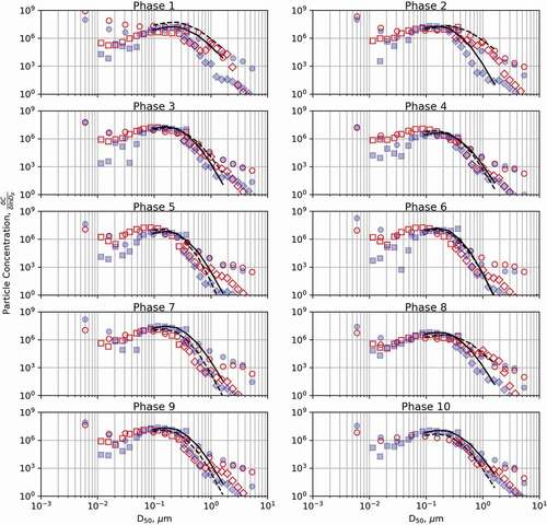
It is clear that there is some disagreement between the ELPI+ measurements and the SMPS and OPS measurements; all three instruments largely agree within the AMP regime, however the ELPI+ results diverge from the SMPS results in the UFP regime and diverge from the OPS results in the CMP regime. The size resolved particle number concentration measurements from the ELPI+ are typically higher than the SMPS and OPS measurements where they overlap. This result is not unexpected given the different measuring techniques employed within the instrumentation, and the different resolution of the instrumentation within the given particle size regimes. Further there is some uncertainty in the use of the ELPI+, namely, particle bounce and charge efficiency, which could cause diverging results (Pagels et al. 2005). Of these two issues, particle bounce is the most likely to cause increased particle counts, however due to the sticky nature of the aerosol, particles bouncing of the stages is unlikely.

Despite the aforementioned differences in magnitude the combined results point toward a trimodal PSD with one mode in each of the UFP, AMP, and CMP regimes. The mode in the UFP regime is supported by the steep shoulder seen in the ELPI+ results between 0.006 and 0.030 µm; this same evidence is mirrored in the SMPS results, which show a less drastic shoulder between 0.010 and 0.020 µm. In the case of HH B, the SMPS results also show a peaked distribution centered in the UFP regime. The AMP mode is clearly present in the results of all three instruments. In the case of the ELPI+ data, both sides of the distribution peak are clearly resolved. In the case of the SMPS data the left shoulder is defined, and in the case of the OPS, the right shoulder is defined. The mode in the CMP regime is supported by the broad shoulder extending out from the AMP distribution, evidenced in the ELPI+ and OPS results.

With regard to the accuracy of the fitting procedure, a least-squares-regression technique was used to calculate the standard deviation between the ELPI+ data and the modeled fit within the AMP mode window. The calculated standard deviation was approximately three times the N₁ parameter for all phases for both HHs.

The UFP, AMP, and CMP regime PSD parameters calculated from the ELPI+ data are shown in Table 4. The UFP, AMP, and CMP PSDs calculated from the ELPI+ data are similar across HHs when comparing overall test averages, however each HH shows comparatively large variations between different phases. A detailed analysis of the AMP regime PSD is discussed below; An in-depth analysis of the UFP and CMP regime PSD will be forgone due to inconsistencies between the measurements in the UFP and CMP range comparing the different instrumentation, concerns regarding the d_g in the UFP regime being smaller than the measurement window of the ELPI+ and SMPS and concerns due to the loading effects on the ELPI+ measurements in the CMP regime. The PSD parameters calculated from the SMPS and OPS data are given in the appendices and are not discussed below.

For HH A, d_g1 ranged between 0.130 and 0.212 µm with an overall appliance average value of 0.160 µm; σ_g1 spanned between 1.50 and 1.81 with an overall appliance average value of 1.71, which indicates a polydisperse aerosol within the AMP regime. For HH A larger average d_g1ʹs were found during Phases 1, 2 and 8. These phases also corresponded to the largest σ_g1ʹs, indicating the PSD was broader during these phases than during phases where smaller d_g1s were observed. The overall HH average d_g1 value seems to poorly represent the full dataset, and instead forms two distinct groupings. Kinsey et al. found similar results and postulated the correlation of high particle concentration with high d_g1 was due to the enhancement of coagulation processes by the presence of high concentrations of UFP aerosol. Another possible explanation is incomplete combustion. Incomplete combustion is typically expected during fuel loading events due to high moisture content of fuel, which occurs during Phases 1 and 2, and similarly during low output conditions such as Phase 8 due to low airflow conditions. Incomplete combustion typically produces high concentrations of volatile organic compounds, which could contribute to particle growth, thus explaining the larger d_g1 values. This explanation is corroborated by findings from Johansson et al., who found that PNC and total organic carbon are linearly correlated (Johansson et al. 2004). A notable exception occurs during the Phase 7. That phase includes a fuel addition and maintains a high heat output; however, a phase d_g1 below the appliance average d_g1 was observed. The AMP PSD results during this phase are very similar to the previous two phases. This suggests that ignition of the fresh fuel during Phase 7 was more gradual than during the Phases 1 and 2, which prevented a drastic change in AMP PSD. This finding indicates that firebox conditions and heat output can make a difference in the character of particulate emissions during fuel additions.

For HH B, the d_g1 ranged between 0.145 and 0.188 µm, with an overall HH average of 0.154 µm. The test average d_g1 value was more representative for HH B; only the pre-burn phase exhibited a d_g1 significantly larger than the appliance average, with a value of 0.188 µm. When compared by phase the d_g1ʹs for HH B were larger than for HH A in most cases. The σ_g1 values for HH B ranged between 1.56 and 1.73 with an average value of 1.59, a similar range to HH A. Larger than average d_g1ʹs were found in Phase 1 and 10, and the σ_g1 values were similarly larger during these periods.

Overall, the PSD results from both HHs are consistent with literature values found for other HH devices. For example, Kinsey et al. found a bimodal particle size distribution with modes in the UFP and AMP regimes for similar HH appliances burning the same type of fuel (red oak). In this article, Kinsey reported aerodynamic median particle diameters between 0.084 and 0.187 µm within the AMP regime (Kinsey et al. 2012).

Conclusion

Over the course of this investigation, the data showed that the PNC₁₀ mean value is significantly elevated during phases that include loading events; the PNC₁₀ concentrations are dependent on HH output, HH PNC₁₀ is dominated by UFPs while CMPs represent less than 1% of PNC₁₀, and within the accumulation mode, the d_g is dependent on loading events and on heat output. Each of these findings is discussed in further detail below. Figure 3 shows that there are differences between cold and hot starts, namely cold-start emissions, as in Phase 1, are higher than those during warm starts, occurring in Phase 2 and 7. It is also apparent that there is variability in PNC₁₀ between HHs even during repeated warm start fueling events. This is evidenced by the fact that HH A consistently produced decreased emissions with subsequent fueling, while HH B produced comparable PNC₁₀ emissions across each of these phases. From a regulatory test methodology perspective, this is important as many current test methods require testing of only hot starts and do not include multiple fuel loads.

The trends in PNC₁₀ between phases illustrate another point. Current HH certification testing mandates that a boiler be operated according to one heating category (<15, 16–25%, 26–50%, 100%) for, however, long it takes to burn one fuel charge. In contrast, an HH in the field must adapt to a changing heat demand, which depends on the users’ habits, climate, weather, and a host of other factors. Conducting certification testing in the current manner ignores the effect of transient periods in heat output, which are likely to occur in actual use and have been shown to occur for PNC₁₀ using the test method employed here. Further, the current method allows the low heat load test to be replaced by a second medium-low test, a provision that has become the norm. Phase 8 had larger than average particle size for HH A, which means more massive particles are created during this condition, which could affect particle mass concentrations and emission rates. For HH B, Phase 8 and Phase 4 PNC₁₀ were different and followed a unique trend, suggesting that testing at both conditions is necessary to really understand low heat output emissions from the device.

These criteria result in a certification method, which does not adequately represent the HHs performance in output conditions it will likely operate in, which are different than other heat output categories in terms of PNC₁₀.

Appliance PNC₁₀ measurements are dominated by particles less than 0.100 µm. AMPs between 0.100 and 1 µm account for less 30% of PNC₁₀, and CMPs between 1 and 10 µm account for less than 1% of the total PNC₁₀. Current certification testing is based on gravimetric measurement techniques. Filter efficiencies for UFP and small accumulation mode particles are low for certain filter types especially in the 0.100–0.200 µm range, which this analysis has found the geometric mean aerodynamic diameter of the AMP particle mode fall into. These finding suggests gravimetric sampling methods may inadequately measure these particles. These results also show that large AMPs are formed during cold-start fuel additions, which occur during Phase 1 and to a lesser extent Phase 2. This behavior is significantly different than during steady-state combustion. Further, the duration of this period and magnitude of emissions differ between HHs. In some cases, current certification tests do not include fuel additions, which suggests some HHs are being sold, which are not optimized for these conditions.

The results presented here describe the size-resolved concentration and average diameter of PM from two HH operated according to a load profile test method. Specifically, in this investigation, the mean PNC₁₀ concentrations were determined, and the PSD of the emitted particles were described using a tri-modal lognormal distribution in each phase. Our findings suggest that HH can significantly impact PNC₁₀ at the local scale and that the current certification test method for these units may be deficient in quantifying the magnitude of particulate emission from these devices, especially during and immediately after a cold-start.

Data availability

The data that support the findings of this study are available from the corresponding author, JL, upon reasonable request.

Acknowledgment

The authors would like to acknowledge everyone at the Energy Conversion Group at Brookhaven National Laboratory (BNL) for organizing the experiments and operating the appliances and Northeast States for Coordinated Air Use Management (NESCAUM) for developing the test method used in this study. Financial support from New York State Energy Research Development Authority (NYSERDA) has made this work possible. This research was funded through NYSERDA Agreement 63033.

Disclosure statement

No potential conflict of interest was reported by the author(s).

Supplementary material

Supplemental data for this paper can be accessed on the publisher’s website

Additional information

Funding

This work was supported by the New York State Energy Research and Development Authority [63033].

Notes on contributors

Jake Lindberg

Jake Lindberg is a recent doctoral graduate at Stony Brook University in the Chemical and Molecular Engineering Department in Stony Brook, New York, USA and works closely with the Energy Conversion Group, at Brookhaven National Laboratory in Upton, New York, USA.

Nicole Vitillo

Nicole Vitillo is a research scientist at the New York State Department of Health, in the Center for Environmental Health, Bureau of Toxic Substance Assessment, Exposure Characterization and Response Section, in Albany, New York, USA.

Marilyn Wurth

Marilyn Wurth is a research scientist at the New York State Department of Environmental Conservation, in the Emissions Measurement Research Group within the Division of Air Resources, Bureau of Mobile Sources & Technology Development in Albany, New York, USA.

Brian P. Frank

Brian P. Frank is the section chief of the Emissions Measurement Research Group at the New York State Department of Environmental Conservation, Division of Air Resources, Bureau of Mobile Sources & Technology Development in Albany, New York, USA.

Shida Tang

Shida Tang is a research scientist at the New York State Department of Environmental Conservation, in the Emissions Measurement Research Group within the Division of Air Resources, Bureau of Mobile Sources & Technology Development in Albany, New York, USA.

Gil LaDuke

Gil LaDuke is a research scientist at the New York State Department of Environmental Conservation, in the Emissions Measurement Research Group within the Division of Air Resources, Bureau of Mobile Sources & Technology Development in Albany, New York, USA.

Patricia Mason Fritz

Patricia Mason Fritz is the section chief of the Exposure Characterization and Response Section at the New York State Department of Health, in the Center for Environmental Health, Bureau of Toxic Substance Assessment, in Albany, New York, USA.

Rebecca Trojanowski

Rebecca Trojanowski is a research scientist at Brookhaven National Laboratory, in the Interdisciplinary Science Department, Energy Conversion Group, in Upton, New York, USA, and is a doctoral candidate at Columbia University in the Department of Earth and Environmental Engineering, in New York, New York, USA.

References

- Ahmadi, M., J. Minot, G. Allen, and L. Rector. 2020. Investigation of real-life operating patterns of wood-burning appliances using stack temperature data. Journal of the Air & Waste Management Association 70 (4):393–409. doi:10.1080/10962247.2020.1726838.
- Allen, G., P. J. Miller, L. J. Rector, M. Brauer, and J. U. Su. 2011. Characterization of valley winter woodsmoke concentrations in northern NY using highly time-resolved measurements. Aerosol and Air Quality Research 11 (5):519–30. doi:10.4209/aaqr.2011.03.0031.
- Allen, G., and L. Rector. 2020. Characterization of Residential Woodsmoke PM2.5 in the Adirondacks of New York. Aerosol and Air Quality Research. 2419–32.
- Berry, C. “Increase in wood as main source of household heating most notable in the Northeast.” EIA. 17 March 2014. https://www.eia.gov/todayinenergy/detail.php?id=15431.
- Gibbs, R., and T. Butcher. 2010. Staged combustion biomass boilers: Linking high-efficiency combustion technology to regulatory test methods. Albany: New York State Energy Research and Development Authority (NYSERDA).
- Gonçalves, C., C. Alves, A. P. Fernandes, C. Monteiro, L. Tarelho, M. Evtyugina, C. Pio. 2011. Organic compounds in PM2.5 emitted from fireplace and wood stove combustion of typical Portuguese wood species. Atmospheric Environment. 45 (27):4533–45. doi:10.1016/j.atmosenv.2011.05.071.
- Hays, M. D., N. D. Smith, J. Kinsey, Y. Dong, and P. Kariher. 2003. Polycyclic aromatic hydrocarbon size distributions in aerosols from appliances of residential wood combustion as determined by direct thermal desorption—GC/MS. Journal of Aerosol Science 34 (8):1061–84. doi:10.1016/S0021-8502(03)00080-6.
- Hinds, W. C. 1982. Particle size statistics. In Aerosol technology: Properties, behavior, and measurement of airborne particles, ed. W. C. Hinds, 69–103. New York: John Wiley & Sons.
- Johansson, L. S., B. Leckner, L. Gustavsson, D. Cooper, C. Tullin, and A. Potter. 2004. Emission characteristics of modern and old-type residential boilers fired with wood logs and pellets. Atmospheric Environment 38 (25):4183–95. doi:10.1016/j.atmosenv.2004.04.020.
- Kinsey, J. S., A. Touati, T. L. B. Yelverton, J. Aurell, S.-H. Cho, W. P. Linak, B. K. Gullett. 2012. Emissions characterization of residential wood-fired hydronic heater technologies. Atmospheric Environment 63:239–49. doi:10.1016/j.atmosenv.2012.08.064.
- Kleeman, M. J., J. J. Schauer, and G. R. Cass. 1999. Size and composition distribution of fine particulate matter emitted from wood burning, meat charbroiling, and cigarettes. Environmental Science & Technology. 33:3516–23.
- Kocbach Bølling, A., Pagels, J., Yttri, K. E., Barregard, L., Sallsten, G., Schwarze, P. E., Boman, C. 2009. Health effects of residential wood smoke particles: the importance of combustion conditions and physiochemical particle properties. Particle and Fiber Toxicology 6 (6):29. doi:10.1186/1743-8977-6-29. PMID: 19891791; PMCID: PMC2777846.
- Kotchenruther, R. A. 2016. Source apportionment of PM2.5 at multiple Northwest U.S. sites: Assessing regional winter wood smoke impacts from residential wood combustion. Atmospheric Environment. 142:210–19. doi:10.1016/j.atmosenv.2016.07.048.
- Lillieblad, L., Szpila, A., Strand, M., Pagels, J., Rupar-Gadd, K., Gudmundsson, A., and Sanati, M. 2004. Boiler operation influence on the emissions of submicrometer-sized particles and polycyclic aromatic hydrocarbons from biomass-fired grate boilers. Energy & Fuels. 18:410–17.
- Lindberg, J., Wurth, M., Frank, B., Tang, S., LaDuke, G., Trojanowski, R., Butcher, T., Mahajan, D. 2022. Realistic operation of two residential cordwood fired appliances - Part 3: Black and brown carbon emissions. Review.
- Naeher, L. P., M. Brauer, M. Lipsett, J. T. Zelikoff, C. D. Simpson, J. Q. Koenig, K. R. Smith. 2007. Woodsmoke health effects: A review. Inhalation Toxicology. 19 (1):67–106. doi:10.1080/08958370600985875.
- Noonan, C. W., T. J. Ward, and E. O. Semmens. 2015. Estimating the number of vulnerable people in the United States exposed to residential wood smoke. Environmental Health Perspectives 123 (2):A30. doi:10.1289/ehp.1409136. PMID: 25642637; PMCID: PMC4314255.
- NYSERDA. 2008. “Assessment of Carbonaceous PM2.5 for New York and the region.”
- NYSERDA. 2012. “Environmental, Energy Market, and Health Characterization of Wood-Fired Hydronic Heater Technologies.”
- NYSERDA. 2016. “New York State: Wood heat report: An energy, environmental, and market assessment.”
- Obernberger, I., T. Brunner, and G. Barnthaler. 2007. “Fine particulate emissions from modern Austrian small-scale biomass combustion plants.” 15th European Biomass Conference & Exhibition Berlin, 1546–57.
- Pagels, J., A. Gudmundsson, E. Gustavsson, L. Asking, and M. Bohgard. 2005. Evaluation of aerodynamic particle sizer and electrical low-pressure impactor for unimodal and bimodal mass-weighted size distributions. Aerosol Science and Technology 39 (9):871–87. doi:10.1080/02786820500295677.
- Penn, S. L., S. Arunachalam, M. Woody, W. Heiger-Bernays, Y. Tripodis, and J. I. Levy. 2017. Estimating state-specific contributions to PM 2.5 - and O 3 -related health burden from residential combustion and electricity generating unit emissions in the United States. Environmental Health Perspectives 125 (3):324–32. doi:10.1289/EHP550.
- Pettersson, E., C. Boman, R. Westerholm, D. Bostrom, and A. Nordin. 2011. Stove performance and emission characteristics in residential wood log and pellet combustion, part 2: Wood stove. Energy and Fuels 25 (1):315–25. doi:10.1021/ef1007787.
- Rector, L., G. Allen, and P. Johnson. 2006. Assessment of outdoor wood-fired boilers. Boston, MA: Northeast States for Coordinated Air Use Management (NESCAUM).
- Rector, L., P. J. Miller, S. Snook, and M. Ahmadi. 2017. Comparative emissions characterization of a small-scale wood chip-fired boiler and an oil-fired boiler in a school setting. Biomass and Bioenergy 107:254–60. doi:10.1016/j.biombioe.2017.10.017.
- Schmidl, C., M. Luisser, E. Padouvas, L. Lasselsberger, M. Rzaca, C. Ramirez-Santa Cruz, M. Handler, G. Peng, H. Bauer, H. Puxbaum, et al. 2011. Particulate and gaseous emissions from manually and automatically fired small scale combustion systems. Atmospheric Environment. 45(39):7443–54. doi:10.1016/j.atmosenv.2011.05.006.
- Schrieber, J., R. Chinery, J. Snyder, E. Kelly, E. Valerio, and E. Acosta. 2005. Smoke gets in your lungs: outdoor wood boilers in New York State. https://shwec.engr.wisc.edu/wp-content/uploads/sites/711/2015/08/NYRptRev08.pdf
- Sehlstedt, M., R. Dove, C. Boman, J. Pagels, E. Swietlicki, J. Löndahl, R. Westerholm, J. Bosson, S. Barath, A. F. Behndig, et al. 2010. Antioxidant airway responses following experimental exposure to wood smoke. Particle and Fiber Toxicology 7 (1). doi: 10.1186/1743-8977-7-21.
- Shen, G., M. Xue, S. Wei, Y. Chen, B. Wang, R. Wang, H. Shen, W. Li, Y. Zhang, Y. Huang, et al. 2013. Influence of fuel mass load, oxygen supply and burning rate on emission factor and size distribution of carbonaceous particulate matter from indoor corn straw burning. Journal of Environmental Sciences. 25 (3):511–19. doi:10.1016/S1001-0742(12)60191-0.
- Sigsgaard, T., B. Forsberg, I. Annesi-Maesano, A. Blomberg, A. Bølling, C. Boman, J. Bønløkke, M. Brauer, N. Bruce, M.-E. Héroux, et al. 2015. Health impacts of anthropogenic biomass burning in the developed world. European Respiratory Society. 46(6):1577–88. doi:10.1183/13993003.01865-2014.
- Squizzato, S., Masiol, M., Emami, F., Chalupa, D. C., Utell, M. J., Rich, D. Q., & Hopke, P. K. 2019. Long-term changes of source apportioned particle number concentrations in a metropolitan area of the Northeastern United States. Atmosphere 10:27. doi:10.3390/atmos10010027.
- Trojanowski, R., and V. Fthenakis. 2019. Nanoparticle emissions from residential wood combustion: A critical literature review, characterization, and recommendations. Renewable and Sustainable Energy Reviews 103:515–28. doi:10.1016/j.rser.2019.01.007.
- Trojanowski, R., Lindberg, J., Butcher, T., Fthenakis, V. 2022. Realistic operation of two residential cordwood fired appliances - Part 1: Particulate mass and gaseous emissions.
- United States Census Bureau. “American Housing Survey (AHS).” 2 July 2021. https://www.census.gov/programs-surveys/ahs.html.
- U.S. EPA. 2017. “Test method 28 OWHH for measurement of particulate emissions and heating”.
- U.S. EPA. 1998. “Residential wood combustion technology review volume 1. Technical Report.”
- U.S. EPA. 2019. “Integrated Science Assessment (ISA) for particulate matter (final report, 2019).”
- Vicente, E. D., M. A. Duarte, A. I. Calvo, T. F. Nunes, L. A. C. Tarelho, D. Custódio, C. Colombi, V. Gianelle, A. Sanchez de la Campa, C. A. Alves. 2015a. Influence of operating conditions on chemical composition of particulate matter emissions from residential combustion. Atmospheric Research 166:92–100. doi:10.1016/j.atmosres.2015.06.016.
- Vicente, E. D., M. A. Duarte, A. I. Calvo, T. F. Nunes, L. Tarelho, and C. A. Alves. 2015b. Emission of carbon monoxide, total hydrocarbons and particulate matter during wood combustion in a stove operating under distinct conditions. Fuel Processing Technology 131:182–92. doi:10.1016/j.fuproc.2014.11.021.
- Wang, Y., P. K. Hopke, X. Xia, O. Rattigan, D. C. Chalupa, and M. J. Utell. 2012. Source apportionment of airborne particulate matter using inorganic and organic species as tracers. Atmospheric Environment 55:525–32. doi:10.1016/j.atmosenv.2012.03.073.
- Ward, T., B. Trost, J. Conner, J. Flanagan, and R. K. M. Jayanty. 2012. source apportionment of PM2.5 in a subarctic airshed - fairbanks, Alaska. Aerosol and Air Quality Research 12 (4):536–43. doi:10.4209/aaqr.2011.11.0208.
- Weichenthal, S., R. Kulka, E. Lavigne, D. van Rijswijk, M. Brauer, P. J. Villeneuve, D. Stieb, L. Joseph, R. T. Burnett. 2017. Biomass burning as a source of ambient fine particulate air pollution and acute myocardial infarction. Epidemiology. 28 (3):329–37. doi:10.1097/EDE.0000000000000636.
- Win, K. M., and T. Persson. 2014. Emissions from residential wood pellet boilers and stove characterized into start-up, steady operation, and stop emissions. Energy & Fuels 28(4):2496–505.