Future year (2028) source apportionment modeling to support Regional Haze Rule planning in the western U.S.

ABSTRACT

The Western Regional Air Partnership (WRAP) has developed a modeling platform to simulate the formation of haze-causing particles that impact federally-protected lands in the western United States. To assist state air quality planners in determining which emission sources are likely candidates for future mitigation, several source apportionment scenarios were evaluated, and two sets of results for the year 2028 are presented here: 1) a “high-level important regional sources” version, with broad emission categories (i.e. U.S. anthropogenic, international anthropogenic, natural, and fires), and 2) a “low-level anthropogenic emission sources within individual states” version, which refines the U.S. anthropogenic contribution to specific emission sectors within individual WRAP region states. Eight examples are discussed, which reflect the variation in source apportionment results at national parks, wilderness areas, and wildlife refuges in the western U.S. and suggest which emission sectors are candidates for mitigation to improve future visibility. In 2028, the contribution of domestic anthropogenic emissions at the eight sites ranges from 17% to 58%, with significant impacts from oil and gas production, fossil fuel electric generation, and federally-regulated mobile sources. The contribution from international anthropogenic sources can also be considerable, and ranges from 17% to 43%. Most sectors that are emitting sulfur dioxide (SO₂) and nitrogen oxides (NO_x), which are the two most likely particle precursors to be curtailed in the states’ Regional Haze plans, are declining. For example, in the 13 contiguous WRAP region states, NO_x emissions from on-road mobile sources and electric generating units (EGUs) declined by 738 kton/yr (29% decrease) and 65 kton/yr (31% decrease), respectively, in 2028 as compared to current emission estimates, and SO₂ emissions from EGUs declined by 42 kton/yr (29% decrease). NO_x emissions from oil and gas development also declined by 25 kton/yr (9% decrease) but rose for SO₂ emissions by 12 kton/yr (20% increase).

Implications: The goal of the Regional Haze Rule (RHR) is to improve visibility at federally-protected areas, and to eventually arrive at natural conditions by the year 2064. Source apportionment tools within regional air quality models are useful for identifying which emission regions and sectors are contributing to haze-causing particles and can indicate to air quality planners where additional emission controls may be warranted.

Introduction

The Regional Haze Rule (RHR) is now over twenty years old, and states are in the second round of developing State Implementation Plans (SIPs) for submission to the U.S. Environmental Protection Agency (U.S. EPA) to promote better visibility in federal Class I areas (CIAs) (U.S. EPA 1999). Class I federal lands include national parks, monuments, and wilderness areas that are granted special air quality protections under Section 162(a) of the Clean Air Act. The RHR instructs states to submit plans every 10 years that demonstrate reasonable progress toward the goal of achieving natural visibility conditions on the most impaired days by the year 2064. In 2017, EPA revised the metric to track progress in achieving better visibility, with an emphasis on the role of manmade emissions as stated in the 1977 Clean Air Act Amendments (U.S. EPA 2017; Gantt et al. 2018). Instead of considering the 20% observed haziest days in each year (as was done in the first round of RHR SIPs), states are now to track visibility progress on the 20% of days with the highest anthropogenic impairment estimates (i.e., “most impaired days”, or MID). This is especially important at CIAs in the western U.S., where episodes of elevated carbonaceous particles or crustal material, attributed to wildfires or dust storms, respectively (Hand et al. 2013; 2016), often dominate particle loads on the haziest days. The use of the haziest days metric made it more difficult for states to demonstrate progress in reducing anthropogenic impairment from reductions in U.S. anthropogenic emissions, as intended by the RHR, as visibility in CIAs is frequently and significantly impaired by dust and smoke.

Visibility conditions at CIAs are tracked using particle measurements from the Interagency Monitoring of Protected Visual Environments (IMPROVE; Solomon et al. 2014) network. IMPROVE measures concentrations of fine particles (PM2.5, i.e., particulate matter less than 2.5 µm in size) of ammonium sulfate (AmmSO4), ammonium nitrate (AmmNO3), organic matter carbon (OMC), elemental carbon (EC), crustal material (fine soil), and sea salt. Coarse particles (CM, i.e., particulate matter between 2.5 µm and 10 µm in size) are also measured. The visibility metric used in this study is particulate light extinction, expressed as inverse megameters (Mm⁻¹), and is calculated with the revised IMPROVE equation (Pitchford et al. 2007). This equation relates the concentration of the seven particle species listed above to an estimated particle light extinction. The IMPROVE program collects a 24-hour sample every third day, from which the 20% MID over a calendar year are identified (U.S. EPA 2019). This collection of MID dates, defined by the observational record, is often unique for each CIA and forms the foundation of further analyses to assess how visibility is evolving on the 20% MID at an individual site.

To support planners in the western U.S. with their second round of RHR SIP development, the Western Regional Air Partnership (WRAP) developed a modeling platform using the Comprehensive Air Quality Model with Extensions (CAMx; Ramboll 2020a) to estimate which emission sources contribute to haze. This approach is known as a source apportionment and can be used to examine the role of anthropogenic vs. natural emission sources, contributions of individual states, or specific sectors within the emission inventory. In practice, this new emphasis on the MID metric (as opposed to the haziest days) has resulted in a focus on AmmSO4 and AmmNO3 particles, given that their precursors (sulfur dioxide (SO₂) and nitrogen oxides (NO_x), respectively) are largely associated with anthropogenic sources and are considered the most amenable to potential emission reductions, and is consistent with the updated EPA guidance on tracking the most anthropogenically-impaired days. CAMx has been used extensively in source apportionment studies of AmmSO4 and AmmNO3 (Aksoyoglu et al. 2017; Brewer et al. 2019; Koo et al. 2009; Pepe et al. 2019; U.S. EPA 2019).

A key provision of the RHR is assessing the degree of projected future visibility improvement (termed Reasonable Progress Goal, or RPG) at each CIA. For the second round of RHR SIP development, this future year is defined as 2028. To assist planners in their efforts of identifying the most effective emission mitigation strategies to achieve these 2028 RPGs, the WRAP modeling platform estimated a source apportionment for this future year, with updates to the emission inventory that reflect anticipated reductions. Several broad emission categories were defined (e.g., anthropogenic emissions from U.S. sources, natural emissions, wildfires), and then further refined to consider the SO₂ and NO_x emissions from individual WRAP region states with respect to specific sectors (e.g., electric power generation, oil and gas extraction, mobile sources). The other IMPROVE species (OMC, EC, fine soil, CM, sea salt) are also considered in the source apportionment but do not receive the more detailed sector-specific treatment as AmmSO4 and AmmNO3. This is not to discount the role of the other IMPROVE species, but rather to acknowledge that, for example, mitigating high levels of organic particles associated with wildfires, or soil particles from dust storms, may not be a feasible prospect for state air quality planners.

This paper provides an overview of the CAMx modeling system and its application to developing source apportionment results for 2028 in support of RHR SIP development for WRAP region states. Although not presented here, several other analyses were conducted by the WRAP to assist air quality planners with their SIPs, including:

• Weighted Emissions Potential/Area of Influence (WEP/AOI) Analyses: By using back trajectories to estimate the area of influence of emission sources, and then overlaying these results with SO₂ and NO_x emissions, source regions and individual point sources can be ranked by their probability of contributing to visibility impairment at downwind CIAs (WRAP 2020a).

• Dynamic Model Evaluation: To evaluate CAMx’s ability to replicate observed particle concentrations in response to changes in emission inventories, a dynamic model evaluation was conducted. In addition to the current and 2028 emission inventories that were developed by WRAP, an additional inventory for 2002 was ‘hindcast’ from the current inventory and then used by CAMx to estimate particle concentrations during 2000-2004 (Morris et al. 2022; WRAP 2020b).

• Future Fire Scenarios: Wildfire activity in the western U.S. is expected to increase in both intensity and duration for a variety of reasons, including accumulated fuels, climate change, drought, and other factors. To help planners anticipate this future fire regime, CAMx runs were conducted using specialized scenarios to evaluate impacts from future wild and prescribed fires (Air Sciences 2020; WRAP 2021a).

WRAP developed a Technical Support System (TSS; https://views.cira.colostate.edu/tssv2/) that includes monitoring, emissions, modeling, and analysis products that state planners can use as the technical basis for their RHR SIPs. The source apportionment results presented in this paper are from the WRAP TSS, and many more tools are available here for evaluating haze trends, additional source apportionment simulations, and estimated current and future emission inventories.

Methods

CAMx configuration

CAMx version 7 (Ramboll 2020a) was used for this study. Configuration options, model inputs, and a performance evaluation can be found at WRAP (2020c); details that are most relevant to the 2028 source apportionment results are presented here.

For this study, a year-long CAMx simulation was desired, and a key consideration in the initial development of the modeling platform was specifying which calendar year to use for the “base case” simulation. Three recent candidate years (2014–2016) were considered for their suitability in creating a modeling platform that is broadly representative of typical meteorological and air pollution conditions, and applicable to a wide range of potential air quality issues of interest to the WRAP. 2014 was chosen as the most representative year (Ramboll 2018), and was the starting point for developing the base case CAMx simulation.

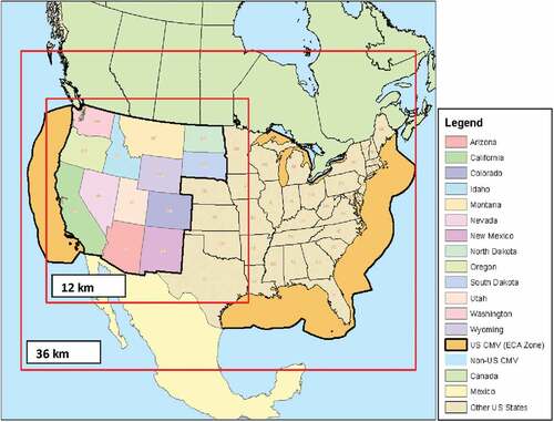
CAMx model domains are shown in Figure 1 and consist of an outer 36 km domain that covers the conterminous U.S., along with southern Canada and northern Mexico, and an inner 12 km domain for the western U.S. that is nested within the outer 36 km domain. Dynamic two-way nesting was used, so recirculation of pollutants between the inner and outer domains was captured. Meteorological inputs were simulated with the Weather Research Forecast model (WRF; Skamarock et al. 2008), and performance was evaluated against 2014 meteorological measurements (Bowden, Talgo, and Adelman 2016). Boundary conditions, which were specified at the periphery of the 36 km domain, were provided by the GEOS-Chem global chemical transport model (Bey et al. 2001; WRAP 2019).

Figure 1. Camx nested 12 km and 36 km model domains, and the 13 WRAP states that were evaluated in the low-level source apportionment. Other source regions include the non-WRAP states, Canada, Mexico, and U.S. And non-U.S. commercial marine vehicles.

A considerable amount of effort in this study was devoted to improving and projecting emission inventories, especially for sources within the WRAP region states. Emissions for the 2014 base case, a representative baseline period of 2014–2018, and projections to 2028 were developed (WRAP 2021b). The inventory consists of many different source sectors, such as fossil fuel electric generating units (EGUs), industrial point sources, on-road mobile emissions, and oil and gas development. Emissions from biogenic and natural sources, as well as fires, are also included. The starting point for many of these sectors was the 2014v2 National Emission Inventory (U.S. EPA 2018) or the 2016v1 North American Emissions Modeling Platform (U.S. EPA 2021). Some emission sectors within the WRAP region, such as oil and gas development and fires, were further refined to improve accuracy (WRAP 2021b). Emissions defined as natural within the modeling domain, and those from outside the WRAP region, were generally held constant at current levels.

An extensive model performance evaluation for the 2014 base case is discussed in WRAP (2020c), and considers the IMPROVE particle species described above, as well as ozone. With regard to particulate sulfate (SO4) and nitrate (NO3), which are a primary focus of the anthropogenic source apportionment simulations, the model’s skill generally falls within the prescribed performance metrics, as presented in WRAP (2020c).

Overview of CAMx simulations

Arriving at the final version of the 2014 base case CAMx simulation was an iterative process, and required several refinements, including updates to the emission inventory, improved boundary conditions, incorporating bi-directional ammonia fluxes, and several sensitivity simulations (WRAP 2020c). Once adequate model performance was achieved, additional CAMx runs were developed to estimate how current and future year U.S. anthropogenic emissions affect visibility in the western U.S. These CAMx runs include:

1. ‘Representative baseline’ simulation (RepBase2), where U.S. anthropogenic emissions representative of the 2014-2018 period are evaluated,

2. 2028 ‘on the books’ simulation (2028OTBa2), where U.S. anthropogenic emissions are forecast to reflect legislated, administrative rulemaking mandates, and permit-mandated reductions, principally to SO₂ and NO_x emissions, and

3. 2028 ‘potential additional controls’ simulation (2028PAC2), where additional emission controls, beyond those specified in 2028OTBa2, are considered for SO₂ and NO_x emissions from the WRAP region states.

To maintain consistency in evaluating the role of U.S. anthropogenic emissions on regional haze, the same 2014 meteorology, boundary conditions, and biogenic emissions were used for all CAMx model runs. Fire emissions were held constant to the levels specified in the representative baseline inventory. The results presented here are from the 2028 “on the books” simulation (2028OTBa2, and hereafter referred to as simply “2028” or “future year”); the interested reader can find details about the other CAMx runs at WRAP (2021c).

2028 SO₂ and NO_x emission inventories in the 13 contiguous WRAP region states

As mentioned earlier, one of the goals of this paper is to examine the role of anthropogenic SO₂ and NO_x emissions from the WRAP region states on future haze impacts with regard to AmmSO4 and AmmNO3, and to identify which source sectors are having the largest effect at CIAs in the western U.S. Figures 2 and 3 show SO₂ and NO_x emissions, respectively, for the 13 contiguous WRAP region states. Nine anthropogenic source sectors are presented: 1) EGUs, 2) other industrial point sources (non-EGUs), 3) oil and gas point sources, 4) oil and gas area sources, 5) on-road mobile emissions, 6) non-road mobile emissions, 7) rail emissions, 8) commercial marine emissions, and 9) remaining anthropogenic emissions. These nine sectors account for 249 kton of SO₂ and 1,327 kton of NO_x emitted by the 13 WRAP region states in 2028. For clarity, some of the source categories that make small contributions to anthropogenic SO₂ and NO_x emissions (e.g., fugitive dust, residential wood combustion), or are not controllable (e.g., lightning NO_x, wildfires) are omitted in Figures 2 and 3.

Figure 2. (a) Total 2028 anthropogenic SO2 emissions from the 13 contiguous WRAP region states, and (b) individual WRAP region state contributions.

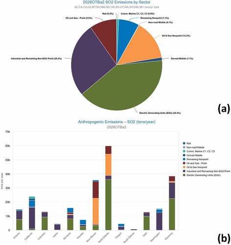
Figure 3. (a) Total 2028 anthropogenic NOx emissions from the 13 contiguous WRAP region states, and (b) individual WRAP region state contributions.

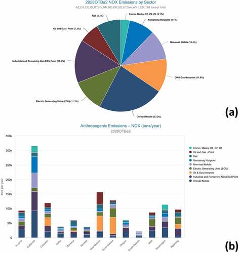
Of the nine anthropogenic sectors, EGUs are the largest source of SO₂ emissions at 101 kton/yr (40.1%), followed by other industrial point sources at 66 kton/yr (26.4%) and oil and gas production (point + area) at 59 kton/yr (23.8%) (Figure 2(a)). North Dakota and Wyoming account for the largest SO₂ emissions from EGUs, followed by Utah, Colorado, Montana, and Arizona. North Dakota and New Mexico have significant SO₂ emissions from oil and gas sources. NO_x emission sources are more uniformly distributed (Figure 3(a)), with on-road mobile sources estimated to be the single largest sector at 308 kton/yr (23.2%), closely followed by oil and gas production (point + area) at 253 kton/yr (19.0%). California is the single largest source to the on-road mobile sector, and also makes significant contributions to both the non-road mobile and commercial marine portions of the NO_x budget (Figure 3(b)). Over half of New Mexico’s anthropogenic NO_x emissions are attributed to oil and gas activity, which is also prominent in North Dakota, Colorado, Wyoming, and Utah. Non-industrial point sources and EGUs are the third and fourth leading categories, at 202 kton/yr (15.2%) and 151 kton/yr (11.3%), respectively.

High-Level and low-level source apportionment

Two approaches were taken for developing source apportionment estimates for the 112 WRAP region CIAs in the 13 contiguous WRAP states: 1) a “high-level” simulation, in which broad emission categories were considered, and their impacts on the seven IMPROVE species calculated, and 2) a “low-level” simulation, which further refined the anthropogenic SO₂ and NO_x emissions within the WRAP region states, yielding a more detailed evaluation of the role of these state-specific emissions on AmmSO4 and AmmNO3 (WRAP 2020d). The high-level source apportionment gives the general context as to which of the seven IMPROVE species are playing a dominant role with regard to visibility impairment, and whether they originate, for example, from anthropogenic versus natural emissions, or domestic versus international sources. The low-level source apportionment indicates to planners which anthropogenic source categories of SO₂ and NO_x emissions from each of the 13 contiguous WRAP region states could be promising candidates for mitigation, although controls at individual permitted point sources are subject to extensive additional analyses under the Regional Haze Rule.

Given the substantial overhead of simulating the reactive tracers within CAMx, the source apportionment runs are computationally expensive. This is especially true for the low-level source apportionment simulation, since there are significantly more regions and emission sectors that are tracked as compared to the high-level source apportionment. For this reason, only the future year inventory (2028) was modeled for the low-level source apportionment; these results will be described below, along with the 2028 high-level source apportionment. Although not discussed here, a high-level source apportionment was also conducted for the representative baseline inventory (RepBase2), which the interested reader can examine at the WRAP TSS.

For the high-level source apportionment, six emission categories are considered for each WRAP region CIA: 1) U.S. anthropogenic, 2) international anthropogenic, 3) natural, 4) U.S. wildfires, 5) U.S. prescribed wildland fires, and 6) fires from Canada and Mexico. For the low-level source apportionment, five source sectors that govern SO₂ and NO_x emissions, from each of the 13 WRAP region states, are analyzed: 1) fossil fuel EGUs, 2) non-EGU industrial sources, 3) oil and gas operations, 4) mobile sources, and 5) remaining anthropogenic sources. In an effort to accelerate and simplify the low-level source apportionment, some of emission sectors presented in Figures 2 and 3 are consolidated. For example, point and area emissions for oil and gas activities are combined, and mobile emissions are the collection of on-road, non-road, U.S. commercial marine, and aircraft emissions. The estimated individual contributions from the CAMx source apportionment simulation are converted from particle concentration (µg m⁻³) to particle light extinction (Mm⁻¹) using the revised IMPROVE equation (Pitchford et al. 2007).

Results and discussion

Overview

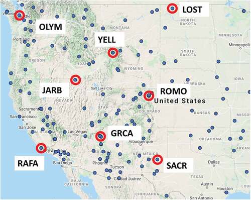
There are 112 CIAs in the 13 contiguous WRAP region states, which constitutes 75% of the national total, and these national parks, wilderness areas, and wildlife refuges vary widely in proximity to emission sources, topography, climate, and elevation. In practical terms, this means that drawing general conclusions about which emissions sources are most culpable in degrading future visibility is difficult. Instead, eight individual sites are presented (Figure 4), with the intent to illustrate the variety of source apportionment results within the WRAP region CIAs. Both the high-level and low-level source apportionment results for 2028 are considered. The four-letter naming convention used by IMPROVE is adopted here to abbreviate the names of the eight example CIAs, and additional information regarding the monitoring sites can be found at the WRAP TSS.

Figure 4. Class 1 areas within the CAMx 12 km model domain, and the eight example sites of Olympic National Park (‘OLYM’), Yellowstone National Park (‘YELL’), Lostwood National Wildlife Refuge (‘LOST’), Rocky Mountain National Park (‘ROMO’), Salt Creek Wilderness Area (‘SACR’), Jarbidge Wilderness Area (‘JARB’), Grand Canyon National Park (‘GRCA’), and San Rafael Wilderness Area (‘RAFA’).

Olympic National Park (‘OLYM’), Washington

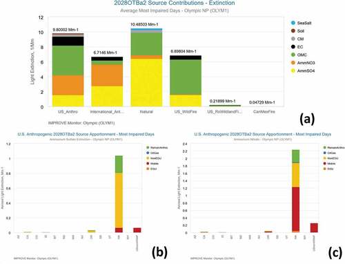
OLYM (Figure 5) is located on the Olympic Peninsula of western Washington and is near the Canadian border and the densely populated Puget Sound area, and approximately 90 km northwest of Seattle. Future year particle visibility impacts of 34.6 Mm⁻¹ are attributed to a combination of U.S. anthropogenic, international, natural, and wildfire emissions (Figure 5(a)). The sulfate and nitrate impacts from U.S. anthropogenic sources are primarily from emissions within Washington (Figures 5(b,c)), followed by a small contribution from Oregon sources. Washington’s mobile and non-EGU industrial sources are projected to contribute 1.2 Mm⁻¹ and 1.4 Mm⁻¹, respectively, to visibility impairment at OLYM. Fire impacts from U.S. wildfires are significant at 6.9 Mm⁻¹. Given OLYM’s proximity to the Pacific Ocean, the high AmmSO4 (6.4 Mm⁻¹) from natural sources is likely linked to biogenic dimethyl sulfide (DMS) emissions from ocean surface waters, and is potentially overestimated, as discussed in WRAP (2019).

Figure 5. Olympic National Park (‘OLYM’; Washington) high-level source apportionment results (a) and low-level source apportionment results for (b) AmmSO4 and (c) AmmNO3 from anthropogenic sources.

Yellowstone National Park (‘YELL’), Wyoming

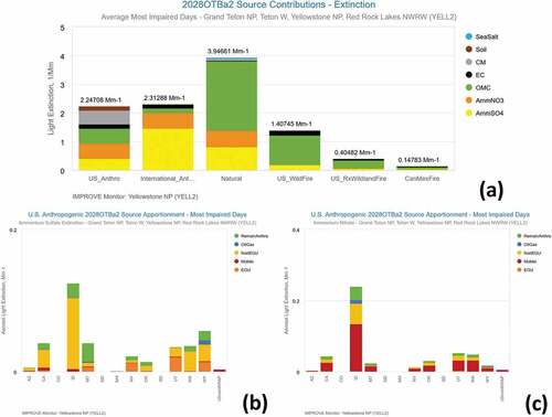
In contrast to OLYM, YELL (Figure 6), located in northwestern Wyoming, has significantly lower particle haze levels (10.5 Mm⁻¹) estimated in 2028, and is more isolated from urban emissions. Organic matter carbon from natural sources and fires plays a major role at this site (Figure 6(a)). The single largest contributor to AmmSO4 is international sources, which will be a reoccurring theme in several of these examples. AmmSO4 and AmmNO3 contributions from U.S. anthropogenic sources (Figures 6(b,c)) are distributed among numerous states, including Wyoming, Idaho, Utah, and California, and indicate the role of mobile sources for AmmNO3 impacts and a mix of EGUs and non-EGU industrial sources for AmmSO4.

Figure 6. Yellowstone National Park (‘YELL’; Wyoming) high-level source apportionment results (a) and low-level source apportionment results for (b) AmmSO4 and (c) AmmNO3 from anthropogenic sources.

Lostwood National Wildlife Refuge (‘LOST’), North Dakota

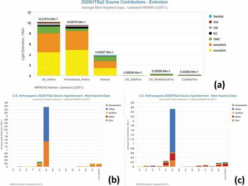
Located near the Canadian border in northern North Dakota, LOST (Figure 7) is another example of a CIA that is far removed from major urban areas. However, the role of U.S. anthropogenic and international emissions is more prominent here, and impacts from natural sources and fires are diminished, as compared to YELL (Figure 6(a)). The estimated future particle visibility impairment at LOST is 24.5 Mm⁻¹. AmmSO4 and AmmNO3 constitute the majority of the U.S. anthropogenic contribution, which is dominated by oil and gas development and electric power generation within North Dakota (Figures 7(b,c)), and to a lesser extent Montana and Wyoming. The combined AmmSO4 and AmmNO3 impact from oil and gas emissions is 3.9 Mm⁻¹. International contributions can likely be attributed to Canada given LOST’s location.

Figure 7. Lostwood National Wildlife Refuge (‘LOST’; North Dakota) high-level source apportionment results (a) and low-level source apportionment results for (b) AmmSO4 and (c) AmmNO3 from anthropogenic sources.

Rocky Mountain National Park (‘ROMO’), Colorado

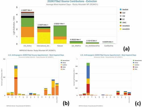
ROMO (Figure 8) is located in north-central Colorado, near the densely populated Front Range urban corridor, and approximately 90 km northwest of Denver. The bulk of the future particle impairment is due to U.S. anthropogenic sources (4.3 Mm⁻¹), followed by international (2.4 Mm⁻¹) and natural (2.5 Mm⁻¹) sources (Figure 8(a)). Fire impacts at ROMO are small. Most of the AmmSO4 and AmmNO3 is attributed to a variety of sources within Colorado (0.3 Mm⁻¹ and 0.9 Mm⁻¹, respectively), followed by contributions from Wyoming and Utah.

Figure 8. Rocky Mountain National Park (‘ROMO’; Colorado) high-level source apportionment results (a) and low-level source apportionment results for (b) AmmSO4 and (c) AmmNO3 from anthropogenic sources.

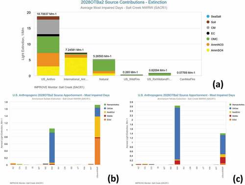
Salt Creek Wilderness Area (‘SACR’), New Mexico

Similar to LOST, SACR (Figure 9) is another example of a relatively isolated CIA that is significantly affected by emissions from oil and gas development. It also has one of the highest levels of future particle visibility impairment at 32.4 Mm⁻¹. U.S. anthropogenic emissions are primarily responsible for haze at SACR (18.7 Mm⁻¹), followed by international contributions (7.2 Mm⁻¹), the bulk of which is AmmSO4, and possibly originates from Mexican SO₂ sources given SACR’s location (Figure 9(a)). Two prominent sources of domestic AmmSO4 and AmmNO3 are evident: New Mexico oil and gas development (with a combined impact of 3.2 Mm⁻¹), and a mix of sectors from states outside of the WRAP region (Figures 9(b,c)).

Figure 9. Salt Creek Wilderness Area (‘SACR’; New Mexico) high-level source apportionment results (a) and low-level source apportionment results for (b) AmmSO4 and (c) AmmNO3 from anthropogenic sources.

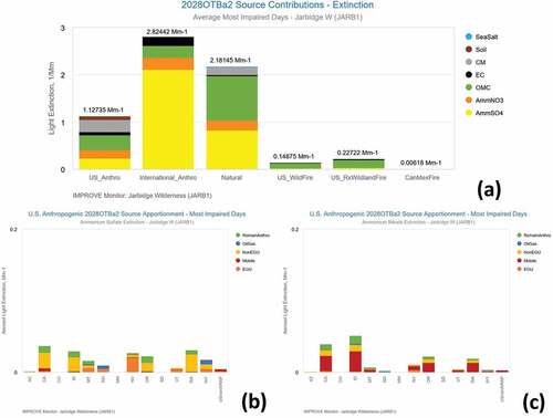
Jarbidge Wilderness Area (‘JARB’), Nevada

This remote wilderness, located in northeastern Nevada near the Idaho border, has the distinction of being the least impaired CIA in this set of examples, with an estimated future particle light extinction of 6.5 Mm⁻¹ (Figure 10). The U.S. anthropogenic contribution is relatively small at 1.1 Mm⁻¹, with the AmmSO4 and AmmNO3 impacts widely distributed among the WRAP region states (Figures 10(b,c)). International and natural sources play the dominant role at 2.8 and 2.2 Mm⁻¹, respectively.

Figure 10. Jarbidge Wilderness Area (‘JABR’; Nevada) high-level source apportionment results (a) and low-level source apportionment results for (b) AmmSO4 and (c) AmmNO3 from anthropogenic sources.

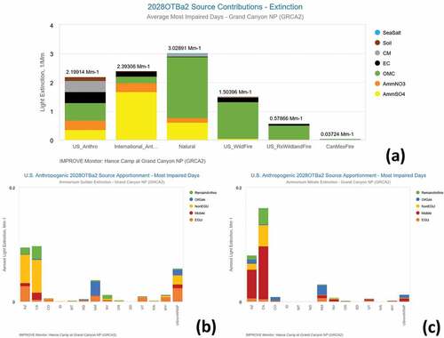
Grand Canyon National Park (‘GRCA’), Arizona

Like YELL, ROMO, and JARB, GRCA (Figure 11) is among the less hazy of the eight examples presented here, with an estimated future particle extinction of 9.7 Mm⁻¹. Organic matter carbon from fires and natural sources contributes approximately half of the estimated future particle impairment at 4.7 Mm⁻¹ (Figure 11(a)). AmmSO4 from international sources is 1.7 Mm⁻¹. Arizona, California, and New Mexico contribute the most to AmmSO4 and AmmNO3 impacts from U.S. anthropogenic sources.

Figure 11. Grand Canyon National Park (‘GRCA’; Arizona) high-level source apportionment results (a) and low-level source apportionment results for (b) AmmSO4 and (c) AmmNO3 from anthropogenic sources.

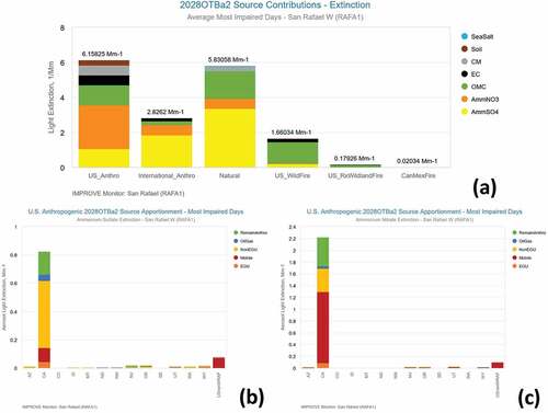
San Rafael Wilderness Area (‘RAFA’), California

The last example in this series is RAFA (Figure 12), located in southern California near the Pacific coast, and approximately 200 km northwest of Los Angeles. Estimated future particle impairment is 16.7 Mm⁻¹, with U.S. anthropogenic sources as the largest contributor at 6.2 Mm⁻¹. Natural sources are also prominent at 5.8 Mm⁻¹, and, like OLYM, a significant fraction is AmmSO4 at 3.4 Mm⁻¹. Almost all of the impairment from AmmSO4 and AmmNO3 is associated with U.S. anthropogenic sources (0.8 Mm⁻¹ and 2.2 Mm⁻¹, respectively), originating from SO₂ and NO_x emissions within California (Figures 12(b,c)).

Figure 12. San Rafael Wilderness Area (‘RAFA’; California) high-level source apportionment results (a) and low-level source apportionment results for (b) AmmSO4 and (c) AmmNO3 from anthropogenic sources.

The role of oil and gas emissions on future visibility estimates

A notable feature in the low-level source apportionment results is the significant impact of oil and gas activities on visibility at LOST and SACR, and to a lesser extent ROMO (Figures 7(b,c), 9 (b,c), and 8(b,c), respectively). Previous modeling studies have indicated the potential effects that oil and gas development in the WRAP region states could have on regional air quality, including worsening levels of ozone and haze-forming particles (Rodriguez, Barna, and Moore 2009; Thompson et al. 2017). The Bakken Air Quality Study (BAQS; Prenni et al., 2016) in North Dakota also illustrated the potential impacts from oil and gas emissions at regional CIAs. Contrary to the estimated emissions from other sectors, which generally decline in the future, oil and gas emissions can rise significantly within individual states (Table 1). For example, estimated future SO₂ and NO_x emissions in New Mexico increase by 7,546 and 12,437 ton/yr, respectively, as compared to the current 2014–2018 representative baseline emissions. These increases, along with oil and gas emissions in nearby Texas, are likely deteriorating future visibility estimates for SACR (Figure 9(b,c)). 2028 North Dakota SO₂ emissions associated with oil and gas activity increase by 5,812 ton/yr, but NOx emissions decline by 4,921 ton/yr, and emissions from this sector for Colorado remain relatively unchanged. Also notable in Table 1, and shown in Figures 2 and 3, are the considerable SO₂ and NO_x emissions from oil and gas basins within the WRAP region states, making this one of the largest contributing sectors to U.S. anthropogenic emissions in the western U.S.

Table 1. Estimated SO2 and NOx emissions (ton/yr) from oil and gas activity for North Dakota, New Mexico, and Colorado from the representative baseline (2014–2018, ‘RepBase2’) and future (2028, ‘2028otba2’) inventories.

	RepBase2	2028OTBa2	RepBase2	2028OTBa2
	SO2	SO2	NOx	NOx
	(ton/yr)	(ton/yr)	(ton/yr)	(ton/yr)
North Dakota
Oil and Gas – Point	5,814	5,814	5,179	5,179
Oil and Gas – Non-point	9,391	15,203	62,190	57,269
Total	15,205	21,017	67,369	62,448
Difference		5,812		-4,921
New Mexico
Oil and Gas – Point	8,641	11,937	31,244	43,652
Oil and Gas – Non-point	14,484	18,734	50,064	50,093
Total	23,125	30,671	81,308	93,745
Difference		7,546		12,437
Colorado
Oil and Gas – Point	514	478	17,226	14,677
Oil and Gas – Non-point	22	24	26,987	29,062
Total	536	502	44,213	43,739
Difference		−34		−474

Example application of using the modeled most impaired days (‘ModMID’)

There is an additional interpretation of the source apportionment estimates that can be invoked by using the modeled most impaired days (ModMID) as opposed to the conventional MID. The days in the ModMID are defined as the 20% of days with the highest simulated fraction of impairment due to U.S. anthropogenic emissions; a detailed discussion of its implementation can be found at WRAP (2021b). Although it is anticipated that state planners will employ the more conventional MID, the ModMID provides the ability to explicitly track the contribution of U.S. anthropogenic sources over all days within a calendar year, as opposed to an interpretation of the U.S. anthropogenic sources on every third day (corresponding to the frequency of IMPROVE sample collection). An example is shown by revisiting the high-level source apportionment results for RAFA (Figure 13). Immediately apparent is the reduction in natural and U.S. wildfire contributions using the results based on the ModMID estimate (Figure 13(b)) as compared to the conventional MID (Figure 13(a)), with impacts from natural emissions dropping from 5.8 Mm⁻¹ to 3.4 Mm⁻¹, and 1.7 Mm⁻¹ to 0.3 Mm⁻¹ for U.S. wildfires. As expected, the U.S. anthropogenic contribution rises, from 6.2 to 6.8 Mm⁻¹. There is also a modest increase in international contributions and U.S. prescribed wildland fires of approximately 0.2 Mm⁻¹ for both cases.

Figure 13. Example high level source apportionment results using (a) the 20% Most Impaired Days (‘MID’) and (b) the 20% Modeled Most Impaired Days (‘ModMID’) at San Rafael Wilderness Area (‘RAFA’).

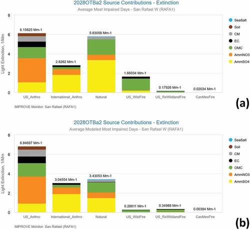
Although the MID metric is intended to limit the influence of episodic wildfires and dust storms on visibility tracking, it still struggles with the role of organic particles from fires and ammonium sulfate originating from dimethyl sulfide emissions from marine algae (this is especially evident at coastal CIAs when examining the contribution of AmmSO4 from natural sources, as illustrated at RAFA and also OLYM (Figure 5(a)). Even though the MID has been revised by EPA to emphasize the importance of AmmSO4 and AmmNO3, which are presumed to originate from manmade sources of SO₂ and NO_x, respectively, as a measurement-based approach it cannot distinguish between AmmSO4 and AmmNO3 that arise from domestic versus international emissions. The ModMID approach, however, explicitly resolves the days of most impairment by U.S. anthropogenic sources, since it relies on the CAMx source apportionment results and not an inference of the IMPROVE measurement. Of course, given 1) the inherent inaccuracies in the modeling platform, and 2) the two-out-of-three days that are missing from the IMPROVE measurement record, it can be difficult to reconcile the MID and ModMID approaches. Again, it is assumed that state planners will rely on the conventional MID approach for their RHR SIP development, but the ModMID analyses for CIAs in the western U.S. is available at the WRAP TSS for consideration.

Conclusion

Even in this small set of eight examples (summarized in Table 2), there is clearly a diversity of source apportionment estimates evident at the WRAP region CIAs. Perhaps one of the most obvious features from the results presented above is the relative contribution of U.S. anthropogenic emissions as compared to emissions from international anthropogenic sources, natural sources, and fires. Less than half of the estimated future impairment is from domestic sources (17% − 44%), except at SACR (58%). This is especially apparent at sites with lower levels of future visibility impairment, such as YELL, ROMO, JARB, and GRCA. These results are consistent with the EPA’s 2028 visibility projections (U.S. EPA 2019) at these same sites, even though the EPA CAMx modeling was focused on a different base year (2016 versus 2014 in this study).

Table 2. Summary of the high-level source apportionment results by emission categories for the eight example CIAs.

	U.S. Anthro		Int’l Anthro		Natural		U.S. Wildfire		U.S. Prescribed Fire		Can Mex Fire		Total
	(Mm-1)	(%)	(Mm-1)	(%)	(Mm-1)	(%)	(Mm-1)	(%)	(Mm-1)	(%)	(Mm-1)	(%)	(Mm-1)
OLYM	9.80	28.3%	6.72	19.4%	10.49	30.3%	6.90	19.9%	0.22	0.6%	0.50	1.4%	34.63
YELL	2.25	21.5%	2.31	22.1%	3.95	37.7%	1.41	13.5%	0.40	3.8%	0.15	1.4%	10.47
LOST	10.22	41.8%	9.64	39.4%	3.94	16.1%	0.09	0.4%	0.36	1.5%	0.20	0.8%	24.45
ROMO	4.35	44.4%	2.36	24.1%	2.52	25.7%	0.35	3.6%	0.18	1.8%	0.04	0.4%	9.80
SACR	18.71	57.7%	7.25	22.4%	5.27	16.3%	0.27	0.8%	0.82	2.5%	0.08	0.2%	32.40
JARB	1.13	17.3%	2.82	43.3%	2.18	33.4%	0.15	2.3%	0.23	3.5%	0.01	0.2%	6.52
GRCA	2.20	22.6%	2.39	24.5%	3.03	31.1%	1.50	15.4%	0.58	6.0%	0.04	0.4%	9.74
RAFA	6.16	36.9%	2.83	17.0%	5.83	35.0%	1.66	10.0%	0.18	1.1%	0.02	0.1%	16.68

Brewer et al. (2019) also examined simulated visibility impacts and the role of U.S. anthropogenic contributions, but for 2011 instead of 2028. With regard to AmmSO4 estimates at OLYM, YELL, ROMO, and GRCA, they found 19.5%, 29.5%, 62.5%, and 24.8% of the visibility impairment, respectively, was contributed by U.S. anthropogenic sources. In comparison, from this study, the high-level source apportionment estimates for U.S. anthropogenic AmmSO4 at these same sites is 12.2%, 13.3%, 29.0%, and 14.8%, respectively. Clearly these two analyses are not directly comparable, given that they represent different base year meteorology simulations, emission inventories, and boundary condition estimates. In particular, SO₂ and NO_x emissions from fossil fuel EGUs and mobile sources in the WRAP region states have declined dramatically in recent years (Center for the New Energy Economy 2019; Ramboll 2020b), and this trend is expected to continue. What this brief comparison suggests, and as shown by Figures 5(a)–12(a) for the AmmSO4 component of the international anthropogenic contribution, is that CIAs in the western U.S. will continue to be significantly affected by sources other than domestic anthropogenic sources. Additional evaluation of the global-scale model simulations that define the CAMx boundary conditions is warranted, given their influence on haze estimates in the western U.S.

Acknowledgement

The results of this paper were made possible by the air quality and emissions modeling team at Ramboll of Tejas Shah, Marco Rodriguez, Chao-Jung Chien and Pradeepa Vennam. The authors would also like to acknowledge Shawn McClure of Colorado State University who implemented the visualization of the modeling results on the WRAP Technical Support System. This paper does not reflect EPA policy, guidance or recommendations.

Disclosure statement

No potential conflict of interest was reported by the author(s).

Data availability statement

The data that support the findings of this study are openly available at the Western Regional Air Partnership’s Technical Support System (WRAP TSS):

http://views.cira.colostate.edu/tssv2/Express/ModelingTools.aspx

http://views.cira.colostate.edu/tssv2/Express/EmissionsTools.aspx

Additional information

Notes on contributors

Michael Barna

Michael Barna is a physical scientist with the Air Resources Division of the National Park Service. His work focuses on identifying emission sources that impact air quality at national parks and other sensitive ecosystems through the application of regional air quality models.

Ralph Morris

Ralph Morris is a Managing Principal at Ramboll Environment and Health. He has over 40 years of experience in the development and application of air quality models including as one of the leads in the development of the Comprehensive Air-quality Model with extensions (CAMx).

Patricia Brewer

Patricia Brewer worked for the National Park Service Air Resources Division in regional haze and acid deposition science and policy until retirement in 2019. From 2019-2021 she supported the Western Regional Air Partnership in delivery of regional haze modeling analyses for use in western states’ regional haze implementation plans.

Tom Moore

Tom Moore is the Technical Services Program manager for the State of Colorado’s Air Pollution Control Division in the Dept. of Public Health and the Environment. He previously worked for WESTAR/WRAP for more than 20 years, coordinating and managing the regional analyses and planning support for visibility, ozone, and other western U.S. regional programs and issues.

Gail Tonnesen

Gail Tonnesen is an air quality modeler at the EPA Region 8 office in Denver, CO.

Kevin Briggs

Kevin Briggs is the Regional Modeling and Emission Inventory Supervisor at the Colorado Department of Public Health and Environment-Air Pollution Control Division. He has been at the Colorado APCD for 33 years and leads the regional modeling and emission inventory development efforts for such projects as the State Implementation Plans.

References

- Air Sciences. 2020. Fire emission inventories for regional haze planning: methods and results. Air Sciences, Inc., Portland, Oregon. April. http://wrapair2.org/pdf/fswg_rhp_fire-ei_final_report_20200519_FINAL.PDF
- Aksoyoglu, S., G. Ciarelli, I. El-Haddad, U. Baltensperger, and A. S. H. Prévôt. 2017. Secondary inorganic aerosols in Europe: Sources and the significant influence of biogenic VOC emissions, especially on ammonium nitrate. Atmos. Chem. Phys. 17 (12):7757–73. doi:10.5194/acp-17-7757-2017.
- Bey, I., D. Jacob, R. Yantosca, J. Logan, B. Field, A. Fiore, Q. Li, H. Liu, L. Mickley, and M. Schultz. 2001, October 16. Global modeling of tropospheric chemistry with assimilated meteorology: model description and evaluation. J. Geophys. Res. Atmos. 106 (D19):23073–95. doi:10.1029/2001JD000807.
- Bowden, J., K. Talgo, and Z. Adelman. 2016. Western-State Air Quality Modeling Study (WAQS) – Weather Research Forecast 2014 Meteorological Model Application/Evaluation. University of North Carolina at Chapel Hill – Institute for the Environment. January 1. http://views.cira.colostate.edu/wiki/Attachments/Modeling/WAQS_2014_WRF_MPE_January2016.pdf
- Brewer, P., G. Tonnesen, R. Morris, T. Moore, U. Nopmongcol, and D. Miller. 2019. Air pollutant source characterization using the revised regional haze tracking metric and a photochemical grid model and implications for regional haze planning. J. Air Waste Manag. Assoc. 69 (3):373–90. doi:10.1080/10962247.2018.1537985.
- Center for the New Energy Economy. 2019. Analysis of EGU emissions for regional haze planning and ozone transport contribution, project report for WESTAR-WRAP, Final Report June 14, http://www.wrapair2.org/EGU.aspx
- Gantt, B., M. Beaver, B. Timin, and P. Lorang. 2018. Recommended metric for tracking visibility progress in the Regional Haze Rule. J. Air Waste Manag. Assoc. 68 (5):438–45. doi:10.1080/10962247.2018.1424058.
- Hand, J. L., B. A. Schichtel, W. C. Malm, and N. H. Frank. 2013. Spatial and temporal trends in PM2.5 organic and elemental carbon across the United States. Adv. Meteor. ID:367674. doi:10.1155/2013/367674.
- Hand, J. L., W. H. White, K. A. Gebhart, N. P. Hyslop, T. E. Gill, and B. A. Schichtel. 2016. Earlier onset of the spring dust season in the southwestern United States. Geophys. Res. Lett. 43 (8):4001–09. doi:10.1002/2016GL068519.
- Koo, B., G. Wilson, R. Morris, A. Dunker, and G. Yarwood. 2009. Comparison of source apportionment and sensitivity analysis in a particulate air quality model. Environ. Sci. Technol. 43 (17):6669–75. doi:10.1021/es9008129.
- Morris, R., G. Tonnesen, P. Brewer, and T. Moore. 2022. Assessment of progress toward regional haze rule visibility goals using United States anthropogenic emissions rate of progress, submitted to J. Air & Waste Manage.
- Pepe, N., G. Pirovano, A. Balzarini, A. Toppetti, G. M. Riva, F. Amato, and G. Lonati. 2019. Enhanced CAMx source apportionment analysis at an urban receptor in Milan based on source categories and emission regions. Atmos. Environ. X 2:100020. doi:10.1016/j.aeaoa.2019.100020.
- Pitchford, M., W. Malm, B. Schichtel, N. Kumar, D. Lowenthal, and J. Hand. 2007. Revised algorithm for estimating light extinction from IMPROVE particle speciation data. J. Air Waste Manag. Assoc. 57 (11):1326–36. doi:10.3155/1047-3289.57.11.1326.
- Prenni, A. J., D. E. Day, A. Evanoski-Cole, B. C. Sive, A. Hecobian, Y. Zhou, and B. A. Schichtel. 2016. Oil and gas impacts on air quality in federal lands in the Bakken region: An overview of the Bakken air quality study and first results. Atmos. Chem. Phys. 16 (3):1401–16. doi:http://dx.doi.org/10.5194/acp-16-1401-2016.
- Ramboll. 2018. Representativeness analysis of candidate modeling years for the Western U.S. http://www.wrapair2.org/pdf/WESTAR_RTOWG_Representativeness_final.pdf
- Ramboll. 2020a. User’s guide comprehensive air quality model with extensions, Version 7.1. https://camx-wp.azurewebsites.net/Files/CAMxUsersGuide_v7.10.pdf
- Ramboll. 2020b. Mobile source emissions inventory development for implementation in WRAP regional haze modeling. https://views.cira.colostate.edu/docs/wrap/mseipp/WRAP_MSEI_Summary_Memo_13Mar2020.pdf
- Rodriguez, M. A., M. G. Barna, and T. Moore. 2009. Regional impacts of oil and gas development on ozone formation in the Western United States. J. Air Waste Manag. Assoc. 59 (9):1111–18. doi:10.3155/1047-3289.59.9.1111.
- Skamarock, W. C., J. B. Klemp, J. Dudhia, D. O. Gill, D. M. Barker, M. G. Duda, X.-Y. Huang, W. Wang, and J. G. Powers, 2008: A description of the Advanced Research WRF Version 3. NCAR Technical Note 475. https://opensky.ucar.edu/islandora/object/technotes:500
- Solomon, P., D. Crumpler, J. Flanagan, R. Jayanty, E. Rickman, and C. McDade. 2014. U.S. National PM 2.5 chemical speciation monitoring networks—CSN and IMPROVE: Description of networks. J. Air Waste Manag. Assoc. 64 (12):1410–38. doi:10.1080/10962247.2014.956904.
- Thompson, T. M., D. Shepherd, A. Stacy, M. G. Barna, and B. A. Schichtel. 2017. Modeling to evaluate contribution of oil and gas emissions to air pollution. J. Air Waste Manag. Assoc. 67 (4):445–61. doi:10.1080/10962247.2016.1251508.
- U.S. EPA. 1999. Regional Haze Regulations, Final Rule. U.S. Environmental Protection Agency. 40 CFR Part 51. Federal Register/Vol. 64, No. 126/Thursday. Accessed July 1, 1999, pp. 35714–74. https://www.govinfo.gov/content/pkg/FR-1999-07-01/pdf/99-13941.pdf
- U.S. EPA. 2017. Protection of Visibility Amendments to Requirements for State Plans, Final Rule. U.S. Environmental Protection Agency. 40 CFR Parts 51 and 52. Federal Register/Vol. 82, No. 6/Tuesday, Accessed January 10, 2017, pp. 3078–129. https://www.govinfo.gov/content/pkg/FR-2017-01-10/pdf/2017-00268.pdf
- U.S. EPA. 2018. Technical Support Document (TSD): Preparation of emissions inventories for the Version 7.1 2014 emissions modeling platform for the national air toxics assessment. https://www.epa.gov/air-emissions-modeling/2014-version-71-technical-support-document-tsd
- U.S. EPA. 2019. Technical Support Document for EPA’s Updated 2028 Regional Haze Modeling. U.S. Environmental Protection Agency, Office of Air Quality Planning and Standards, Research Triangle Park, NC, September 19. https://www.epa.gov/sites/default/files/2019-10/documents/updated_2028_regional_haze_modeling-tsd-2019_0.pdf
- U.S. EPA. 2021. Technical Support Document (TSD): Preparation of emissions inventories for the 2016v1 North American emissions modeling platform. https://www.epa.gov/air-emissions-modeling/2016-version-1-technical-support-document
- WRAP. 2019. Western regional modeling and analysis platform – Initial 2014 platform development and shake-out. https://views.cira.colostate.edu/iwdw/docs/waqs_2014v1_shakeout_study.aspx
- WRAP. 2020a. Weighted Emissions Potential (WEP) and Area of Influence (AOI) Analyses, https://views.cira.colostate.edu/docs/iwdw/platformdocs/WRAP_2014/Run_Spec_WRAP_2014_Task6-2_WEP-AOI-SA_v5.pdf
- WRAP. 2020b. Dynamic evaluation – 2002 CAMx simulation and analysis, run specification sheet. Western regional air partnership and Ramboll. February 24. https://views.cira.colostate.edu/docs/iwdw/platformdocs/WRAP_2014/Run_Spec_WRAP_2014_Task3_Dynamic-Evaluation_v1.pdf
- WRAP. 2020c. WRAP/WAQS 2014v2 modeling platform description and western region performance evaluation. http://views.cira.colostate.edu/iwdw/docs/WRAP_WAQS_2014v2_MPE.aspx
- WRAP. 2020d. High-Level and low-level source apportionment modeling using the Repbase2 and 2028otba2 Emission Scenarios. https://views.cira.colostate.edu/docs/iwdw/platformdocs/WRAP_2014/SourceApportionmentSpecifications_WRAP_RepBase2_and_2028OTBa2_High-LevelPMandO3_and_Low-Level_PM_andOptionalO3_Sept29_2020.pdf
- WRAP. 2021a. Future Fire Sensitivity Simulations. https://views.cira.colostate.edu/docs/iwdw/platformdocs/WRAP_2014/Run_Spec_WRAP_Future_Fire_Sensitivities_August4_2021_final.pdf
- WRAP. 2021b. WRAP technical support system for regional haze planning: emissions methods, results, and references, https://views.cira.colostate.edu/tssv2/Docs/WRAP_TSS_emissions_reference_final_20210930.pdf
- WRAP. 2021c. WRAP technical support system for regional haze planning: modeling methods, results, and references, https://views.cira.colostate.edu/tssv2/Docs/WRAP_TSS_modeling_reference_final_20210930.pdf