Characterization of the short-term temporal variability of road dust chemical mixtures and meteorological profiles in a near-road urban site in British Columbia

ABSTRACT

Springtime road dust is a common air quality concern for northern latitudes communities. Traction material, brake wear, tire wear, and other particles entrained in snow during winter become re-suspended into the air as the snow melts. Characterization of within-season variability of road dust composition and weather conditions is critical to understanding its acute health impacts. Sixty 24-hour samples of PM₁₀ were collected with a high-volume sampler at a near-road site in Prince George, British Columbia. Near-road samples were collected intermittently in winter and daily in spring. All samples were analyzed for 18 trace elements. We used data from a nearby regulatory monitor to estimate daily coarse fraction (PM_10–2.5). Proportion of PM_10–2.5 in PM₁₀ was used to classify days as high or low road dust based on a threshold of 65% PM_10–2.5. We identified clusters of near-road samples based on weather parameters and PM₁₀ components using Bayesian profile regression (BPR). Twenty-one near-road PM₁₀ samples were classified as high road dust days and 34 as low road dust days. Concentrations of total trace elements and specific trace elements were significantly higher on high road dust days (aluminum, chromium, iron, lead, tin, vanadium, and zinc). High road dust days also had low relative humidity and precipitation and higher temperature and air pressure. We identified five clusters of near-road PM₁₀ mixtures that suggested an interaction between temperature and humidity for road dust impacts. Samples from a near-road site indicated days highly affected by springtime road dust are distinct from other days based on particulate mixtures and meteorological factors. Higher loading of trace element mixtures in PM₁₀ on high road dust days has important implications for acute toxicity of road dust. Relationships between road dust and weather may facilitate further research into health effects of road dust as the climate changes.

Implications: Non-tailpipe emissions driven by springtime road dust in northern latitude communities is increasing in importance for air pollution control and improving our understanding of the health effects of chemical mixtures from particulate matter exposure. High-volume samples from a near-road site indicated that days affected by springtime road dust are substantively different from other days with respect to particulate matter mixture composition and meteorological drivers. The high load of trace elements in PM₁₀ on high road dust days has important implications for the acute toxicity of inhaled air and subsequent health effects. The complex relationships between road dust and weather identified in this study may facilitate further research on the health effects of chemical mixtures related to road dust while also highlighting potential changes in this unique form of air pollution as the climate changes.

Introduction

Ambient particulate matter (PM) air pollution is a ubiquitous environmental exposure shown to have a causal link with multiple adverse health outcomes, making it a significant contributor to the global burden of disease (Sang et al. 2022; Tong 2019; Wu et al. 2021). On-road emissions are one driver of PM-related disease burden. In the higher-income countries of North America, on-road PM ranks as the second largest contributor to overall PM emissions (11.7%) (McDuffie et al. 2021). Furthermore, in the United States alone, approximately 20,000 annual deaths have been attributed to transportation-related PM emissions (Choma et al. 2021).

Particle size distribution and mixture composition contribute to the public health risks associated with roadway PM air pollution. PM with an aerodynamic diameter <10 µm (PM₁₀) is classified into different size fractions, including the coarse size fraction between 2.5 and 10 µm in aerodynamic diameter (PM_10–2.5) and the fine size fraction <2.5 µm in aerodynamic diameter (PM_2.5). Although it is well-documented that PM_2.5 is a leading cause of global morbidity and mortality (Tong 2019), the body of evidence on the health effects of PM_10–2.5 is smaller. The epidemiologic evidence for PM_10–2.5 is less clear due to fewer studies compared with PM_2.5 and inconsistent findings in the literature (Adar et al. 2014; Health Canada 2016).

Emissions from roadway traffic are a major source of PM in cities (Mukherjee et al. 2020), comprising exhaust (tailpipe) and non-exhaust sources. In urban environments, PM_10–2.5 can serve as a signature of non-exhaust roadway emissions due to its origin from different mechanical processes. In contrast, PM_2.5 is a signature of exhaust emissions related to combustion processes and gas-to-particle conversions in the atmosphere. PM exhaust emissions have decreased due to decades of targeted air pollution policy and management decisions (Stojiljkovic et al. 2019; Winkler et al. 2018). On the other hand, non-exhaust emissions have been relatively neglected, and their contribution to overall air quality is increasing. For example, a PM emissions inventory study for Europe estimated that the contribution to PM₁₀ from non-exhaust emissions relative to tailpipe emissions increased from 32% in 2000 to 63% in 2017. Similarly, the relative contribution to PM_2.5 from non-exhaust emissions increased from 18% in 2000 to 46% in 2017 (EEA 2022).

A recent report (OECD 2020) by the Organization for Economic Co-operation and Development (OECD) confirms the growing importance of non-exhaust emissions, estimating that a majority of PM from on-road traffic will come from non-exhaust sources by 2035. This report suggests that the onset of electric vehicles could worsen the road dust problem. For instance, they estimate that electric cars emit 3–8% more non-exhaust PM_2.5 than conventional vehicles (OECD 2020). Understanding roadway non-exhaust PM is therefore necessary for air quality management and the protection of public health.

Source apportionment studies have shown that non-exhaust PM₁₀ originates from road traction material (e.g., sand and salt), wear of road surfaces, brakes, and tires. These particles can accumulate on road surfaces over time and then become suspended as road dust under certain weather conditions (Stojiljkovic et al. 2019). Suspension of road dust during springtime thawing periods has long been a source of PM₁₀ exceedances in many northern latitude regions, including provinces of Canada (Graham et al. 2005). In addition, some studies conducted in northern latitudes show that PM_10–2.5 constitutes a higher proportion (relative to PM_2.5) of the mass concentration of PM₁₀ during springtime (Ferm and Sjöberg 2015; Soleimanian et al. 2019; Zhang et al. 2022). The accumulation of PM in snow and on road surfaces during winter, followed by springtime thawing, can contribute to the suspension of large amounts of road dust by passing vehicles, particularly during dry weather episodes.

The elemental composition of roadway PM emissions is a critical public health consideration. Harmful trace metals (e.g., cadmium, copper, lead, etc.) occur in greater abundance in the respirable PM range in urban environments (Moreno et al. 2009; Samara and Voutsa 2005; Shah et al. 2006; Xie et al. 2019; Zereini et al. 2005). Mass fractions of trace elements that are signatures of non-exhaust traffic emissions in PM₁₀ and PM_2.5 road dust also decrease with increasing distance from roadways (Huang et al. 2021). With the influence of meteorological factors on roadway dust episodes, PM₁₀ chemical mixtures may also vary within seasons, such as springtime. Therefore, chemical mixtures of urban road dust and PM_10, and thus toxicity, may vary over short time scales (i.e., days). However, most studies that assessed temporal variability of road dust PM mixture composition have investigated trends over more extended periods (i.e., months or seasons).

From a health effects standpoint, within-season variability in PM mixture composition is relevant for acute health effects, including explaining daily variation in morbidity and mortality (Achilleos et al. 2017; Atkinson et al. 2016; Basagaña et al. 2015). A recent time-series study conducted in England applied cluster analysis to daily metal concentrations in PM₁₀ and PM_2.5. The research identified clusters of metals in PM₁₀ mixtures that were characteristic of road dust and were associated with higher daily cardiovascular and respiratory mortality (Lavigne et al. 2020). Another time series study conducted in British Columbia (BC), Canada, showed that PM_10–2.5 was associated with higher-than-expected daily mortality during the spring (Hong et al. 2017). In contrast, springtime PM_2.5 was not associated with daily mortality. These studies underscore the need to evaluate the short-term, within-season variability of road dust composition and the possible drivers of composition variability.

We conducted this study in the city of Prince George, located in the central interior of the Canadian province of BC. It focuses on the springtime road dust season with the aims to (1) measure the daily contributions of trace elements (including heavy metals) to near-road PM₁₀; (2) explore the within-season temporal trends of PM_10–2.5 and PM_2.5 in PM₁₀; (3) classify days with high levels of springtime road dust based on a threshold of the proportion of PM_10–2.5 in PM₁₀, and (4) characterize the chemical-weather profiles of days with high levels of road dust. These aims will allow us to investigate our hypotheses that: (a) PM₁₀ is characterized by high within-season variability of chemical mixture composition; (b) chemical mixtures vary significantly between high road dust days compared with low road dust days; and (c) PM₁₀ chemical mixtures cluster together with distinct meteorological profiles. Thus, we provide insights into the daily variability of road dust chemical mixture composition in springtime and its potential time-varying acute human toxicity. We also incorporate multivariable regression and cluster analyses to provide further insights into distinct temporal weather-multi-pollutant patterns and their complex relationships with springtime road dust.

Materials and methods

Site description

Prince George is the largest city in northern BC, with a population of approximately 90,000. Much of the city is in a bowl-shaped river valley at the intersection of two major highways, the primary trucking routes through the BC interior. A large rail yard also services local resource extraction industries and facilitates the movement of goods throughout BC. Such contextual elements have contributed to exceedances of Canadian air quality standards in the past (BC MOE 2016). The primary sources of PM_2.5 in the region include industry, residential wood heating, motor vehicles, rail traffic, open burning, and wildfires. The primary sources of PM_10–2.5 include winter traction material, dust from unpaved roads and surfaces, the rail yard, and emissions from construction and resource-based industries. Temperature inversions in the wintertime play a key role in episodes of poor air quality. Resuspension of road dust plays a key role in springtime when substantial snowmelt exposes materials entrained in the snow (BC MOE 2016). Sampling was conducted in Prince George because it is near the University of Northern British Columbia, has a regulatory air quality monitoring station, and episodes of springtime road dust have been well-documented.

Data collection and analysis

Air sampling

A high-volume air sampler (TISCH TE- 5000; TISCH Environmental, Cleves, OH) with a PM₁₀ inlet was located at a near-road site in downtown Prince George (Figure 1) to collect 24-hour PM₁₀ (denoted PM_10-HiVol throughout for clarity) samples. The sampler was placed on a rooftop at approximately 10.5 m above ground level (581.5 m above sea level). This location is next to part of the major highway corridors and the train yard. PM_10-HiVol was measured at the near-road site to help elucidate the trace elements in road dust (Samara and Voutsa 2005). We first conducted intermittent air sampling during the wintertime. From 26 January 2021 to 17 March 2021, 24-hour samples were collected on Tuesdays and Thursdays, from 09:00 to 09:00 the following day. Continuous sampling was not possible during this period due to COVID-19 restrictions at the building. However, continuous daily air sampling was conducted during the springtime when road dust episodes are most frequent. From 22 March 2021 to 09 May 2021, 24-hour samples were collected every day from 09:30 to 09:00 the following day. The intermittent sampling period provided a comparator to distinguish low road dust days in wintertime from high road dust days in the springtime.

Figure 1. Map of study area in Prince George, British Columbia and study sites including the near-road site, the National Ambient Pollution Surveillance (NAPS) site, and the Environment and Climate Change Canada (ECCC) weather station. The inset map highlights (red box) the location of Prince George in the BC interior region.

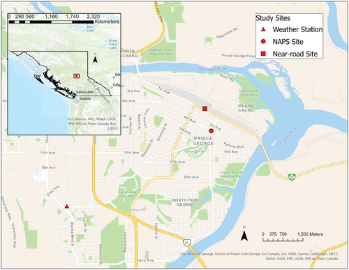
The near-road PM_10-HiVol air samples were collected on 8“x 10” Whatman QM-A quartz microfiber filters at an average flow rate of 1.71 m³/min. The flow rate was calibrated monthly using a variable orifice (K = 11.04) and corrected to ambient temperature and pressure. Filters were installed no more than 24 hours before sampling and were collected within 24 hours of the end of the sampling period. Filter samples were transported to the lab in sealed envelopes and stored at ≤2°C until further analysis.

We supplemented data from the high-volume sampler with data from a National Ambient Pollution Surveillance (NAPS) regulatory air quality monitoring site close to the near-road site (~500 meters away, Figure 1). The NAPS site has a continuous PM_2.5 beta attenuation monitor (BAM) and a PM₁₀ tapered element oscillating microbalance (TEOM). We ascertained PM_10–2.5 at the NAPS station by subtracting daily average concentrations of PM_2.5 from PM₁₀, calculated from 09:00 to 08:59 to correspond with the near-road samples.

Laboratory trace element measurement

We assessed the mass concentration and performed chemical analyses on PM_10-HiVol samples. Filters were weighed before and after sampling and equilibrated at 21°C ±2°C and 32% ± 2% relative humidity for a minimum of 24 hours before weighing. Filters were weighed in triplicate, and the final weighing (post-sampling) occurred within 30 days of their initial weighing (pre-sampling). After the final gravimetric analysis, each collected filter sample underwent extractions for subsequent chemical analysis for 18 trace elements (Table S1, Supplementary Information).

We used acid digestions for trace element extraction, adapted from the NIOSH 7303 method. Sample extracts were measured for elements using Agilent 5100 Inductively Couple Plasma Optical Emission Spectroscopy (ICP-OES). The minimum detection limit (MDL) for trace elements ranged from 0.1572 ng/m³ to 50.41 ng/m³ (detailed in Table S1, Supplemental Materials). While we detected trace elements in PM_10-HiVol for a majority of filter samples, three elements had more than 75% of values less than the detection level. We removed these low-detection elements from the computation of summary statistics of trace elements. All other filter samples with trace elements at sufficient detection frequencies were imputed using LOD/sqrt(2) if the samples was below the detection limit (Richardson and Ciampi 2003).

Meteorological data

We obtained historical hourly measurements of meteorological parameters from the Environment and Climate Change Canada (ECCC) online database (ECCC 2022). We downloaded data for the weather station in Prince George, nearest to the two air monitoring sites (Figure 1). The ECCC weather station is approximately 3.8 km and 3.6 km from the near-road and NAPS sites, respectively. Specific weather parameters included in the analysis are wind speed, wind direction, temperature, pressure, precipitation, and relative humidity. Hourly values for each parameter were averaged to daily values from 09:00 to 08:59 and linked with air monitoring data by date.

Data analysis

Identification of road dust days

Characterizing the composition of springtime road dust was the primary motivation for this study. Therefore, we developed an approach to distinguish between days when the ambient PM₁₀ was predominantly road dust (i.e., high road dust days) versus days when the PM₁₀ was not predominantly road dust (i.e., low road dust days). Because most non-exhaust PM emissions are in the coarse fraction (Fussell et al. 2022), we used the proportion of PM_10–2.5 in PM₁₀ at the NAPS monitoring site as a surrogate for road dust. We established a threshold of 65% to indicate high road dust days (Kuhns, Etyemezian, and Shinbein 2008), which in our study was the 75^th percentile value or greater for all measurement dates.

Preliminary analyses

Hourly mass concentrations of PM₁₀ and PM_2.5 at the NAPS site were aggregated to daily mean values from 09:00 to 08:59 to correspond with the daily PM_10-HiVol samples at the near-road site. We computed summary statistics, distributions, and between-variable correlations (Pearson’s or Spearman’s Rho) for all study variables. For specific trace elements, summary statistics and correlations were only computed for those with sufficient detection (≥25% of samples above LOD). All time-varying variables were visualized as daily time series and scatter plots to evaluate their temporal patterns and correlations between the different daily PM metrics (PM_10-HiVol, PM₁₀, PM_2.5, PM_10–2.5) and trace elements measured in the PM_10-HiVol samples. Linear and generalized linear regression models were fit to test adjusted associations between study variables and the different PM metrics, including the associations with the daily road dust classification and the sum of trace elements. All analyses were performed using R (version 4.2.1) (R Core Team 2022).

Bayesian profile regression

In addition to the preliminary analyses, we also performed a semi-parametric cluster analysis known as Bayesian Profile Regression (BPR) (Molitor et al. 2010). Previous studies have demonstrated that BPR facilitates the identification of clustered pollutant profiles that can be mapped to visualize spatial patterns (Coker et al. 2016, 2018; Hoover et al. 2018; Molitor et al. 2016). This study extends the previous work by exploring the temporal pattern of pollutant profiles (Lavigne et al. 2020) and combining the multi-pollutant data with relevant weather parameters of interest. Hence, with BPR, we can identify multi-pollutant-weather profiles through cluster membership. BPR also allows us to regress these multi-pollutant-weather profiles against an outcome of interest, such as the binary (low or high) road dust day classification. Because BPR uses Markov chain Monte Carlo (MCMC) methods, we can characterize the uncertainty of the joint distribution of the pollutant profiles. BPR also includes an option for variable selection to help identify which covariates of interest (e.g., trace elements and weather parameters) are driving the observed clustering (Liverani et al. 2015; Molitor et al. 2010; Papathomas et al. 2010).

In this application of BPR, we fit the concentrations of PM_10-HiVol and each trace element analyte and the levels of all weather patterns as covariates for clustering. Using logistic regression, the modeled response variable for BPR analysis was the binary indicator of road dust days, fit as a Bernoulli distribution (0 = low road dust; 1 = high road dust). These distributions of the pollutant covariates were highly skewed, so they were re-classified into quantiles prior to fitting BPR, and the quantiles were fit in BPR as discrete random variables. All weather parameters were fit as continuous variables in their original form. Our interpretation of the BPR analysis focuses on the joint levels of covariates within a cluster and the modeled association for each cluster with the road dust day classification. BPR was implemented using the PReMiuM package (version 3.2.7) (Liverani et al. 2015) in R.

Results and discussion

Particulate matter measurements

Sixty (60) 24-hr PM_10-HiVol air samples were collected at the near-road site between 26 January 2021 and 09 May 2021. Of these, 58 were valid. The sampled PM_10-HiVol daily average (standard deviation) concentration was 24.9 (17.0) µg/m³ (Table 1). Daily PM_10-HiVol concentrations varied markedly over the study period (Figure 1). At the NAPS station, the average concentrations of PM₁₀, PM_2.5, and PM_10–2.5 were 15.9 µg/m³ (11.1), 6.9 (4.2), and 8.9 (9.2), respectively (Table 1), with each PM fraction showing marked temporal variation throughout the study period (Figure 2). The fine PM_2.5 fraction dominated PM₁₀ in winter, while the coarse PM_10–2.5 dominated PM₁₀ in the spring (Figure 2).

Figure 2. Time series plot of daily PM_10-HiVol mass concentrations collected at the near-road site during the 2021 study period. The pink bars are days classified as high road dust (i.e., PM_10–2.5 more than ≥65% of PM₁₀ at NAPS site) and green bars are days classified as low road dust. Blue bars are considered unclassified (n = 3 days) due to a lack of PM_10–2.5 measurements on those three days.

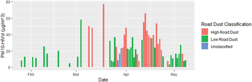
Figure 3. Time series plot of daily mass concentrations of PM₁₀ (grey bars), PM_2.5 (blue line), and PM_10–2.5 (red line) measured at the National Ambient Pollution Surveillance (NAPS) site during the 2021 study period.

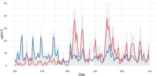
Table 1. Statistical summaries of PM concentrations (in µg/m³) measured at the near-road site (top row) and the National Ambient Pollutant Surveillance (NAPS) regulatory monitoring site in Prince George, British Columbia, between 26 January and 09 May 2021.

PM Metric	Mean	SD	Q1	Median	Q3
Near-road site
PM10-HiVol, n = 58	24.9	17.0	12.0	21.8	35.8
NAPS site
PM10, n = 102	15.9	11.1	8.6	11.3	20.0
PM2.5, n = 104	6.9	4.2	4.2	6.1	8.2
PM10–2.5, n = 102	8.9	9.2	2.3	5.7	12.7
Proportion PM10 from PM10–2.5, n = 102	0.47	0.24	0.25	0.50	0.67
Proportion PM10 from PM2.5, n = 102	0.53	0.24	0.33	0.50	0.75

SD = standard deviation; Q1 = 25^th percentile; Q3 = 75^th percentile.

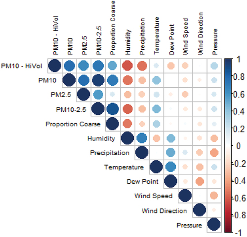
The measured PM_10-HiVol concentrations were significantly higher at the near-road site compared with PM₁₀ measured at the NAPS site (p < .001) when matching on measurement dates. Correlations between daily PM_10-HiVol and PM₁₀, PM_2.5, and PM_10–2.5 obtained from the NAPS site ranged from 0.63 to 0.76 (Figure 4). The strongest correlations between the meteorological variables and the different PM metrics from both sites were for relative humidity, precipitation, and temperature. Correlations with the PM metrics were generally negative for humidity, precipitation, and wind speed and positive for temperature. Relative humidity showed the most consistent correlations with the different PM metrics, particularly for the proportion PM_10–2.5 in PM₁₀ and concentrations of PM₁₀ and PM_10–2.5 at the NAPS site and PM_10-HiVol at the near-road site (Figure 4).

Figure 4. Between-variable Spearman’s correlations for different daily PM metrics and daily meteorological parameters. The PM metrics include high volume PM₁₀ samples from the near-road site (PM_10-HiVol), and PM₁₀ and PM_2.5 from the National Ambient Pollution Surveillance (NAPS) site, coarse fraction (PM_10–2.5) from the NAPS site, and the proportion of PM₁₀ that was PM_10–2.5. The relative size of the dots relate to the level of statistical significance of the correlation.

Multiple linear regression models using the meteorological variables explained a significant amount of variability of the different PM metrics, particularly for PM_10–2.5 concentration (R² = 0.39) and proportion PM_10–2.5 (R² = 0.53) at the NAPS site, and for PM_10-HiVol (R² = 0.40) concentrations at the near-road site. Models for PM₁₀ (R² = 0.30) and PM_2.5 (R² = 0.23) concentrations at the NAPS site were less predictive (Table S2, Supplemental Materials). After adjustment for all meteorological parameters, relative humidity resulted in significant negative linear relationships with PM_10-HiVol concentrations at the near-road site, as well as for PM₁₀ and PM_10–2.5 concentrations and PM_10–2.5 proportion at the NAPS site (Table S2, Supplementary Materials). After adjustment, wind speed was negatively associated with all PM metrics except for the proportion of PM_10–2.5 in PM₁₀. Temperature only resulted in a significant positive linear relationship with PM_10–2.5 concentration and proportion of PM_10–2.5 in PM₁₀ at the NAPS site.

At the NAPS site, PM_10–2.5 comprised a lower proportion (mean = 47%) of PM₁₀ overall compared with PM_2.5 (mean = 53%) during the study period. The relative daily abundance of PM_2.5 and PM_10–2.5 did vary significantly throughout the study period (Figure S1a, Supplemental Material). For example, the median of daily PM_2.5 comprised 86% and 78% of PM₁₀ in January and February. Conversely, the median PM_10–2.5 comprised 65% of PM₁₀ in March and April and 57% in May (Figure S1b). Analysis of variance (ANOVA) and Kolmogorov-Smirnov tests confirmed the significant (p < 0.0001) variation of the coarse fraction by month.

Trace element composition of PM₁₀

Most trace elements were detected in more than 50% of the PM_10-HiVol samples, except for arsenic (0%), mercury (0%), and antimony (12%). Average daily mass concentrations of all trace elements in PM_10-HiVol ranged from 0.05 to 615 ng/m³ (Table 2) and were skewed (Figure 5a) and highly variable during the study period (Figure 5b). The trace elemental composition of PM_10-HiVol by mass reached over 15% on multiple days and was likewise highly variable during the study period.

Figure 5. Daily sum concentrations of trace elements in PM_10-HiVol presented as (a) boxplots and (b) a time series.

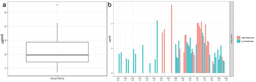
Table 2. Summary statistics for trace elements (ng/m3) measured in PM_10-HiVol measured at the near-road site.

Trace Elements	Median (IQR)*	% Detected in PM10-HiVol
Aluminum (Al), n = 57	226 (103, 466)	100
*Arsenic (As), n = 57	-	0
Barium (Ba), n = 57	8.3 (4.9, 12.8)	100
Cadmium (Cd), n = 57	0.05 (0.04, 0.0743)	51
Cobalt (Co), n = 57	0.24 (0.12, 0.50)	65
Copper (Cu), n = 57	481 (406, 665)	100
Chromium (Cr), n = 53	1.71 (1.10, 2.94)	100
Iron (Fe), n = 57	615 (318, 1,222)	100
Lead (Pb), n = 57	0.95 (0.58, 1.39)	70
Manganese (Mn), n = 57	14 (8, 28)	100
*Mercury (Hg), n = 57	-	0
Molybdenum (Mo), n = 57	34 (23, 41)	100
Nickel (Ni), n = 53	1.11 (0.68, 2.03)	100
Tin (Sn), n = 57	0.35 (0.28, 0.49)	62
Sulfur (S), n = 57	383 (216, 548)	100
*Antimony (Sb), n = 57	-	12
Vanadium (V), n = 57	0.87 (0.41, 2.15)	98
Zinc (Zn), n = 57	18 (13, 26)	100

IQR = Interquartile Range.

*Summary statistics not available for these elements due to their low detection in filter samples (<25%).

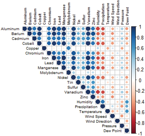
Overall, trace elements were highly correlated (Figure 6), indicating shared sources in the local environment. A few trace elements (e.g., copper, molybdenum, and sulfur) were weakly correlated with most other trace elements, suggesting these constituents had little overlap for shared sources in the local environment. Some of the more toxic metals with high detection, including chromium, lead, and cadmium, were correlated (Spearman range = 0.57, 0.75), suggesting a common source such as brake wear in non-exhaust road dust (Adamiec, Jarosz-Krzemińska, and Wieszała 2016; Celo, Yassine, and Dabek-Zlotorzynska 2021). Most trace elements had consistent correlations with weather parameters, generally similar to the relationships between the PM metrics and weather. Humidity, precipitation, and wind speed were negatively correlated with most trace elements. Days with a higher proportion of PM_10–2.5 in PM₁₀ at the NAPS site were also significantly correlated with higher total (summed) mass concentration of trace elements detected at the near-road site (spearman’s correlation = 0.37, p = .007).

Figure 6. Spearman’s correlations between trace elements and meteorological parameters. The relative size of the dots relate to the level of statistical significance of the correlation.

Characterization of road dust days

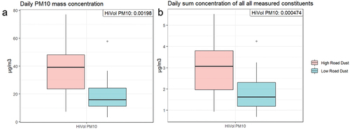
During the study period, 30.6% of days (31 days) during the study period were classified as high road dust days based on the proportion of PM_10–2.5 in PM₁₀ (≥65%) at the NAPS site. We had valid PM_10-HiVol samples on 55 of the 60 sampling days at the near-road site. Of these valid near-road PM_10-HiVol samples, 21 were collected on days with a high road dust classification and 34 were collected on days with a low road dust classification. Average daily mass concentrations of PM_10-HiVol were significantly elevated on high road dust compared with low road dust days (Figure 7a). The total mass concentration of trace elements was similarly elevated on high road dust days (Figure 7b). Concentrations for each trace element, except for copper, sulfur, and tin, were significantly elevated on high road dust days (Figure 7a,b). These analyses confirm that PM_10–2.5 (i.e., our surrogate for road dust) is associated with higher PM_10-HiVol concentrations and higher trace element composition at the near-road site.

Figure 7. Boxplots comparing the mass concentrations of PM_10-HiVol for high road dust days (pink) and low road dust days (light blue) at the near-road site (a), and the summed trace element mass concentrations measured in PM_10-HiVol samples (b). Kolmogorov-Smirnov tests indicate that the concentrations were significantly different by road dust classification (p-values in the upper right-hand corner of each boxplot) for each PM metric shown.

At the NAPS site, we also found that high road dust days were more common on weekdays than on weekends. PM_10–2.5 was also significantly elevated on weekdays compared with weekends (p < 0.05). The median proportion of PM_10–2.5 in PM₁₀ was higher on weekdays (57%) than on weekends (46%). In contrast, PM_2.5 was lower on weekdays compared with weekends. Thus, days with higher levels of PM_10–2.5 and road dust are associated with weekdays, when vehicle traffic and other anthropogenic activities are more prevalent than on weekend days (Jones, Yin, and Harrison 2008; Morawska et al. 2002).

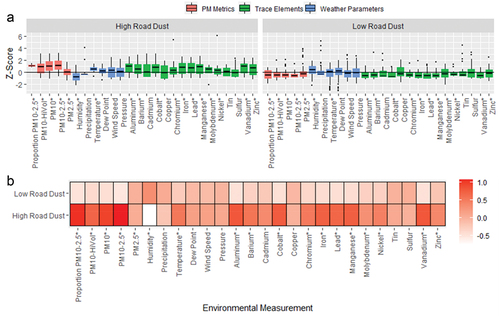
Only humidity and temperature differed significantly between high and low road dust days (Figure 8a,b); on days with high road dust humidity was lower and temperature was higher. Of all weather parameters, relative humidity was most strongly associated with road dust classification, with a mean humidity value of 51.2% on high road dust days compared with a mean humidity value of 66.1% on low road dust days. Temperature and precipitation were also significantly (p < 0.05) associated with the road dust classification, but the association was weaker. Polar plots integrating wind direction and wind speed did, however, suggest these as important meteorological drivers of PM levels, particularly for heavy metals in PM₁₀ at the near-road site and for PM_10–2.5 at the NAPS site (see Figure S2 in the Supplemental Materials).

Figure 8. Comparison of the PM metrics, weather parameters, and trace elements between days classified as high and low road dust. Values are displayed as (a) boxplots of Z-scores and (b) a heat map of average Z-scores. Z-scores are displayed to ensure values are on the same scale (and thus more comparable). Variables with * indicate statistically significant (p < 0.05) difference between high road dust versus low road dust days.

Bayesian profile regression (BPR) resulted in five clusters of multipollutant-weather profiles (Figure 9). The BPR variable selection indicates that all trace elements contributed to the observed clustering pattern except copper and sulfur, and all the weather parameters contributed to the clustering. A complete summary of the posterior distributions of pollutant-weather profiles from the full MCMC output is provided in the Supplementary Materials (Figure S3, Supplemental Material). The proportion of high road dust days and percent PM_10–2.5 in PM₁₀ varied significantly between clusters (Figure 9 and Table 3).

Figure 9. Boxplots (b) and heat map (a) of the multi-pollutant-weather profiles for each cluster from the Bayesian profile regression analysis. Z-scores were calculated for each covariate to put all variables on comparable scales. Covariates with an asterisk (*) beside their name indicate that the covariate levels varied significantly between clusters. Cluster 4 (C4) is the only profile with significantly elevated trace metals and PM metrics.

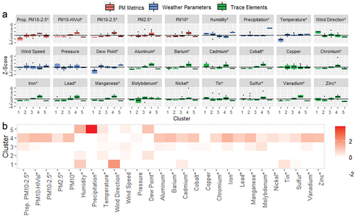
Table 3. Summaries of select study covariates stratified by clusters obtained from Bayesian profile regression. All covariates can be found in the supplemental information (Table S3).

Characteristic	1, N = 5^1	2, N = 20^1	3, N = 15^1	4, N = 14^1	5, N = 3^1	p-value^2
High Road Dust Day	0 (0%)	4 (20%)	4 (27%)	13 (93%)	1 (33%)	<0.001
Proportion PM10–2.5 in PM10	0.22 (0.04, 0.27)	0.53 (0.36, 0.62)	0.62 (0.48, 0.65)	0.75 (0.71, 0.76)	0.47 (0.34, 0.60)	<0.001
PM10-HiVol (mg/m^3)	13 (12, 16)	13 (10, 16)	27 (23, 34)	48 (39, 55)	7 (5, 8)	<0.001

¹Range; Median (IQR); n (%).

²Kruskal-Wallis rank sum test; Fisher’s exact test.

Relative to the population average daily levels for each pollutant, cluster 4 (C4) has days with significantly elevated levels for PM_10–2.5 (Figure 9). For C4, the median proportion of PM_10–2.5 in PM₁₀ was 75%, and 13 of the 14 days (93%) in C4 are days with high road dust (Table 3). Except for copper, molybdenum, and sulfur, levels for each trace metal were highest in C4 days compared with all other clusters and were significantly elevated compared to the baseline average levels (see Table S3, Supplemental Materials). High metal concentrations in C4 days suggest the highest potential for airborne inhalation toxicity would occur on these days.

In addition to its distinct elevated multi-pollutant PM₁₀ mixture, C4 also had a distinct weather profile. Compared with all the other clusters, C4 days had the lowest humidity (47%), the lowest wind speed (3.98 km/h), the highest barometric pressure (mean = 94.64 kPa), and elevated temperature. In comparison, cluster 3 (C3) days were similar to C4 days for low relative humidity (mean = 51%), precipitation, and high temperature and pressure (94.56 kPa), but the wind speed was much higher (mean = 7.33 km/h). Just 27% of the days in C3 were classified as high road dust days, which was not significantly different from the study-wide percentage of days classified as high road dust (38%) (Supplemental Materials, Figure S3).

Notably, all C4 days occurred in March and April. However, there was short-term (day-to-day) variability of C4 mixtures, with some periods of persistence of C4 days (Figure S4, Supplemental Materials). BPR analysis showed that springtime days in March and April, with a distinct combination (profile) of high pressure and temperature and low precipitation, humidity, and wind speed, may result in higher levels of road dust and PM₁₀ comprised of high levels of heavy metals of high public health concern.

In this study, we measured the daily contributions of trace elements, including heavy metals, to high volume samples of near-road PM₁₀. We also explored the within-season temporal variability of PM₁₀ mixture composition and relative percentages of PM_10–2.5 and PM_2.5 in PM₁₀. We derived a classification of road dust days based on the percent of PM_10–2.5 in PM₁₀ at the NAPS station and further characterized the multipollutant-weather profiles of high and low road dust days. We show that complex springtime PM_10-HiVol chemical mixtures varied within the season and between road dust classifications at the near-road site. We further show that PM_10-HiVol chemical mixtures clustered with distinct meteorological profiles during the study period. Our findings have several important implications for public health and refining exposure-response estimation in epidemiologic studies investigating the health effects of road dust and PM mixtures.

The human health risks associated with short-term exposures to high levels of road dust and PM_10–2.5 are not fully understood. However, recent systematic reviews have found evidence suggesting a causal relationship between exposure to road dust and respiratory outcomes (Amato et al. 2014; Khan and Strand 2018; Rohr and McDonald 2016). Epidemiological studies investigating the relationship between short-term PM_10–2.5 exposures have found associations with several respiratory symptoms such as cough, phlegm, rhinitis and signs of asthma exacerbations (Health Canada 2016). Further evidence suggests a significant association between PM_10–2.5 exposure and cardiovascular and cerebrovascular mortality risks (Perez et al. 2009), cardiovascular and respiratory hospital admissions (Stafoggia et al. 2013), and daily mortality (Hong et al. 2017; Meister, Johansson, and Forsberg 2012). These associations may be driven by acute PM-related effects on inflammatory responses, variability in heart rate, or other types of immune responses (Khan and Strand 2018). For instance, one study found a significant dose-response relationship between exposure to PM_10–2.5 and the magnitude of elevation in systolic blood pressure and heart rate (Morishita et al. 2015). Overall, the evidence in the literature is suggestive but insufficient to conclude a causal relationship between short-term exposure to PM_10–2.5 and different acute health effects (Health Canada 2016; Hong et al. 2017).

Our study and others have shown that the chemical composition of urban road dust is highly complex, comprising trace elements with known non-carcinogenic and carcinogenic health effects (Aguilera 2021; Celo, Yassine, and Dabek-Zlotorzynska 2021; Lavigne et al. 2020; Silva et al. 2021). Several of the trace elements measured in our study exhibit an inverse association with roadway distance, particularly in the coarse fraction (Silva et al. 2021). Samples of settled road dust also have higher concentrations of trace elements than samples of background soil (Aguilera 2021). A source apportionment study (Celo, Yassine, and Dabek-Zlotorzynska 2021) of PM_10–2.5, conducted in the Canadian cities of Vancouver, BC, and Toronto, Ontario, found that re-suspended road dust was the dominant contributor to the following trace elements: iron, tin, barium, copper, zinc, antimony, and chromium. Some of these trace elements may enter the human body through different exposure pathways, such as inhalation, ingestion, and dermal contact, and negatively affect health (Faiz, Siddique, and Tufail 2012; Najmeddin et al. 2018; Roy et al. 2019). Celo, Yassine, and Dabek-Zlotorzynska (2021) also found that trace elements detected in PM_10–2.5 collected at near-road sites in Vancouver, BC and Toronto, ON had a higher potential for causing oxidative damage to cells than trace elements collected at sites further away from roadways.

In our study, cluster analysis of daily PM_10-HiVol samples collected at a near-road site in the BC interior found that days with a high proportion of PM_10–2.5 in PM₁₀ also exhibited elevated levels for trace elements with known human health risks. These same trace elements were identified in a separate road dust study conducted in Vancouver, BC and Toronto, Ontario (Celo, Yassine, and Dabek-Zlotorzynska 2021). Short-term or acute inhalation exposures to high levels of some of these trace elements have been associated with causing allergic reactions, respiratory distress and pulmonary fibrosis, gastric upset, nausea, and vomiting (Khan and Strand 2018). Even at low concentrations, some of these heavy metals may cause damage to the circulatory, nervous, endocrine, pulmonary, renal, skeletal, enzymatic, and immune systems (Roy et al. 2019). Moreover, co-exposure of various heavy metals may lead to additive, antagonistic, or synergistic toxicity (Tchounwou et al. 2012). Therefore, these trace metals are a public health concern due to their non-carcinogenic or carcinogenic effects (Jaishankar et al. 2014; Tchounwou et al. 2012).

We also found that trace element mixtures indicative of high road dust days exhibited short-term (i.e., daily) temporal variability. Our results may partially explain the findings from a recent epidemiologic study conducted in the BC interior (Hong et al. 2017), whereby PM_10–2.5 was associated with higher-than-expected mortality in the spring, but PM_2.5 was not associated with mortality. Such temporal heterogeneity of PM chemical mixtures and observed temporal variability of the mortality associations based on PM size fraction (Hong et al. 2017) emphasizes the need for more epidemiologic research that accounts for the heterogeneity of mixtures in short-term PM exposure. This could contribute to improved understanding of the health effects of road dust, source-specific health effects, or the mechanisms underlying road dust toxicity in humans.

Findings from our study may also intersect with climate change. Signatures of trace elements and PM_10–2.5 concentrations were driven by a particular combination of local meteorological factors. Furthermore, the proportion of PM_10–2.5 in PM₁₀ was the only PM metric significantly positively associated with temperature after adjusting for other meteorological factors. Climate change is already increasing annual ambient temperatures in northern latitudes, meaning that the timing and duration of road dust exposures could be made worse in cities such as Prince George (Barr et al. 2021). Humidity was most strongly associated with PM_10–2.5 concentration and the proportion of PM_10–2.5 in PM₁₀, and suggestion of interaction (p = .07) between humidity and temperature on this metric (Supplemental Materials, Figure S5). These results suggest that the effect of humidity levels on road dust may be temperature-dependent. Temperature, humidity, and their complex relationship with road dust have been observed by other studies conducted in northern latitude regions (Barr et al. 2021; Stojiljkovic et al. 2019). However, the associations reported here are not necessarily generalizable to other regions. Therefore, further research is needed to understand the role of meteorological factors on road dust generation and the potential for climate change to affect road dust events and their related health risks (Barr et al. 2021).

Our study approach has many strengths. We collected daily PM₁₀ air samples at a near-road site affected by highway traffic in a city known to be impacted by springtime road dust. Using a high volume air sampler ensured we could collect sufficient material on the filters for laboratory analysis and characterization of day-to-day heterogeneity of trace elements in near-road PM₁₀. We further contextualized these PM₁₀ road dust chemical composition data using data from a nearby NAPS site, demonstrating links between PM₁₀ chemical mixtures and days with high road dust. Together with our sampling and analysis approach, we demonstrated the high temporal variability of chemical mixtures of road dust and the complex role of meteorology as a determinant of mixture variability.

There are also limitations to our study. First, we do not have chemical composition data for PM measured at the NAPS site, so we do not directly know how it compares with the near-road composition of PM₁₀. Prior to this study we completed pilot work to assess whether we could characterize the chemical composition of TEOM PM₁₀ filters, but the sample was inadequate. Thus, were only able to use the NAPS data to help contextualize the daily near-road measurements. Second, we did not measure PM_2.5 at the near-road site, so we could not compare the chemical composition of different size fractions on high road dust days. Third, the intermittent high volume filter sampling for PM₁₀ during winter limits our ability to draw inferences about wintertime road dust. Nevertheless, our study focused on springtime road dust because of the well-established air quality challenges posed by thawing snow. Ideally, continuous daily monitoring throughout the year would allow us to draw more apparent contrasts between the compositions of dust exposures at different times of the year, which would be a more comprehensive approach to understanding relative PM health risks tied to seasonality.

Conclusion

Cluster analysis of PM₁₀ samples collected at our near-road study site indicates that springtime PM₁₀ comprises complex mixtures of trace elements. Importantly, chemical composition varied significantly between high road dust days and low road dust days. Moreover, heavy metals of high public health concern, such as chromium and lead, were significantly elevated on high road dust days in springtime compared with low road dust days. Our analysis further shows that specific meteorological factors work in combination to determine the occurrence of high road dust days. We also show evidence that the proportion of PM_10–2.5 in PM₁₀, combined with information on local meteorological profiles (e.g., relative humidity, precipitation, wind speed, and temperature), has promise to improve assessment of springtime road dust exposure mixtures in epidemiologic studies. More research using a similar analytic approach is needed in other areas to confirm these findings.

Acknowledgment

We would like to thank our colleagues at Health Canada, Environment and Climate Change Canada, and UBC for supporting loan of the sampling equipment.

Disclosure statement

No potential conflict of interest was reported by the authors.

Data availability statement

Raw data were generated at the BCCDC. Derived data supporting the findings of this study are available from the corresponding author [ESC] on request.

Supplementary data

Supplemental data for this paper can be accessed online at https://doi.org/10.1080/10962247.2023.2186964

Additional information

Funding

The source of funding is Health Canada [MOA #4500417477].

Notes on contributors

Eric S. Coker

Eric S. Coker is an environmental health scientist at British Columbia Centre for Disease Control with expertise in environmental epidemiology and exposure science.

Nikita Saha Turna

Nikita Saha Turna is a toxicologist at the British Columbia Centre for Disease Control (BCCDC).

Mya Schouwenburg

Mya Schouwenburg is a chemical analyst at the University of Northern BC with expertise in industrial hygiene.

Ahmad Jalil

Ahmad Jalil is a student research assistant at the University of Northern BC (UNBC) with expertise.

Charles Bradshaw

Charles Bradshaw is a chemical analyst at the University of BC.

Michael Kuo

Michael Kuo is a Data Analyst with the BC CDC.

Molly Mastel

Molly Mastel is a Research Assistant with the BC CDC with expertise in industrial hygiene.

Hossein Kazemian

Hossein Kazemian is a chemist and adjunct professor at UNBC with many years of experience as a senior analytical, environmental and material chemist and a team leader in both academia and industry with extensive background on synthesis, characterization, properties and environmental applications (for water, air and soil remediation processes) of porous zeolitic materials from natural and synthetic zeolite to MOFs and ZIFs.

Meghan Roushorne

Meghan Roushorne is an Air Quality and Health Specialist with Health Canada.

Sarah B. Henderson

Sarah B. Henderson is the scientific director of Environmental Health Services at BCCDC and of the National Collaborating Centre for Environmental Health.

References

- Achilleos, S., M.-A. Kioumourtzoglou, C.-D. Wu, J. D. Schwartz, P. Koutrakis, and S. I. Papatheodorou. 2017. Acute effects of fine particulate matter constituents on mortality: A systematic review and meta-regression analysis. Environ. Int. 109 (December):89–100. doi:10.1016/j.envint.2017.09.010.
- Adamiec, E., E. Jarosz-Krzemińska, and R. Wieszała. 2016. Heavy metals from non-exhaust vehicle emissions in urban and motorway road dusts. Environ. Monit. Assess. 188 (6):369. doi:10.1007/s10661-016-5377-1.
- Adar, S.D., P.A. Filigrana, N. Clements, and J.L. Peel. 2014. Ambient coarse particulate matter and human health: A systematic review and meta-analysis. Curr. Environ. Health Rep. 1 (3):258–74. doi:10.1007/s40572-014-0022-z.
- Aguilera, A. 2021. Health risk of heavy metals in street dust. Front. Biosci. 26 (2):327–45. doi:10.2741/4896.
- Amato, F., F.R. Cassee, H.C. Denier van der Gon, R. Gehrig, M. Gustafsson, W. Hafner, R.M. Harrison, M. Jozwicka, F.J. Kelly, T. Moreno, et al. 2014. Urban air quality: The challenge of traffic non-exhaust emissions. J. Hazard. Mater. 275 (June):31–36. doi:10.1016/j.jhazmat.2014.04.053.
- Atkinson, R.W., A. Analitis, E. Samoli, G.W. Fuller, D.C. Green, I.S. Mudway, H.R. Anderson, and F.J. Kelly. 2016. Short-term exposure to traffic-related air pollution and daily mortality in London, UK. J. Expo. Sci. Environ. Epidemiol. 26 (2):125–32. doi:10.1038/jes.2015.65.
- Barr, B.C., H.Ó. Andradóttir, T. Thorsteinsson, and S. Erlingsson. 2021. Mitigation of suspendable road dust in a subpolar, Oceanic climate. Sustainability 13 (17):9607. Multidisciplinary Digital Publishing Institute. doi:10.3390/su13179607.
- Basagaña, X., B. Jacquemin, A. Karanasiou, B. Ostro, X. Querol, D. Agis, E. Alessandrini, J. Alguacil, B. Artiñano, M. Catrambone, et al. 2015. Short-term effects of particulate matter constituents on daily hospitalizations and mortality in five South-European cities: Results from the MED-PARTICLES project. Environ. Int. 75 (February):151–58. doi:10.1016/j.envint.2014.11.011.
- BC MOE. 2016. Air quality in Prince George: Summary report. Accessed August 19, 2022. https://princegeorge.ca/cityhall/mayorcouncil/councilagendasminutes/Agendas/2016/2016-09-19/documents/Attch_AQ_prince-george-aq-report-june2016.pdf.
- Celo, V., M.M. Yassine, and E. Dabek-Zlotorzynska. 2021. Insights into elemental composition and sources of fine and coarse particulate matter in dense traffic areas in Toronto and Vancouver, Canada. Toxics 9 (10):264. Multidisciplinary Digital Publishing Institute. doi:10.3390/toxics9100264.
- Choma, E.F., J.S. Evans, J.A. Gómez-Ibáñez, Q. Di, J.D. Schwartz, J.K. Hammitt, and J.D. Spengler. 2021. Health benefits of decreases in on-road transportation emissions in the United States from 2008 to 2017. Proc. Natl. Acad. Sci. 118 (51):e2107402118. doi:10.1073/pnas.2107402118.
- Coker, E., S. Liverani, J.K. Ghosh, M. Jerrett, B. Beckerman, A. Li, B. Ritz, and J. Molitor. 2016. Multi-pollutant exposure profiles associated with term low birth weight in Los Angeles County. Environ. Int. 91 (May):1–13. doi:10.1016/j.envint.2016.02.011.
- Coker, E., S. Liverani, J.G. Su, and J. Molitor. 2018. Multi-pollutant modeling through examination of susceptible subpopulations using profile regression. Curr. Environ. Health Rep. 5 (1):59–69. February. doi:10.1007/s40572-018-0177-0.
- ECCC. 2022. Historical data - climate - environment and climate change Canada. Accessed September 14, 2022. https://climate.weather.gc.ca/historical_data/search_historic_data_e.html.
- EEA. 2022. Emissions of air pollutants from transport — European environment agency. Indicator assessment. Accessed August 19, 2022. https://www.eea.europa.eu/data-and-maps/indicators/transport-emissions-of-air-pollutants-8/transport-emissions-of-air-pollutants-8.
- Faiz, Y., N. Siddique, and M. Tufail. 2012. Pollution level and health risk assessment of road dust from an expressway. J. Environ. Sci. Health Part A 47 (6):818–29. doi:10.1080/10934529.2012.664994.
- Ferm, M., and K. Sjöberg. 2015. Concentrations and emission factors for PM 2.5 and PM 10 from road traffic in Sweden. Atmos. Environ. 119 (October):211–19. doi:10.1016/j.atmosenv.2015.08.037.
- Fussell, J.C., M. Franklin, D.C. Green, M. Gustafsson, R.M. Harrison, W. Hicks, F.J. Kelly, F. Kishta, M.R. Miller, I.S. Mudway, et al. 2022. A review of road traffic-derived non-exhaust particles: Emissions, physicochemical characteristics, health risks, and mitigation measures. Environ. Sci. Technol. 56 (11):6813–35. American Chemical Society. doi:10.1021/acs.est.2c01072.
- Graham, M., A. Planiden, P. Schaap, J. Scott, M. Furberg, and S. Stiebert. 2005. Best management practices to mitigate road dust from winter traction materials. Victoria: British Columbia Ministry of Water, Land and Air Protection. http://www.llbc.leg.bc.ca/public/PubDocs/bcdocs/378929/roaddustbmp_june05.pdf.
- Health Canada. 2016. Human health risk assessment for coarse particulate matter: Executive summary. Assessments. Accessed September 13, 2022. https://www.canada.ca/en/health-canada/services/publications/healthy-living/human-health-risk-assessment-coarse-particulate-matter-executive-summary.html.
- Hong, K.Y., G.H. King, A. Saraswat, and S.B. Henderson. 2017. Seasonal ambient particulate matter and population health outcomes among communities impacted by road dust in British Columbia, Canada. J. Air Waste Manag. Assoc. 67 (9):986–99. doi:10.1080/10962247.2017.1315348.
- Hoover, J.H., E. Coker, Y. Barney, C. Shuey, and J. Lewis. 2018. Spatial clustering of metal and metalloid mixtures in unregulated water sources on the Navajo Nation – Arizona, New Mexico, and Utah, USA. Sci. Total Environ. 633 (August):1667–78. doi:10.1016/j.scitotenv.2018.02.288.
- Huang, S., P. Taddei, J. Lawrence, M.A.G. Martins, J. Li, and P. Koutrakis. 2021. Trace element mass fractions in road dust as a function of distance from road. J. Air Waste Manag. Assoc. 71 (2):137–46. Taylor & Francis. doi:10.1080/10962247.2020.1834011.
- Jaishankar, M., T. Tseten, N. Anbalagan, B.B. Mathew, and K.N. Beeregowda. 2014. Toxicity, mechanism and health effects of some heavy metals. Interdiscip. Toxicol. 7 (2):60–72. doi:10.2478/intox-2014-0009.
- Jones, A.M., J. Yin, and R.M. Harrison. 2008. The weekday–weekend difference and the estimation of the non-vehicle contributions to the urban increment of airborne particulate matter. Atmos. Environ. 42 (19):4467–79. doi:10.1016/j.atmosenv.2008.02.001.
- Khan, R.K., and M.A. Strand. 2018. Road dust and its effect on human health: A literature review. Epidemiol. Health. 40 (April):e2018013. doi:10.4178/epih.e2018013.
- Kuhns, H., V. Etyemezian, and P. Shinbein. 2008. Relating road dust emissions surrogates to average daily traffic and vehicle speed in Las Vegas. Nevada: US EPA.
- Lavigne, A., A. Freni-Sterrantino, D. Fecht, S. Liverani, M. Blangiardo, K. de Hoogh, J. Molitor, and A.L. Hansell. 2020. A spatial joint analysis of metal constituents of ambient particulate matter and mortality in England. Environ. Epidemiol. 4 (4):e098. doi:10.1097/EE9.0000000000000098.
- Liverani, S., D. Hastie, L. Azizi, M. Papathomas, and S. Richardson. 2015. PReMiuM: An R package for profile regression mixture models using Dirichlet processes. J. Stat. Softw. 64 (7). doi:10.18637/jss.v064.i07.
- McDuffie, E.E., R.V. Martin, J.V. Spadaro, R. Burnett, S.J. Smith, P. O’rourke, M.S. Hammer, A. van Donkelaar, L. Bindle, V. Shah, et al. 2021. Source sector and fuel contributions to ambient PM2.5 and attributable mortality across multiple spatial scales. Nat. Commun. 12 (1):3594. Nature Publishing Group. doi:10.1038/s41467-021-23853-y.
- Meister, K., C. Johansson, and B. Forsberg. 2012. Estimated short-term effects of coarse particles on daily mortality in Stockholm, Sweden. Environ. Health Perspect. 120 (3):431–36. doi:10.1289/ehp.1103995.
- Molitor, J., E. Coker, M. Jerrett, B. Ritz, A. Li, and Health Review Committee. 2016. Part 3. Modeling of multipollutant profiles and spatially varying health effects with applications to indicators of adverse birth outcomes. Res. Rep. Health Eff. Inst. 183 (Pt 3):3–47. April.
- Molitor, J., M. Papathomas, M. Jerrett, and S. Richardson. 2010. Bayesian profile regression with an application to the national survey of children’s health. Biostatistics 11 (3):484–98. doi:10.1093/biostatistics/kxq013.
- Morawska, L., E.R. Jayaratne, K. Mengersen, M. Jamriska, and S. Thomas. 2002. Differences in airborne particle and gaseous concentrations in urban air between weekdays and weekends. Atmos. Environ. 36 (27):4375–83. doi:10.1016/S1352-2310(02)00337-0.
- Moreno, T., X. Querol, A. Alastuey, and W. Gibbons. 2009. Identification of chemical tracers in the characterisation and source apportionment of inhalable inorganic airborne particles: An overview. Biomark. Biochem. Indic. Expo. Response Susceptibility Chem. 14 (Suppl 1):17–22. July. doi:10.1080/13547500902965435.
- Morishita, M., R.L. Bard, L. Wang, R. Das, J.T. Dvonch, C. Spino, B. Mukherjee, Q. Sun, J.R. Harkema, S. Rajagopalan, et al. 2015. The characteristics of coarse particulate matter air pollution associated with alterations in blood pressure and heart rate during controlled exposures. J. Expo. Sci. Environ. Epidemiol. 25 (2):153–59. doi:10.1038/jes.2014.62.
- Mukherjee, A., M.C. McCarthy, S.G. Brown, S. Huang, K. Landsberg, and D.S. Eisinger. 2020. Influence of roadway emissions on near-road PM2.5: Monitoring data analysis and implications. Transp. Res. Part Transp. Environ. 86 (September):102442. doi:10.1016/j.trd.2020.102442.
- Najmeddin, A., F. Moore, B. Keshavarzi, and Z. Sadegh. 2018. Pollution, source apportionment and health risk of Potentially Toxic Elements (PTEs) and Polycyclic Aromatic Hydrocarbons (PAHs) in urban street dust of Mashhad, the second largest city of Iran. J. Geochem. Explor. 190 (July):154–69. doi:10.1016/j.gexplo.2018.03.004.
- OECD. 2020. Measures needed to curb particulate matter emitted by wear of car parts and road surfaces - OECD. Accessed September 14, 2022. https://www.oecd.org/environment/measures-needed-to-curb-particulate-matter-emitted-by-wear-of-car-parts-and-road-surfaces.htm.
- Papathomas, M., J. Molitor, S. Richardson, E. Riboli, and P. Vineis. 2010. Examining the joint effect of multiple risk factors using exposure risk profiles: Lung cancer in nonsmokers. Environ. Health Perspect. 119 (1):84–91. doi:10.1289/ehp.1002118.
- Perez, L., M. Medina-Ramón, N. Künzli, A. Alastuey, J. Pey, N. Pérez, R. Garcia, A. Tobias, X. Querol, and J. Sunyer. 2009. Size fractionate particulate matter, vehicle traffic, and case-specific daily mortality in Barcelona, Spain. Environ. Sci. Technol. 43 (13):4707–14. doi:10.1021/es8031488.
- R Core Team. 2022. R: The R project for statistical computing. Accessed October 5, 2022. https://www.r-project.org/.
- Richardson, D.B., and A. Ciampi. 2003. Effects of exposure measurement error when an exposure variable is constrained by a lower limit. Am. J. Epidemiol. 157 (4):355–63. doi:10.1093/aje/kwf217.
- Rohr, A., and J. McDonald. 2016. Health effects of carbon-containing particulate matter: Focus on sources and recent research program results. Crit. Rev. Toxicol. 46 (2):97–137. doi:10.3109/10408444.2015.1107024.
- Roy, S., S.K. Gupta, J. Prakash, G. Habib, K. Baudh, and M. Nasr. 2019. Ecological and human health risk assessment of heavy metal contamination in road dust in the National Capital Territory (NCT) of Delhi, India. Environ. Sci. Pollut. Res. 26 (29):30413–25. doi:10.1007/s11356-019-06216-5.
- Samara, C., and D. Voutsa. 2005. Size distribution of airborne particulate matter and associated heavy metals in the roadside environment. Chemosphere 59 (8):1197–206. doi:10.1016/j.chemosphere.2004.11.061.
- Sang, S., C. Chu, T. Zhang, H. Chen, and X. Yang. 2022. The global burden of disease attributable to ambient fine particulate matter in 204 countries and territories, 1990–2019: A systematic analysis of the global burden of disease study 2019. Ecotoxicol. Environ. Saf. 238 (June):113588. doi:10.1016/j.ecoenv.2022.113588.
- Shah, M.H., N. Shaheen, M. Jaffar, A. Khalique, S.R. Tariq, and S. Manzoor. 2006. Spatial variations in selected metal contents and particle size distribution in an urban and rural atmosphere of Islamabad, Pakistan. J. Environ. Manage. 78 (2):128–37. doi:10.1016/j.jenvman.2005.04.011.
- Silva, E., S. Huang, J. Lawrence, M.A.G. Martins, J. Li, and P. Koutrakis. 2021. Trace element concentrations in ambient air as a function of distance from road. J. Air Waste Manag. Assoc. 71 (2):129–36. doi:10.1080/10962247.2020.1866711.
- Soleimanian, E., S. Taghvaee, A. Mousavi, M.H. Sowlat, M.S. Hassanvand, M. Yunesian, K. Naddafi, and C. Sioutas. 2019. Sources and temporal variations of coarse particulate matter (PM) in Central Tehran, Iran. Atmosphere 10 (5):291. Multidisciplinary Digital Publishing Institute. doi:10.3390/atmos10050291.
- Stafoggia, M., E. Samoli, E. Alessandrini, E. Cadum, B. Ostro, G. Berti, A. Faustini, B. Jacquemin, C. Linares, M. Pascal, et al. 2013. Short-term associations between fine and coarse particulate matter and hospitalizations in Southern Europe: Results from the MED-PARTICLES project. Environ. Health Perspect. 121 (9):1026–33. doi:10.1289/ehp.1206151.
- Stojiljkovic, A., M. Kauhaniemi, J. Kukkonen, K. Kupiainen, A. Karppinen, B.R. Denby, A. Kousa, J.V. Niemi, and M. Ketzel. 2019. The impact of measures to reduce ambient air PM10 concentrations originating from road dust, evaluated for a street Canyon in Helsinki. Atmospheric Chem. Phys. 19 (17):11199–212. Copernicus GmbH. doi:10.5194/acp-19-11199-2019.
- Tchounwou, P.B., C.G. Yedjou, A.K. Patlolla, and D.J. Sutton. 2012. Heavy metal toxicity and the environment. In Molecular, clinical and environmental toxicology, ed. A. Luch, Vol. 101, 133–64. Experientia Supplementum. Basel: Springer Basel. doi:10.1007/978-3-7643-8340-4_6.
- Tong, S. 2019. Air pollution and disease burden. Lancet Planet. Health 3 (2):e49–50. Elsevier. doi:10.1016/S2542-5196(18)30288-2.
- Winkler, S.L., J.E. Anderson, L. Garza, W.C. Ruona, R. Vogt, and T.J. Wallington. 2018. Vehicle criteria pollutant (PM, NOx, CO, HCs) emissions: How low should we go? Npj Clim. Atmospheric Sci. 1 (1):26. doi:10.1038/s41612-018-0037-5.
- Wu, Y., P. Song, S. Lin, L. Peng, Y. Li, Y. Deng, X. Deng, W. Lou, S. Yang, Y. Zheng, et al. 2021. Global burden of respiratory diseases attributable to ambient particulate matter pollution: Findings from the global burden of disease study 2019. Front. Public Health 9. doi:10.3389/fpubh.2021.740800.
- Xie, J.-J., C.-G. Yuan, J. Xie, Y.-W. Shen, D.-W. Zha, K.-G. Zhang, and H.-T. Zhu. 2019. Fraction distribution of arsenic in different-sized atmospheric particulate matters. Environ. Sci. Pollut. Res. Int. 26 (30):30826–35. doi:10.1007/s11356-019-06176-w.
- Zereini, F., F. Alt, J. Messerschmidt, C. Wiseman, I. Feldmann, A. von Bohlen, J. Müller, K. Liebl, and W. Püttmann. 2005. Concentration and distribution of heavy metals in urban airborne particulate matter in Frankfurt am Main, Germany. Environ. Sci. Technol. 39 (9):2983–89. doi:10.1021/es040040t.
- Zhang, X., B. Zhou, Z. Li, Y. Lin, L. Li, and Y. Han. 2022. Seasonal distribution of atmospheric coarse and fine particulate matter in a medium-sized city of Northern China. Toxics 10 (5):216. doi:10.3390/toxics10050216.