Parameterization of H₂SO₄ and organic contributions to volatile PM in aircraft plumes at ground idle

ABSTRACT

Volatile Particulate Matter (vPM) emissions are challenging to measure and quantify, since they are not present in the condensed form at the engine exit plane and they evolve to first form in the aircraft plume and then continue to grow and change as they mix and dilute in the ambient atmosphere. To better understand the issues associated with the initial formation and growth of vPM, a modeling study has been undertaken to examine several key parameters that affect the formation and properties of the vPM that is created in the initial cooling and dilution of the aircraft exhaust. A modeling tool (Aerosol Dynamic Simulation Code, ADSC) that was developed and enhanced over a series of past research projects supported by NASA, DoD’s SERDP/ESTCP, and FAA (Wong et al. 2010, 2014, 2015) was used to perform a parametric analysis of vPM. The parameters of fuel sulfur content (FSC), emitted condensable hydrocarbon (HC) concentrations, and the species profile of the HCs were used to construct a computational matrix that framed a wide range of expected parameter values. This computational matrix was executed for two representative commercial aircraft engines at ground idle and results were obtained for distances of 250 m and 1000 m downstream. From prior results, the most significant vPM emissions occur at the lowest power settings, so an engine power condition of 7% rated thrust was used. A primary goal of the parametric study is to develop an updated vPM modeling methodology and also to help interpret data collected in experimental campaigns. The parameterization proposed here allows the vPM emission composition and particle numbers to be estimated in greater detail than current methods. The aim is to provide additional understanding on how the vPM properties vary with fuel and engine parameters to increase the utility of vPM predictions.

Implications: Volatile ParticulateMatter (vPM) is an important contribution to the total PM emitted by aviationengines. While vPM is not currently a part of engine emissions certificationregulations, vPM is used in aviation environmental impact assessments and forair quality modeling in and around airports. Current methods in use, such asFOA (Wayson et al. 2009), were developed before many recent advances inexperimental data acquisition and in understanding of vPM processes. Theparameterization proposed here allows the vPM emission composition and particlenumbers to be estimated in greater detail than current methods. These estimatescan be used to develop inventories and provide a better estimate of total PMemission for most aviation engines. Its use in international regulatory toolscan inform possible future regulatory actions regarding vPM.

Disclaimer

As a service to authors and researchers we are providing this version of an accepted manuscript (AM). Copyediting, typesetting, and review of the resulting proofs will be undertaken on this manuscript before final publication of the Version of Record (VoR). During production and pre-press, errors may be discovered which could affect the content, and all legal disclaimers that apply to the journal relate to these versions also.

Introduction

Aircraft engine emissions have been regulated for decades, including particulate matter emissions that have been regulated by a Smoke Number since the 1970s (SAE, 2011). However, the capability to measure and quantify particulate matter (PM) emissions has improved dramatically since the 1970s and, in 2016 and 2019, new non-volatile PM (nvPM) emissions standards were introduced by the International Civil Aviation Organization (ICAO) to regulate both maximum and landing/take-off (LTO) cycle (ICAO, 2019) nvPM emissions. This was a major step forward in regulating the PM emissions from commercial aircraft. However, data taken downwind of airports have shown large numbers of total particles that suggest volatile contributions of the PM emissions from aircraft need to be better understood (Hudda and Fruin, 2016; Kiliç et al., 2018; Fushimi, 2019; Ungeheuer et al., 2021 and references therein].

These volatile PM (vPM) emissions are more challenging to measure and quantify, since they are not present in the condensed form at the engine exit plane and they evolve to first form in the aircraft plume but then continue to grow and change as they mix and dilute in the ambient atmosphere. Further, some gaseous emissions can later oxidize and participate in the evolution of regional PM concentrations and properties. Thus, vPM aircraft emissions are not an invariant quantity and their quantification and reporting is a complex problem that has many facets and the emissions themselves have the potential for a variety of environmental impacts.

In order to better understand the issues associated with the initial formation and growth of vPM near and around airports, a modeling study has been undertaken to examine several key parameters that affect the formation and properties of the vPM that is created in the initial cooling and dilution of the aircraft exhaust at ground idle. A modeling tool (Aerosol Dynamic Simulation Code, ADSC) that was developed and enhanced over a series of past research projects supported by NASA, DoD’s SERDP/ESTCP, and FAA was used to perform a parametric analysis of vPM (Wong et al., 2015 and references therein). The parameters of fuel sulfur content (FSC), emitted hydrocarbon (HC) concentrations, and the species profile of the HCs were used to construct a computational matrix that framed a wide range of expected parameter values. This computational matrix was executed for two representative commercial aircraft engines, with similar performance but distinct engine designs. Modeling results were obtained for distances of 250 m and 1000 m downstream of the engine exit plane, where experimental measurements might conceivably be performed. From prior results (APEX1-3, Aviation Particle Emissions eXperiment, Wey et al., 2007; AAFEX1-2, Anderson et al., 2011; and references therein), the most significant vPM emissions occur at the lowest power settings, so an engine power condition of 7% rated thrust was used for all of the computational matrix execution.

The ADSC modeling capability offers a useful methodology to follow the compositional evolution of the particles in the cooling exhaust plume, where the vPM forms and grows. The engine exit plane is too hot for the condensable species to be in the particle phase, so only the nvPM (soot) particles are present at the exit plane. The exit plane is where the certification nvPM measurements are specified and made, and the measured data are reported through the ICAO Engine Emissions Data Bank (EEDB) (ICAO, 2020). Thus, the tracking of the nucleation, condensational growth, and coagulation is needed to understand the creation and evolution of vPM that gets deposited in the atmosphere, which is distinct from the nvPM emissions which are certified at the engine exit.

A primary goal of the present parametric study is to develop an updated vPM modeling methodology and also to help interpret data collected in the experimental campaigns. The updated vPM modeling methodology will inform future updates of ICAO Airport Air Quality Manual (ICAO, 2011) and could be implemented in the FAA Aviation Environmental Design Tool (AEDT). The current approach to estimating vPM from aircraft relies on FOA4 to estimate both nvPM and vPM emissions. FOA4 is an update of FOA3 for nvPM but retains the FOA3 modeling approach for vPM (Wayson et al., 2009). That FOA3 vPM approach was based on the APEX-1 (Wey et al, 2007 and references therein) measurement results. While APEX-1 was a groundbreaking study, additional measurements (APEX-2, APEX-3 [Timko et al., 2010a,b],AAFEX1-2 [Anderson et al., 2011], ACCESS [Moore et al, 2015], etc.) have occurred since that time. Also, APEX was for a single engine type that is very common, but not universal, in the commercial fleet, so additional understanding on how the vPM properties vary with fuel and engine parameters was considered to be very useful.

The ND-MAX/ECIF2 campaign (Schripp et al., 2022; Corbin et al., 2022) measured PM in dedicated ground tests, as well as in-flight at altitude with an instrumented chase plane. Extensive data for both regimes have been collected and continue to be analyzed. Measurement systems were chosen so that equivalent data could be obtained in both the ground tests and during in-flight measurements. Additional measurements specific to further PM characterization on the ground and for contrail properties in-flight were also included separately in the respective measurement suites. The proposed ADSC modeling studies intend to provide a basis to extend that data analysis and provide an important key theoretical framework to further analyze and interpret such important datasets. Other important recent and planned future datasets could also be analyzed using this modeling approach, which would expand the parameter space that can be explored using the ADSC microphysical tool.

Approach

A microphysical numerical model 1- dimensional box model has been developed that tracks a number of key microphysical processes that are relevant to the evolution of aircraft particulate matter immediately after emission (Wong et al., 2015). The inputs to the model include the concentration and size distribution of emitted nvPM (soot) and the temperature, pressure, and velocity of the exhaust. Also included are the concentrations of aerosol precursor compounds that range from sulfuric acid and water through a set of hydrocarbons. The set of six HCs are chosen to be representative of species that span a range of properties for HCs that are found in aircraft exhaust, including vaporized engine oil, primarily spanning a relevant range of vapor pressures but also including oxidized HCs that are water soluble in addition to unoxidized HCs that are water insoluble. The dilution history is prescribed by a semi-empirical, self-similar approach [Wong et al., 2015, Davidson and Wang, 2002]

With the complexity of tracking the mass and composition of both the volatile particles and coatings on the nvPM particles, the computational burden becomes quite extensive. In order to keep the computational task manageable, the input nvPM distribution was chosen to be monodisperse (a single particle size, meaning a distribution of zero width) with a size of 16 nm, and an exit plane number concentration of 1.16 x 10⁷ cm⁻³. A polydisperse distribution can be calculated using this code and, for particular cases, representative particle size distribution calculations were performed with no significant effect on the calculated vPM parameters. So, for the primary computational matrix cases shown in this report, the input nvPM distribution was monodisperse.

The outputs of the model include the number and mass composition of both newly formed volatile droplet particles and the mass composition of the volatile coatings on the emitted nvPM (soot) particles. The newly formed particles begin as embryos that are clusters of sulfuric acid and water that can then uptake more sulfuric acid and water, but also can uptake HCs. These embryos grow and are then tracked as binned particles (15 log-normally distributed bins between 3 nm and 160 nm in diameter) when they approach several nm in size and continue to grow. At the same time, the surfaces of the nvPM can also uptake all of the condensable species and compete with the embryos for the uptake of sulfuric acid, water, and HCs (see Section 1.A.). The entire process is controlled by the thermodynamics of the relevant species in the mixing and diluting plume environment, also being influenced by the surface tension of the surface of the droplets and soot surface coatings, as well as the number of particles and the surface areas available for condensation. Typically, the tracked outputs are the embryo cluster numbers and composition, the volatile droplet size and composition, and the mass and composition of the coatings on the soot particles.

Computational Matrix

The baseline HCs molar concentrations were chosen to be the same as the set used in Wong et al., (2015), with adjustments above and below to span a factor of 10 in total between the lowest and highest concentration. The overall condensable HC total concentrations were 133, 400, and 1333 ppbv at the engine exit plane. This is a small fraction of the total gaseous HCs which would also include light, high vapor pressure organic species that do not participate in particle microphysics like ethene, formaldehyde, and many others.

In addition to this range of total HC values, the concentration distribution across the six species was adjusted relative to the baseline HC species concentration distribution. The two heaviest, lowest vapor pressure compound molar percentages were adjusted in the profile to represent changes in fuel composition. Since alternative fuels often have lower aromatic content and simpler species profiles, the heaviest (C₂₂H₁₂) or both the heaviest (C₂₂H₁₂) and second heaviest (C₂₀H₁₂) species were reduced by half in the adjusted profiles. In both cases, the third heaviest (C₁₆H₁₀) species was adjusted (increased) to keep the total HC concentration the same. The baseline profile, using the standard, nominal HC profile, is labeled “Nom/Nom”, while the profile with the heaviest HC reduced is labeled “Nom/Low”, and the profile with both the two heaviest profiles reduced is labeled “Low/Low”. This gives three profiles for each of the three HC total concentrations. These changes relative to the baseline are highlighted in the body of the Table 1.

Table 1. Surrogate Organic species profiles

Case	Label	C5H10O2	C10H8	C14H10	C16H10	C20H12	C22H12
Baseline	Nom/Nom	26.5	26.5	32.2	11.8	2.6	0.4
Nominal/Low	Nom/Low	26.5	26.5	32.2	12.0	2.6	0.2
Low/Low	Low/Low	26.5	26.5	32.2	13.3	1.3	0.2

Fuel sulfur levels were also chosen to span a range of values that are representative of those found in aviation fuel. Specifically, the fuel sulfur levels were chosen to be representative of the ND-MAX/ECLIF2 campaign’s fuels (5, 50, 100 ppmm), and also to capture a nominal fleet average value (600 ppmm FSC). The complete set of FSCs were 5, 50, 100, 600, 1000 ppmm.

This results in a 45 element computation matrix made up of 5 sulfur levels (5, 50, 100, 600, 1000 ppmm) times 3 total HC concentrations (133, 400, 1333 ppbv) times 3 HC profiles (Nom/Nom, Nom/Low, Low/Low). For diagnostic purposes, the model was also run with sulfur included but the HCs set to zero (so no HC profile variation was needed). These additional 5 cases simply followed the microphysics of the sulfuric acid and water forming nuclei and interacting with the emitted nvPM.

Engine Parameters

Initial calculations were done using exhaust parameters associated with the CFM56-2C1 engine, which is a variant of the most commonly used engine in the commercial fleet, CFM56. The 2C1 variant is used on the NASA DC-8 aircraft. These calculations overlapped with the cases done in Wong et al. and were used to extend that prior work. Those exhaust parameters had been calculated by Wong et al, using the aircraft turbine engine cycle code GasTurb (Kurzke, 2004). These CFM56 exhaust parameters were used to calculate the computational matrix and generate the matrix output for the 50 conditions at both 250 m and 1000 m downstream of the engine exit plane. This results in 45 [HC > 0] + 5 [HC=0] cases for the CFM56 engine with output at two downstream distances (100 CFM56 output conditions).

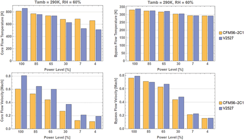
To consider another engine, in particular the V2527 engine used in ND-MAX/ECLIF2, the NPSS engine cycle code (Jones, 2007) was obtained from NASA and set up to first recalculate the CFM56 exhaust parameters. With very close agreement between the exhaust parameters for the CFM56 using both GasTurb and NPSS, the V2527 exhaust parameters were then calculated using NPSS and the computation matrix was recalculated for the V2527 engine, again at both 250 m and 1000 m downstream of the engine exit plane. This results in 45 + 5 [HC=0] cases for each of the two engines with output at two downstream distances (200 total output conditions including both engines). The exhaust parameters for the two engines are compared in Figure 1, where the differences between the temperature and velocity are evident, especially in the core flow, even though the trends and range of values are comparable between these engines.

Note that the comparison between these two engine thermodynamic cycles should not be construed as a comparison between the vPM emissions performance of these two engines. The emissions of the HCs in particular, but also the FSC are kept the same for these parametric studies and do not reflect the actual emissions performance of the actual engines. So, the comparison of these cases is to simply evaluate the impact of changing the engine exhaust parameters for representative cases. The differences are not large, so the other matrix parameters (HC level, HC profile, and FSC) are more important for determining the vPM evolution.

Figure 1. The flow temperatures and velocities calculated with NPSS are compared for the CFM56 and the V2527 across a range of power conditions (100, 85, 65, 30, 7, and 4% rated thrust). While the trends are similar for both engines, the distinct values are different, especially for the core, due to the differing designs of these two engines.

Time Evolution

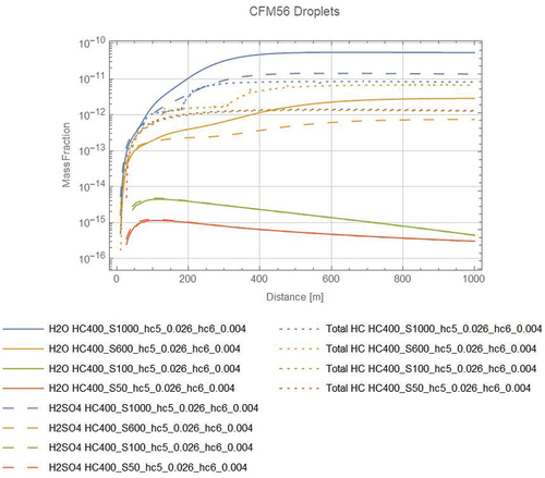
The ADSC model follows many parameters as the microphysical evolution is tracked downstream. It is not possible to simply display all of the parameters at once. To provide some perspective on the evolution of the microphysical environment, a time history of the mass fraction of the key contributions are shown in Figure 2. The H₂SO₄/H₂O contributions play a major role in the initial formation and growth of the droplets. The HC contribution for HC 400 ppbv is shown in this figure and represents a significant fraction of the mass for all the droplet cases plotted. The dependence on HC levels and profiles are discussed in more detail below and are documented in the SI.

Figure 2. The time histories, plotted versus downstream distance, of the condensed species in the droplet mode is tracked versus downstream distance. The total HC concentration is 400 ppbv and the Nom/Nom profile cases are shown for 4 sulfur levels. The 5 ppmm FSC level did not form droplets, so no curves are present in the figure for this case.

One of the more complex aspects of the vPM emissions is the creation of new particles and their subsequent growth. This is shown in Figures 3a and 3b. The bottom panel (3b) shows the creation of embryos, which are tracked by the number of sulfuric acid moieties in the cluster. Under conditions favorable to growth, the embryos become nm-sized droplets and often continue to grow significantly after that, as shown in the top panel (3a). The growth is usually dominated by HCs condensing on the embryos, unless there are very low or no HCs to condense or if there are very high H₂SO₄ levels. The variation on how the droplets depend on the HC conditions is explored in the subsequent matrix results.

Figure 3. The lower panel (3b) shows the formation and growth of embryos, which form the nuclei which also grow to become the droplets shown in the upper panel (3a). These are for the case 400 ppbv HC with a Nom/Nom profile and 100 ppmm FSC for the V2527 engine.

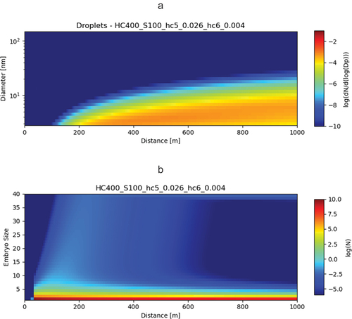
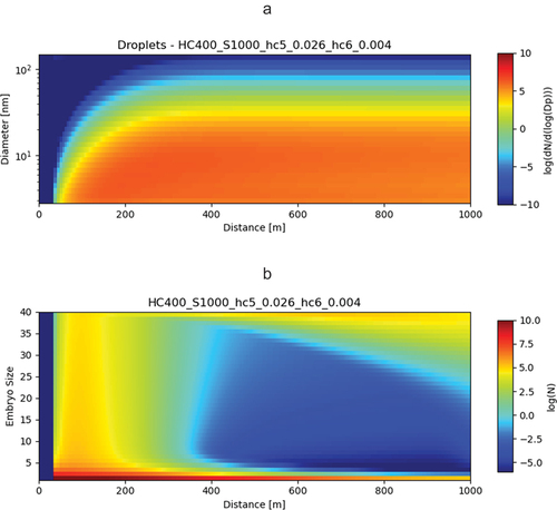
Figure 4. As Figure 3, the lower panel (4b) shows the formation and growth of embryos, which form the nuclei which also grow to become the droplets shown in the upper panel (4a). These are for the case 400 ppbv HC with a Nom/Nom profile and 1000 ppmm FSC for the V2527 engine.

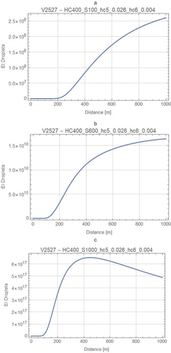
The EI_num based on the total number of droplets (upper panel Figure 3a, 4a and corresponding droplets for the 600 ppmm FSC case) is plotted in Figure 5. The initial rise is due to the formation and growth of the initial embryos, for all the figures 5a-c. For Figure 5c, the decay after about 400 m is due to the coagulation and the resulting evolution of the particle size distribution. The dilution due to the plume mixing is factored out by the EI calculation. The growth and possible decay depend on the concentrations of both H₂SO₄/H₂O and HC concentrations and the resulting particle numbers and available surface area for condensation.

Figure 5. The EI_num for the droplet mode is plotted versus downstream distance for the V2527 engine for the HC 400 ppbv, Nom/Nom profile case with a range of FSCs: Panel a) 100, Panel b) 600, and Panel c) 1000 ppmm

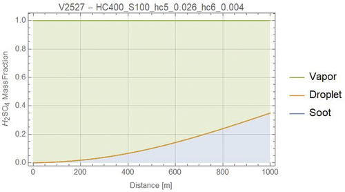
The partitioning between the gaseous phase (which is where all the condensable vPM precursors are at the beginning of the calculation,) the droplets, and coatings on the soot particles is shown for H₂SO₄ in Figure 6. It is notable that the droplets typically do not account for a large fraction of the H₂SO₄ mass fraction, even though their formation depends on the nucleation of embryos that are H₂SO₄/H₂O clusters. Also, as will be seen in the results later, it is somewhat counter intuitive that these droplets are usually dominated by HC contributions even though they begin as a H₂SO₄/H₂O cluster.

Figure 6. The partitioning of H₂SO₄ between the gas, droplet, and soot coating phases is shown versus downstream distance for the 400 pmmv, Nom/Nom, and FSC = 100 ppmm case for the V2527 engine.

It is also worth mentioning at this point that the ADSC code makes no provision for nucleation of new particles due to HCs only. No individual HC species becomes individually supersaturated in the diluting plume, so unary HC nucleation is not possible. Whether a higher order nucleation involving multiple HC species could occur was explored and found to be unlikely for baseline conditions when fuel S levels result in sulfuric acid in the exhaust. It is not clear that sufficient understanding of such a higher order HC nucleation exists to do such an analysis properly. For all the cases considered here, the nucleation of H₂SO₄/H₂O embryos is expected to occur before any HC nucleation would be expected, so HC nucleation and ion-induced nucleation for very low FSC levels is an open question for future studies.

Computational Matrix Output Pages

The computational matrix is a 45 element array of 3 total HC concentrations (133, 400, 1333 ppbv) times 5 sulfur levels (5, 50, 100, 600, 1000 ppmm) times three HC profiles (Nom/Nom, Nom/Low, Low/Low). An addition 5 calculations were done for the five FSCs with HC set to zero. This computation matrix was replicated for each of two engines (CFM56 and V2527) and output was generated at both 250 m and 1000 m downstream. Each of 4 HC (0, 133, 400, 1333 ppbv) concentrations is displayed in a figure in the Supplemental Information (SI) for each engine and both downstream distances, giving 16 (4 x 2 x 2) output figures. Each of the 16 figures in the SI has the 5 sulfur levels in rows stacked vertically, and the 3 HC profiles in columns spread horizontally (except for the 0 HC case, which has only one column filled). Each case is represented by a pie chart that has a diameter that scales with the total condensed mass of volatile material, and the wedges of the chart correspond to green for HCs, red for S, and blue for H₂O. In addition, quantitative values are displayed for labeling the pie charts’ compositional components. Above each pie chart, the estimated diameter (geometric mean diameter) of the resulting droplet is notated.

No droplet pie charts are shown for the FSC 5 ppmm cases (top row). These cases were run and typically embryos formed. However, the embryos did not grow to become droplets. Thus, no values can be given for droplets for these cases. It is significant that embryos are still present and this may be relevant for downstream emissions impacts. Another issue, though, is that the FSC 5 ppmm cases tended to have great difficulty in converging. The calculations are very unstable because the code is tracking in detail many species that are changing very little and the desired droplet parameters to be output are indeterminant as droplets never form. Usually, we were able to get the code to converge, and when the calculations did converge, they tended to provide values much like the HC=0 case with the same FSC value.

Also listed above each pie chart are two ratios. The first ratio, S/D, represents the ratio of total condensed mass in the corresponding soot coating compared to the total condensed mass in the droplets. This ratio does not include the underlying mass of the nvPM soot core, but rather tracks the amount of condensed mass in the soot coating mode versus that which is the droplet mode. While a similar, separate page could have been generated for the soot vPM contributions, the size of the soot is not usually affected much by the soot coatings, so nvPM diameter would not add much additional information. Thus, we decided to just present the soot coating total mass by providing the ratio to that in the droplets. Typically, the total vPM mass in the soot coatings is much greater than that in the droplets (S/D > 1), and the droplet total vPM mass only approaches or exceeds the soot coatings when there is an abundance of material to condense. Thus, the droplets only approach or exceed the coatings when the droplets have grown to significant sizes, which occurs only at either the highest HC values or the highest S values.

The other property of the soot coatings that is of interest is the composition of the soot coatings versus that of the droplets. All else being equal, one might expect the compositions to be the same. But sulfuric acid and HCs condense at different regimes in the plume, and the competition between droplets and soot particles can be different for HC and sulfuric acid vapors due to their different sizes and surface areas. So, an additional ratio was defined, R, which is the HC to S mass ratio of the soot coatings divided by the HC to S mass ratio of the droplets. If the vPM composition of both the droplets and the coatings are the same, R = 1. If R < 1, this means that the soot has a composition that is more weighted to sulfuric acid than does the droplets. In all cases, the soot has much more sulfuric acid rich composition than the droplets, although R approaches (from below) a few percent for very high S levels, where the droplets have grown significantly and consequently take up relatively more S, even if not as much as the soot coatings even at this highest R value.

Droplet Numbers

The droplet number emission indices, EIs, (effective, since these particles are not present at the engine exit plane) are tabulated in the SI for each of the 200 cases (Table A.1 at 250m and Table A.2 at 1000m). Number EIs are expressed as the number of particles per kg fuel burned, and so are independent of the subsequent dilution in the plume (scaling with CO₂, which dilutes in parallel). The detailed behavior shown in above Figure 5 is also evident in the Tables, with higher FSC resulting in more droplets. The FSC has the biggest impact on droplet numbers, with the HC level and profile having only a modest mediating impact on the numbers, even when the composition of the particles is dominated by HCs

Computational Matrix Results and Discussion

The results of the computational matrix are shown in the SI, with separate pages (16) for each engine (2), each downstream distance (2), and for each HC level (4). Several general comments can be made. Generally, the R values are much less than 1, indicating that most of the H₂SO₄ ends up on the soot. This is important, since it suggests that soot will always have H₂SO₄ on its surface when there is appreciable S in the fuel, even for low FSCs to 5 ppmm. This observation has significance for soot activation for contrails, since H₂SO₄ is highly hygroscopic and drives water condensation and contrail particle activation when it is present. These results strongly suggest that soot particles will be easily activated even for low FSCs for the range of aviation fuels expected in the foreseeable future. R approaches as much as a few percent at the highest FSC, which indicates that the droplet mode can approach that fraction of the H₂SO₄ for high FSCs, but the soot mode will also have abundant H₂SO₄ in such cases.

The droplets are often dominated by the HC (green) material. As mentioned above, this may be a little counter intuitive, since the ADSC code as run for these cases only allows the formation of H₂SO₄/H₂O embryos. Thus, the droplets start as H₂SO₄/H₂O embryos yet take up HCs more than do the coatings, which are initially a carbonaceous, hydrophobic surface. This is due to the dynamics of competition between the small droplets and the larger soot particles for the condensable species. At high FSCs combined with low HC levels, sulfuric acid can dominate the droplet composition.

Examining this in more detail, the composition of the droplets is compared to that of the soot coatings with the R ratio. In all cases, R <1. This means that the soot surface is more H₂SO₄-rich than are the droplets. R approaches a few percent from below only at the highest FSC, as described above. Thus, the composition of the droplets is more HC rich than the soot coatings. This trend has been observed experimentally in high FSC experiments, where the droplet mode becomes large enough to allow a compositional analysis to be performed (Peck et al., 2015; Yu et al., 2019).

The vPM properties are affected by the HC profile. Droplet size is largely determined by sulfate nuclei size and thus the FSC value. But increasing the total HC does add additional condensed mass. Changing the HC profile by decreasing the two heaviest HCs results in less HC material in the droplets, increasing the H₂SO₄ mass fraction. Decreasing both of the two heaviest HCs decreases the HC component more than just decreasing the single heaviest.

The amount of condensed mass in the soot coatings is often larger than that in the droplet mode (S/D > 1). For all but the largest droplet cases, which occurs when HCs are also the highest, the soot coatings have much more total condensed material. But when there is the most condensable material (highest FSC or high HC) available, the droplet mode can have similar total mass as the soot coatings, or even exceed the soot mode by a modest amount (S/D ≤ 1).

Generally, the droplet and coating properties evolve in regular and systematic ways as the various parameters are adjusted. One notable exception is the estimated particle diameter (DIA). As H₂SO₄ condenses, one would expect that particle size to grow, and this is usually seen such that DIA increases as FSC increases (embryos only at 5 ppmm, droplets less than a few nm in size for 50 ppmm, then several nm for 100 and 600). At 1000 ppmm FSC, the particle size decreases relative to 600 ppmm even though the total condensed mass is greater. These seemed anomalous, but upon further review, this case is explained by the fact that, for this very high FSC, the nucleation of embryos is so enhanced that the number of particles is significantly greater and the greater total mass in explained by an increase in the number of particles.

This result is interesting, since the particle number increase occurs at FSCs at and above the 600 ppmm FSC case. In a flight experiment (Schumann et al., 2002), similar behavior was observed at FSCs comparing 170 ppmm and 5500 ppmm. For FSCs below 1000 ppmm, the impact of varying FSC was not dramatic, yet for the 5500 ppmm case, the optical properties of the contrail changed. If the droplets in this flight experiment had become significantly numerous and with sizes approaching the size of the soot particles (see above discussion), then the droplets may start to become important as contrail particle nuclei that allow additional contrail particles to form and affect the contrail optical properties.

The two engines simulated in these calculations provide qualitatively similar results. The slightly cooler exhaust temperature for the V2527 at 7% rated thrust is probably the key difference that results in slightly higher HC contributions for these cases, due to a greater propensity to condense species sooner with the slightly cooler initial temperature. But each engine’s microphysical trends are similar with respect to the FSC, HC, and HC profile parameters.

Summary of Matrix Computations

An initial analysis of vPM has been performed to understand how FSC, HC concentration, and HC composition profiles affect the resulting vPM properties. While the calculations are computationally intensive and can experience numerical instabilities due to the stiffness of the differential equation system, the results show that both expected and unexpected trends occur.

For the two engines cycles that were evaluated, the changes in the vPM emissions are modest for these two engines of similar overall performance (similar thrust, size, and overall pressure ratio). The emissions parameters of HC level, HC profile, and FSC are more important in determining the vPM emissions characteristics. Note that for the engine cycles considered, the emissions levels studied were the same matrix for both engines. The actual emissions performance of these two engines are not identical, so the vPM results presented here do not provide an evaluation of the vPM emissions for these engines themselves. For engine cycles that are radically different from these cases, additional analysis would be needed to understand the impact on vPM

Generally, the condensed mass in the droplets and as coatings on soot particles increase as the condensable material increases, both FSC and HCs. The particle sizes tend to be primarily determined by FSC and increase with increasing FSC. However, the highest 1000 ppmm FSC shows a modest decrease in particle size relative to 600 ppmm, but with a significant increase in particle number. The effect of decreasing the amount of the heaviest, or most condensable, HC species is that the condensed HC material is decreased. This has significance if alternative jet fuels that have less aromatic content or a simpler HC matrix come into more extensive usage. Such changes in the fuel properties could result in changes in vPM emissions.

The newly formed droplets form as H₂SO₄/H₂O embryos yet grow to become HC-rich droplets except when H₂SO₄ levels are significantly more than that of HCs. Notably, the droplets that start off as H₂SO₄/H₂O embryos tend to be more HC rich than the coatings on the soot particles, which tend to have more a more H₂SO₄- and H₂O-rich composition than the droplets. The propensity for the soot to take up the H₂SO₄ has significance for contrail particle formation, since H₂SO₄ is highly hygroscopic. This suggests that H₂SO₄ can activate soot particles to be contrail particles even at quite low FSCs.

Parameterization of Results for Use in Models

The analysis presented above has made computations to 1 km (1000 m), which represents about 13 minutes of evolution from the engine exit plane for this low power engine condition. The calculations assume a quiescent ambient background (constant temperature and no wind). While this assumption may not be limiting in the near field plume of an aircraft engine, when extending to 13 minutes the ambient conditions begin to become much more important. While the ADSC results for the longer times are interesting and provide insight into subsequent evolution, they may not be representative for actual conditions of interest. In addition, as shown in the first-year results, the major activity in the microphysical evolution is most pronounced in the first 200 – 300 m of the plume. Activity after that point is more modest and is also more likely to be affected by ambient conditions.

For these reasons, and also informed by the temperature dependence study described below, it is suggested that the most useful ADSC results for low power engine conditions are the output at 250 m (49.2 s). The parameterization described below was thus done at both 250 m (49.2 s) and 1000 m (13.05 min), so that they are both available, but with the expectation that the nearer location would be most useful for application in local air quality models. Thus, the emphasis below is on this nearer location (250 m/49.2 s) which is of primary interest to the local air quality modeling community.

Parameterization of Computational Matrix Results

The computational matrix results provided the droplet and soot coating composition for a 45 element computation matrix made up of 5 sulfur levels (5, 50, 100, 600, 1000 ppmm) times 3 total HC concentrations (133, 400, 1333 ppbv) times three HC profiles (Nom/Nom, Nom/Low, Low/Low). For diagnostic purposes, the model was also run with sulfur included but the HCs set to zero (so no HC profile variation was needed). These additional 5 cases simply followed the microphysics of the sulfuric acid and water forming nuclei and interacting with the emitted nvPM, without including HC microphysics. This resulted in 45 + 5 [HC=0] cases for the each of the two engine cycles (CFM56 and V2527) that were considered, with output at two downstream distances (200 total output conditions including both engines). The difference in the composition between the two engine cycles, where the FSC and HC emissions were kept constant, were modest.

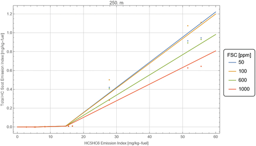
The results from the V2527 engine cycle are now been parameterized for use in simpler models, so that the complex ADSC code does not need to be run for each case within the range of parameters considered by the first-year computational matrix. It is noted that the dependence on HC was not dependent on the HC level and HC profile independently, but rather only depended on the sum of the two heaviest (lowest vapor pressure) HCs: HC⁵ (perylene: C₂₀H₁₂) and HC⁶ (Anthracene: C₂₂H₁₂). Thus, the parameterization was made in terms of the fuel sulfur content, FSC, and the concentration of the mass-weighted sum of HC⁵ and HC⁶, HC (0 < FSC < 1000 ppmm, 0 < HC < 20 ppbv). The equations for these parameterizations are included below and the parameterizations are plotted in Figures 7–16.

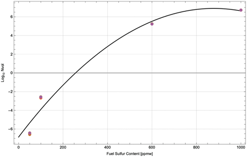
The HC content of the droplets and soot coatings are a function of both FSC and HC, and are linear in both those quantities, with a bilinear cross term. Thus, the HC parameterization is plotted as a two-dimensional contour plot as a function of FSC and HC (Figures 9, 10, 14, and 15). The SO₄ content of droplets and soot do not depend significantly on the HC inputs, but primarily on the FSC only. This is due to the low vapor pressure of H₂SO₄ causing more rapid condensation that precedes significant HC condensation. Thus, the SO₄ microphysics is not strongly affected by changes in the HC emissions. This also results in the droplet number density being primarily dependent only on the FSC. Thus, the SO₄ composition of droplets and soot coatings (Figures 7, 8, 12, 13) and the droplet number density (Figures 11 and 16) are plotted simply against the FSC.

Both the 250 m (Figures 7–12) and the 1000 m (Figures 13–16) results are shown. As discussed in the Introduction, the differences between the compositional parameterizations change in modest ways between 250 m and 1000 m. Thus, it is anticipated that the 250 m results will be most useful for local air quality modeling, where the evolution beyond 250 m can be tracked with the less detailed microphysics contained in downstream air quality models, which can also better include ambient conditions like temperature and local background emissions levels.

Figure 7. SO₄ content of droplets as a function of FSC at 250 m

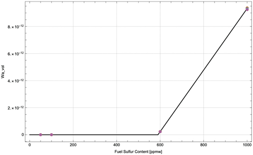
Figure 8. SO₄ content of soot coatings as a function of FSC at 250 m

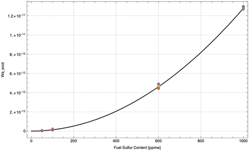
Figure 9. HC content of droplets as a function of HC and FSC at 250 m

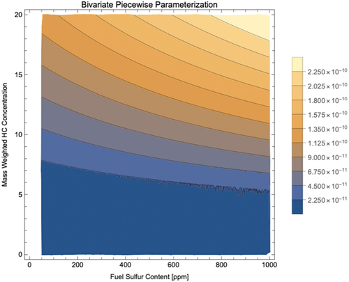
Figure 10. HC content of soot coatings as a function of HC and FSC at 250 m

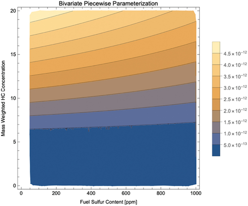
Figure 11. Number Density of droplets as a function of FSC at 250 m

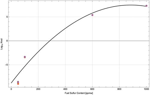
Figure 12. SO₄ content of droplets as a function of FSC at 1000 m

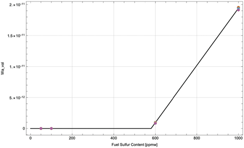
Figure 13. SO₄ content of soot coatings as a function of FSC at 1000 m

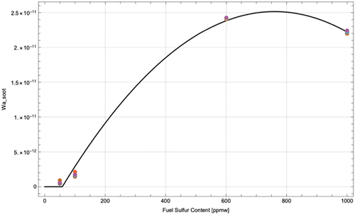
Figure 14. HC content of droplets as a function of HC and FSC at 1000 m

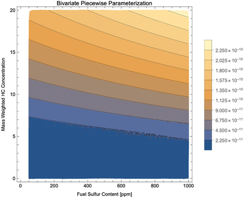
Figure 15. HC content of soot coatings as a function of HC and FSC at 1000 m

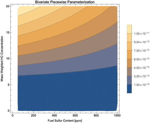
Figure 16. Number Density of droplets as a function of FSC at 1000 m

Temperature Dependence

The thermodynamics and microphysical evolution of the droplets and soot coatings are expected to be temperature dependent. Both engine exit temperature and the ambient temperature (which is an important parameter for determining the engine exit temperature as well) are important inputs to the ADSC calculation. The computational matrix was run for a nominal ambient temperature and it was decided to consider additional calculations at a colder temperature to explore the changes in composition due to reduced temperature. Increased condensation is expected at colder temperatures and, if the changes in composition could be simply parameterized, it would extend the usefulness of this modeling effort if the temperature dependence could also be included.

In order to examine the temperature dependence, additional calculations with the ADSC code were done at 273 K (0ºC). To prepare for these calculations, the engine cycles also had to be recalculated using NPSS for the altered ambient conditions. Rather than calculate the full complete computational matrix, a diagonal set of conditions were chosen: a low S, low HC case: a middle S, middle HC case; and a high S, high HC case (HC133/S50; HC400/S100; HC1333/S1000). This would span a range of cases and would provide insight into the nature of the temperature dependences of both SO₄ and HCs. Additional ADSC calculations were done for these “diagonal” conditions at the lower temperature.

In analyzing the output of these new, lower temperature cases, it was quickly determined that the best point of comparison was to compare the Emission Indices (EIs, g [species X]/kg fuel, again independent of dilution, like the number EI) of SO₄ and the sum of HC⁵ and HC⁶. The EIs account for any changes in fuel flow in the engine due to changes in the ambient temperature, as well as properly accounting for the dilution in the exhaust plume.

However, ADSC was not set up to calculate the EIs for the sum of HC⁵ and HC⁶, and the available output is not sufficiently complete to calculate the EIs from the available output. Thus, the ADSC code needed to be modified to explicitly output the quantities of interest. With the modified code, the lower temperature calculation could be rerun. However, since the initial results were run with the unmodified code, the “diagonal” conditions also needed to be rerun for the original, nominal ambient temperature in order to get the relevant EIs with which to compare. Due to the difficulties in getting convergence for these very stiff differential equations, multiple runs needed to be done with various tolerances to obtain all of the relevant output. While not as time consuming as the original computational matrix, significant effort was needed to complete the temperature dependence calculations.

The results shown in Table 2. The tabulated values are the ratios of the EIs at the colder temperature 273 K (0ºC) to that at the warmer temperature 290 K (17ºC). This shows how the composition increases as the temperatures drop for ratios great than 1. Indeed, except for the highest HC case for H₂SO₄ in the soot coatings, all of the values in Table 2 are close to 1 or greater than 1 (sometimes much greater). This indicates that there is generally more vPM mass as the temperature drops, as expected.

However, simple trends are not easily extracted. There is competition between the droplets and soot coatings for H₂SO₄ and HCs, and the two species also compete with each other in both modes. So the temperature trends can be different at 250 m (49.2 s) versus 1000 m (13.05 min) and for H₂SO₄ versus HCs. It is worth noting that H₂SO₄ in the soot coatings are less affected than the H₂SO₄ on droplets, and most of the H₂SO₄ is contained in the soot coatings. Further, the HCs in the soot coatings have large, indeterminate changes for cases where the HCs are very small (HC133/S50 cases for soot at both 250 and 1000 m). Thus, changes can be quite large when the compositional contribution is very minor. Presumably, this does not affect the total mass in a major way. Similarly, the H₂SO₄ in droplets is complicated and depends on HC level and T but has very large changes primarily when the HCs dominate. Thus, again, the effect on the total mass is not expected to be major.

All of this suggests that there is no simple parameterization of the temperature dependence for the total H₂SO₄:HC/droplet:coating system. Again, generally there is more total vPM mass as the temperature drops. The H₂SO₄ on soot coatings is less affected than H₂SO₄ on droplets and the HC contribution (HC⁵+HC⁶) in droplets is less affected when there are large HC contributions. But the behavior of the H₂SO₄ contributions in droplets is complicated and depends on HC level and temperature in complex ways. The H₂SO₄ can experience very large changes, but this often occurs when HCs dominate the total mass.

The conclusion to draw from this temperature study is that the temperature dependence of this H₂SO₄:HC/droplet:coating system is complex in detail. No simple parameterization of the full microphysics is possible. Either a very complex temperature dependence would need to be parameterized as a function of T and the HCs, H₂SO₄, soot, and droplets properties or, alternatively, a full ADSC calculation would need to be calculated for each condition explicitly. Both of these options are prohibitively computationally expensive. Perhaps a better solution is to allow the evolution of the vPM to be modeled by local air quality models using the 250 m (49.2 s) conditions as input. While this does not account for changes in the initial emissions from the engine and the microphysics that occurs in the first 49.2 s, the subsequent thermodynamic evolution in the local air quality modeling may compensate for some of the initial microphysics that is lost by this approach. This “earlier hand-off” is consistent with the arguments given above to provide the results of this modeling study for the 250 m (49.2 s) output location for use in subsequent modeling.

Table 2. Ratio of EI_{273 K}/EI_{290 K} for H₂SO₄ and HCs for droplets and soot coatings at both 250 m (49.2 s) and 1000 m (13.05 min) for the “diagonal” matrix cases.

250 m	Sulfuric Acid		Organics
	Droplets	Soot	Droplets	Soot
HC113/S50	18.5	0.892	71.7	∞
HC400/S100	49.1	1.01	8.68	59.2
HC1333/S1000	203	0.122	1.58	18.3
1000 m	Sulfuric Acid		Organics
	Droplets	Soot	Droplets	Soot
HC113/S50	∞	0.311	642	∞
HC400/S100	515	1	23.9	41.9
HC1333/S1000	74.2	0.0909	1.5	10.4

Polydisperse Soot Distribution Effects on Composition

In order to keep the ADSC computations somewhat tractable, all of the matrix calculations were done assuming that the soot size distributions were monodisperse. That is to say, the size distributions were given a nominal average size and all of the particles had the same size, with zero width to the size distribution. Thus, the particle size distribution had only one bin, and this kept the computational complexity tractable. Spreading the size distribution over additional bins would increase both the computer memory requirements and the computational complexity of the overall computation. However, a monodisperse size distribution is physically unrealistic and there were concerns whether that would affect the ADSC computed results on the composition and number density of the droplets and, especially, the composition of the soot coatings.

While redoing all of the computational matrix with a polydisperse size distribution would require too much computational expense, it was decided to attempt to do a single representative matrix element with a polydisperse soot size distribution to ascertain whether that case showed a significant difference between poly- and monodisperse results. While a highly resolved size distribution (many size bins) would quickly become computationally excessive, both 2 bin and 5 bin cases were started for a central matrix element. Some numerical issues were encountered, which required computational adjustments of the differential equation solver tolerances, and the cases were allowed to proceed. The results for the 5 bin distribution calculation suggest that there is little compositional variation across most of the size distribution, with modest differences between HC⁵ and HC⁶ levels in small end tail of the distribution (10s of % change in composition). But with less mass in the smaller particles, the average composition is not likely to be strongly affected. This indicates are that the monodisperse calculations provide a good approximation of the compositional results for both the droplets and soot coatings when compared to a more representative polydisperse soot size distribution calculation.

Summary of vPM Parameterization

The results from the computational matrix have been parameterized with simple expressions so that the vPM behavior can be represented in simpler microphysical models that are used in local air quality modeling tools. The approach and results are summarized here for use by the local air quality modeling community.

The temperature dependence of the HC and SO₄ composition of the droplets and soot coatings has been explored. It has been determined that the microphysical behavior is complex and interrelated between H₂SO₄ and the sum of HC⁵ and HC⁶, as well as between droplets and soot coatings. Thus, there is no simple parameterization of the temperature dependence. Rather than doing detailed ADSC microphysical calculations for each case, it is recommended to provide early (250 m/49.2 s) output from ADSC to subsequent modeling, to allow those downstream, simpler microphysical models to track the microphysical evolution of the vPM.

Using a polydisperse soot size distribution has shown that there are no significant differences relative to the approximation of using a monodisperse size distribution. The monodisperse approximation provides a good indication of the droplet properties and the soot coating composition.

Parameters to use in vPM modeling

A new parameterization is offered that could be used to give more detail for vPM modeling. Beyond the masses of condensed S and condensed HCs, the new parameterizations provides:

• Mass, composition, and number for droplets

• Mass and composition of coatings on the emitted nvPM (soot)

The parametric study provides five quantities of interest (with dependence on input parameters):

1. The sulfuric acid and water content of the droplets (linear in FSC x ε)

2. The organic content of the droplets (bilinear in HC and FSC x ε)

3. The number of droplets (log of EI_num is quadratic in FSC x ε)

4. The sulfuric acid and water content of the soot coatings (quadratic in FSC x ε)

5. The organic content of the soot coatings (bilinear in HC and FSC x ε)

The coefficients for each of these five quantities are shown below. Note that for the organic contents, there are three regions of bilinear behavior that are defined by the HC level, but the behavior in each region is bilinear.

The inputs for these equations are the FSC, ε, and the condensable HCs. The FSC is presumably known for the scenario of interest. The sulfur conversion (how much of the FSC is converted to S(VI), i.e. initially SO₃ and soon thereafter to H₂SO₄) is also a modeling input and is typically of the order of 1%. The amount of condensable organics in the gas phase is difficult to predict or measure. In FOA (3 and 4), the amount of condensed HC that was measured in APEX1 from a CFM56-2C1 engine was used, which is the output. The amount of vapor phase condensable organics was not available. If the condensed phase HCs are used as the input, this assumes that all of the condensable organics condense from the vapor phase to the particle phase, which is not the case in the modeling results from the present study. However, in many cases a large fraction of the condensable HCs do condense by the 50 s (250 m) downwind station.

Thus, the same inputs as used in FOA4 can be used for the parametric equations presented here (FSC, ε, and the condensable HCs).

The parametric equations for each quantity of interest are presented below:

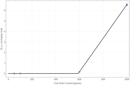
1) The sulfuric acid and water content of the droplets (linear in FSC x ε)

${\text{EI}}_{\text{SO4\_droplets}}\text{(mg/kg}-\text{fuel)}=\{\begin{array}{cc}\mathrm{0,}& \text{FSC}\mathit{ϵ}\le 5.898\\ -9.417+1.597\text{FSC}\mathit{ϵ}\mathrm{,}& \text{True}\end{array}$

Figure 17. The sulfuric acid and water content of the droplets

2) The organic content of the droplets (bilinear in HC and FSC x ε)

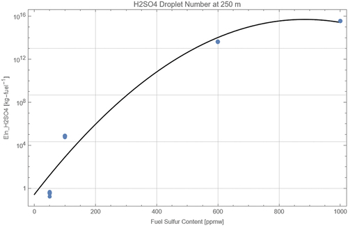
3) The number of droplets (log of EI_num is quadratic in FSC x ε)

${\text{EI}}_{\text{HC\_droplets}}\text{(mg/kg}-\text{fuel)}=\{\begin{array}{cc}6.907\times {10}^{-4}\text{EIHCFSC}\mathit{ϵ}+0.001349\text{EIHC}\mathrm{,}& \text{1.EIHC}<5.322\\ 0.04854\text{EIHCFSC}\mathit{ϵ}-0.01142\text{EIHC}-0.2547\text{FSC}\mathit{ϵ}+\mathrm{0.06797,}& 0.3476\text{EIHC}-\frac{5.566}{\text{FSC}\mathit{ϵ}+36.90}<5.128\\ 0.06669\text{EIHCFSC}\mathit{ϵ}+0.6580\text{EIHC}-0.5224\text{FSC}\mathit{ϵ}-\mathrm{10.10,}& \text{True}\end{array}$

Figure 18. The organic content of the droplets

${\text{EI}}_{\text{num}}\text{(\#/kg}-\text{fuel)}=1.686\times {10}^8\times {10}^{-8.794+3.681\text{FSC}\mathit{ϵ}-0.2082{\text{FSC}}^2{ϵ}^2}$

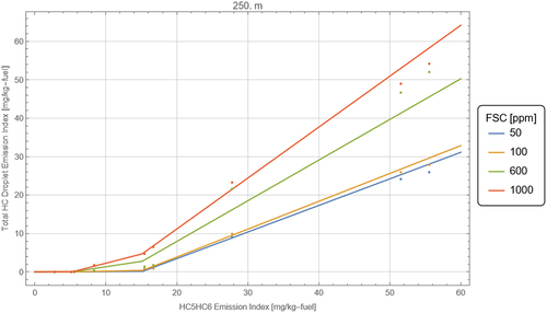
Figure 19. The number of droplets

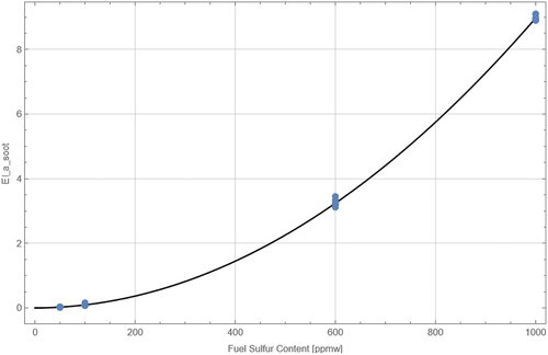
4) The sulfuric acid and water content of the soot coatings (quadratic in FSC x ε)

${\text{EI}}_{\text{SO4\_soot}}\text{(mg/kg}-\text{fuel)}=-5.787\times {10}^{-4}+0.005102\text{FSC}\mathit{ϵ}+0.08915{\text{FSC}}^2{ϵ}^2$

Figure 20. The sulfuric acid and water content of the soot coatings

5) The organic content of the soot coatings (bilinear in HC and FSC x ε)

${\text{EI}}_{\text{HC\_soot}}\text{(mg/kg}-\text{fuel)}=\{\begin{array}{cc}5.374\times {10}^{-7}\text{EIHCFSC}\mathit{ϵ}+2.247\times {10}^{-5}\text{EIHC}\mathrm{,}& \text{1.EIHC}<5.322\\ -9.840\times {10}^{-6}\text{EIHCFSC}\mathit{ϵ}+9.748\times {10}^{-4}\text{EIHC}+5.523\times {10}^{-5}\text{FSC}\mathit{ϵ}-\mathrm{0.005069,}& 0.3476\text{EIHC}-\frac{2.883}{27.84-\text{FSC}\mathit{ϵ}}<4.969\\ -9.508\times {10}^{-4}\text{EIHCFSC}\mathit{ϵ}+0.02718\text{EIHC}+0.01351\text{FSC}\mathit{ϵ}-\mathrm{0.3874,}& \text{True}\end{array}$

Figure 21. The organic content of the soot coatings

Acknowledgments

Funding support by the US FAA via JD RoVolus Contract Number 693KA9-18-D-00005 (TO26) is gratefully acknowledged. Useful technical discussions during the course of the work with Dr. S. Daniel Jacob of the FAA Office of Environment and Energy are also much appreciated.

Data Availability Statement

The authors confirm that the data supporting the findings of this study are available within the article and its supplementary materials.

Additional information

Funding

The work was supported by the Federal Aviation Administration [JD RoVolus Contract Number 693KA9-18-D-00005 (TO26].

References

- Anderson, B.E., A.J. Beyersdorf, C.H. Hudgins, J.V. Plant, K.L. Thornhill, E.L. Winstead, L.D. Ziemba, R. Howard, E. Corporan, R.C. Miake-Lye, S.C. Herndon, M. Timko, E. Woods, W. Dodds, B. Lee, G. Santoni, P. Whitefield, D. Hagen, P. Lobo, W.B. Knighton, D. Bulzan, K. Tacina, C. Wey, R. VanderWal, and A. Bhargava, (2011), Alternative Aviation Fuel EXperiment (AAFEX). Report No. NASA/TM-2011-217059.
- Corbin, J.C., T. Schripp, B.E. Anderson, G.J. Smallwood, P. LeClercq, E.C. Crosbie, S. Achterberg, P, D. Whitefield, R.C. Miake-Lye, Z. Yu, A. Freedman, M. Trueblood, D. Satterfield, W. Liu, P. Oßwald, C. Robinson, M.A. Shook, R.H. Moore, and Prem Lobo, (2022), Aircraft-engine particulate matter emissions from conventional and sustainable aviation fuel combustion: comparison of measurement techniques for mass, number, and size, Atmos. Meas. Tech.. 15, 3223–3242, https://doi.org/10.5194/amt-15-3223-2022.
- Davidson, M.J., and H.J. Wang. 2002. Strongly Advected Jet in a Coflow. J. Hydraul. Eng. 128 (8):742–52. doi:10.1061/(ASCE)0733-9429(2002)128:8(742).
- Fushimi, A., K., Saitoh, Y. Fujitani, and N. Takegawa, (2019), Identification of jet lubrication oil as a major component of aircraft exhaust nanoparticles, Atmos. Chem. Phys.. 19, 6389–6399, https://doi.org/10.5194/acp-19-6389-2019.
- Hudda, N. and S.A. Fruin, (2016), International Airport Impacts to Air Quality: Size and Related Properties of Large Increases in Ultrafine Particle Number Concentrations, Environ. Sci. Technol.. 50, 3362–3370, https://doi.org/10.1021/acs.est.5b05313.
- ICAO, Airport Air Quality Manual, (2011), https://www.icao.int/publications/Documents/9889_cons_en.pdf
- ICAO, Volume II, Annex 16, (2019), https://store.icao.int/en/annex-16-environmental-protection-volume-ii-aircraft-engine-emissions.
- ICAO, Emissions databank. (2020), https://www.easa.europa.eu/domains/environment/icao-aircraft-engine-emissions-databank.
- Jones, S.M., (2007), An introduction to thermodynamic performance analysis of aircraft gas turbine engine cycles using the Numerical Propulsion System Simulation code, NASA/TM—2007-214690.
- Kılıç, D., I. El Haddad, B.T. Brem, E. Bruns, C. Bozetti, J. Corbin, L. Durdina, R.-J. Huang, J. Jiang, F. Klein, A. Lavi, S.M. Pieber, T. Rindlisbacher, Y. Rudich, J.G. Slowik, J. Wang, U. Baltensperger, and A.S/H. Prévôt, (2018), Identification of secondary aerosol precursors emitted by an aircraft turbofan, Atmos. Chem. Phys. 18, 7379–7391, https://doi.org/10.5194/acp-18-7379-2018
- Kurzke, J., 2004, GasTurb 10: A Program for Gas-Turbine Performance Calculations, Dr. Joachim Kurzke, Dachau, Germany.
- Moore, R.H., M. Shook, A. Beyersdorf, C. Corr, S. Herndon, W.B. Knighton, R. Miake-Lye, K.L. Thornhill, E.L. Winstead, Z. Yu, L.D. Ziemba, and B.E. Anderson, (2015), Influence of Jet Fuel Composition on Aircraft Engine Emissions: A Synthesis of Aerosol Emissions Data from the NASA APEX, AAFEX, and ACCESS Missions, Energy Fuels, 29, 2591–2600, 10.1021/ef502618w.
- Peck, J., Z. Yu, R.C. Miake-Lye and D.S. Liscinsky, (2015), A Volatile Particle Microphysical Simulation Model for the Evolution of Surrogate Organic Emissions in an Aircraft Exhaust Plume, TAC-4 Proceedings, June 22nd to 25th, 2015, Bad Kohlgrub, p. 21.
- SAE, (2011), SAE ARP1179D, Aircraft Gas Turbine Engine Exhaust Smoke Measurement Pittsburgh PA.
- Schripp, T., B.E. Anderson, U. Bauder, B. Rauch, J.C. Corbin, G.J. Smallwood, P. Lobo, E.C. Crosbie, M.A. Shook, R.C. Miake-Lye, Z. Yu, A. Freedman, P.D. Whitefield, C.E. Robinson, S.L. Achterberg, M. Köhler, P. Oßwald, T. Grein, D. Sauer, C.Voigt, H. Schlager, and P. LeClercq, (2022), Aircraft engine particulate matter emissions from sustainable aviation fuels: Results from ground-based measurements during the NASA/DLR campaign ECLIF2/ND-MAX, Fuel, 325, 124764, https://doi.org/10.1016/j.fuel.2022.124764.
- Schumann, U., F. Arnold, R. Busen, J. Curtius. B. Kärcher, A. Kiendler, A. Petzold, H.Schlage, F. Schröder, and K.-H. Wohlfrom, (2002), Influence of fuel sulfur on the composition of aircraft exhaust plumes: The experiments SULFUR 1-7, J. Geophys. Res. 107, D15, 10.1029/2001JD000813, 2002.
- Timko M.T., S.C. Herndon, E.C. Wood, T.B. Onasch, M.J. Northway, J.T. Jayne, M.R. Canagaratna, R.C. Miake-Lye, and W. Berk Knighton. 2010a. Gas Turbine Engine Emissions—Part I: Volatile Organic Compounds and Nitrogen Oxides. J. Eng. Gas Turbines and Power 132 (6):061504–1. doi:10.1115/1.4000131.
- Timko M.T., T.B. Onasch, M.J. Northway, J.T. Jayne, M.R. Canagaratna, S.C. Herndon, E.C. Wood, R.C. Miake-Lye, and W. Berk Knighton. 2010b. Gas Turbine Engine Emissions— Part II: Chemical Properties of Particulate Matter. J. Eng. Gas Turbines and Power 132 (6):061505–1. doi:10.1115/1.4000132.
- Ungeheuer, F., D. van Pinxteren, and A.L. Vogel, (2021), Identification and source attribution of organic compounds in ultrafine particles near Frankfurt International Airport Atmos. Chem. Phys.. 21, 3763–3775, https://doi.org/10.5194/acp-21-3763-2021.
- Wayson, R.L., G.G. Fleming, and R. Iovinelli, (2009), Methodology to Estimate Particulate Matter Emissions from Certified Commercial Aircraft Engines, J. Air & Waste Manage. Assoc. 59, 91–100.
- Wey, C. C., B. E. Anderson, C. Wey, R.C. Miake-Lye, P. Whitefield, and R. Howard, (2007), Overview on the Aircraft Particle Emissions Experiment, J. Propulsion and Power, 23, 898–905.
- Wong, H.-W., and R.C. Miake-Lye. 2010. Parametric studies of contrail ice particle formation in jet regime using microphysical parcel modeling. Atmos. Chem. Phys. 10 (7):3261–72. doi:10.5194/acp-10-3261-2010.
- Wong, H.-W., M. Jun, J. Peck, I.A. Waitz, and R.C. Miake-Lye. 2014. Detailed microphysical modeling of the formation of organic and sulfuric acid coatings on aircraft emitted soot particles in the near field. Aerosol Sci. Technol. 48 (9):981–95. doi:10.1080/02786826.2014.953243.
- Wong, H.-W., M. Jun, J. Peck, I.A. Waitz, and R.C. Miake-Lye. 2015. Roles of organic emissions in the formation of near field aircraft-emitted volatile particulate matter: a kinetic microphysical modeling study. J. Eng. Gas Turbines and Power 137 (7):072606–1. doi:10.1115/1.4029366.
- Yu, Z., M.T. Timko, S.C. Herndon, R.C. Miake-Lye, A.J. Beyersdorf, L.D. Ziemba, E.L. Winstead, and B.E. Anderson. 2019. Mode-specific, semi-volatile chemical composition of particulate matter emissions from a commercial gas turbine aircraft engine. Atmos. Environ. 218:116974. doi:10.1016/j.atmosenv.2019.116974.