Repeated sampling with a black box to make informal statistical inference accessible

ABSTRACT

While various studies suggest that informal statistical inference (ISI) can be developed by young students, more research is needed to translate this claim into a well-founded learning trajectory (LT). As a contribution, this paper presents the results of a cycle of design research that focuses on the design, implementation, and evaluation of the first part of an LT for ISI, in which ninth-grade students (N = 20) are introduced to the key concepts of sample, frequency distribution, and simulated sampling distribution. The results show that an LT starting from repeated sampling with a black box may support the accessibility of these concepts, as these students were able to make inferences with the frequency distribution from repeated samples as well as with corresponding simulated sampling distributions. This suggests a promising way to make ISI more accessible to students.

KEYWORDS:

• Design research
• informal statistical inference
• learning trajectory
• repeated sampling
• statistics education

Drawing inferences about an unknown population is at the heart of statistics, and therefore important to learn. Sample data are commonly used to reason about a larger whole. For informed citizenship in a society in which data play an increasingly important role, reasoning with statistical information is essential (Gal, 2002). As such, statistical reasoning is considered as one of the 21st-century skills that students should acquire (Thijs, Fisser, & Van der Hoeven, 2014).

However, learning and applying statistical inference is difficult for students. The emphasis on formal and procedural knowledge results in the inability of students to interpret the results (Castro Sotos, Vanhoof, Van den Noortgate, & Onghena, 2007) or to understand statistical concepts such as sampling, variation, and uncertainty (Konold & Pollatsek, 2002).

Recent research suggests that studying informal statistical inference (ISI) at an early age may facilitate the later transition to formal procedures (Zieffler, Garfield, delMas, & Reading, 2008). In general, ISI focuses on ways in which students without knowledge of formal statistical techniques, such as hypothesis testing, use their statistical knowledge to support their inferences about an unknown population based on observed samples. Although ISI has several definitions, the commonly used framework from Makar and Rubin (2009) identifies three key principles: generalization beyond data, data as evidence for these generalizations, and probabilistic reasoning about the generalization. At an informal level, familiar experiences can be used for making such inferences. By turning common predictions and expectations into inference processes, interpreting and understanding statistical concepts become more accessible (Paparistodemou & Meletiou-Mavrotheris, 2008).

Although various studies have shown that ISI can be developed in young students (Ben-Zvi, 2006; Doerr, delMas, & Makar, 2017; Makar, 2016; Meletiou-Mavrotheris & Paparistodemou, 2015) more research is needed to translate these promising results into compact theoretically underpinned learning trajectories in which students are introduced to sampling and the associated probability component in a short period of time. In particular, it is important to investigate how students can learn to draw informal inferences and what learning steps are needed to develop this ability among young students, as well as which learning activities may foster these learning steps. In most countries, school curricula for grades 7–9 focus on descriptive statistics (Ben-Zvi, Bakker, & Makar, 2015) and, as a result, pay little attention to informal statistical inference. This also holds for the Dutch curriculum, in which statistics education progresses from descriptive statistics in the early years, to prepare for a more formal approach to inferential statistics from grade 10 and in higher education (Van Streun & Van de Giessen, 2007). As time in educational practice is limited, both in the Netherlands and abroad, we aim for a concise approach.

This research focuses on the question of how to provide students with opportunities to learn to draw conclusions about a population based on samples. To provide an answer to such a how-question we look for an idea of how such a learning goal can be achieved (design), to implement this idea, and to find evidence that the learning goal was indeed achieved. Hence, the aim of the research reported here is to design, implement, and evaluate the first part of a learning trajectory (LT) for ninth-grade students, that focuses on informal inferential reasoning and three statistical key concepts of sample, frequency distribution, and simulated sampling distribution.

Theoretical background

To set up the study’s theoretical background, we now elaborate the role of informal inferential reasoning and the key statistical concepts to enhance ISI.

The role of inferential reasoning to enhance ISI

This research focuses on inferential reasoning underpinning interpretations of sample data. In contrast to descriptive statistics, which concerns describing the data under investigation, inferential reasoning includes handling sampling variation and uncertainty. An inferential statement is fairly meaningless without the reasoning in which it must be embedded (Makar, Bakker, & Ben-Zvi, 2011). Therefore, an inference should be accompanied by reasoning based on the data. Following Zieffler et al. (2008), we consider informal inferential reasoning as making inferences about unknown populations based on observed samples without using formal techniques such as hypothesis testing using probability distributions. Informal inferential reasoning is about drawing on, utilizing, and integrating knowledge from meaningful experiences, as decisions are commonly made on the basis of predictions and estimates. These experiences can be used to make statistical concepts accessible. Informal inferential reasoning may include foundational statistical concepts, such as the notion that a sample may be surprising given a particular claim and the use of statistical language.

Key statistical concepts for ISI

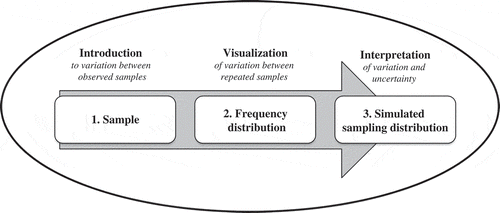
Informal inferential reasoning, and the use of statistical concepts to seek evidence for interpretations of data, can be developed through various experiences with data over time (Makar et al., 2011). The question is which statistical concepts are important for ninth-grade students who are inexperienced with sampling. From the literature, three concepts appear to be central: (1) sample (including ideas of sampling variation, sample size, and repeated samples), (2) frequency distribution of data obtained from repeated sampling, and (3) simulated sampling distribution. Figure 1 provides an overview of the three central aspects and the build-up in handling variation and uncertainty: from the introduction to variation in observed samples, by visualizing variation within a frequency distribution, towards interpreting variation and uncertainty of samples with the simulated sampling distribution, which we elaborate on below.

Figure 1. Overview of key concepts for ISI and the connection with handling variation and uncertainty.

First, inferential reasoning involves understanding the concept of sample. However, students are often reported to have conceptual problems with samples. On the one hand, students may assume every sample to be different and are therefore hesitant to draw conclusions about a population (Ben-Zvi, Aridor, Makar, & Bakker, 2012). On the other hand, students may consider a sample as a mini-population with the same characteristics as the underlying population and, as a consequence, students expect a small sample size to be a good reflection of the underlying population (Tversky & Kahneman, 1971). This is confirmed by Innabi and El Sheikh (2007), who showed that students in grade 11 did not take the sample size into account when interpreting sample results. Students often make grand statements based on small samples and are insufficiently aware of the role of sample size. Experimenting with repeated sampling enables students to become aware of the variation and uncertainty of a sample, but also of the “representativeness” of a sample (Saldanha & Thompson, 2002). Through repeated sampling, students are confronted with both variation and similarities, which allows them to gain insight into the variation versus stability of particular characteristics. Wild, Pfannkuch, Regan, and Horton (2011) invited students to experiment with various sample results from a given population, with variation in sample size and sample repetitions, to raise awareness and understanding of sampling variation. In this respect, Wild and Pfannkuch (1999) emphasized the importance of the exchange and comparison of sample results. Although repeated samples vary, some sample results are more likely than others. Thinking about the question: “What happens if a sample is repeated?” contributes to getting a grip on variation and uncertainty. This “what if” question is paramount in understanding statistical inference (Rossman, 2008).

With respect to the second key concept, a graph of the frequency distribution from repeated samples allows for visualization of obtained results and gives an overview of variation and stability among samples. A sample leads to data, a dataset has particular characteristics (such as proportion), and these characteristics are compiled in the frequency distribution of results from repeated sampling. The horizontal axis of a graph of such a distribution contains the values of the dataset characteristic. The vertical axis shows the number of samples for which each value occurred. A graph of the frequency distribution from repeated samples can be made manually or by using a computer and gives insight into (un)likely sample results. As such, the graph of the frequency distribution functions as a model of obtained results from repeated sampling and can be used to display sampling variation and, as a next step, to further investigate variation and uncertainty.

As a third key concept, the simulated sampling distribution can be utilized as a model for making statements about variation and uncertainty. If used as intended, the simulated sampling distribution extends the concept of frequency distribution from step 2, that functioned as a model (or visualization) of obtained sample results. Experts in statistics may think of these as conceptually the same (cf. Sfard & Lavie, 2005), but from a learning perspective, there may still be a developmental transition from a model of into a model for (Gravemeijer, 1999). The switch from a visualization of specific datasets to a more abstract simulation model for interpreting variation and uncertainty, we assume, enables emergent statistical reasoning. Such a sampling distribution, based on a large number of simulations, can easily be made with computer software (such as TinkerPlots). This simulated sampling distribution can be used to determine informally the probability of certain sample results (Rossman, 2008; Watson & Chance, 2012) and can assist in determining whether a sample result is likely (Garfield, Ben-Zvi, Le, & Zieffler, 2015; Manor & Ben-Zvi, 2015; Pfannkuch, Ben-Zvi, & Budgett, 2018; Watson & Chance, 2012). Reasoning with the sampling distribution from repeated sampling is a meaningful preparation for the more formal reasoning with the theoretical sampling distribution in higher education (Garfield et al., 2015; Watson & Chance, 2012).

The black box activity in the research of Van Dijke-Droogers, Drijvers, and Bakker (2018) seemed a promising way to introduce students to the key statistical concepts of ISI. Here, students investigated the content of a black box filled with marbles by gathering, exchanging, and comparing results from physical and later simulated samples with different sizes and different number of repetitions.

Research question

Given the importance of informal inferential reasoning and the corresponding key concepts in enhancing ISI, the main question of this research is: How can repeated sampling with a black box introduce ninth-grade students to the concepts of sample, frequency distribution, and simulated sampling distribution?

Methods

Over the past 10 years, research has increasingly focused on informal statistical inference and has developed various educational materials for young students (Doerr et al., 2017; Meletiou-Mavrotheris & Paparistodemou, 2015). However, educational resources and teaching materials in which ninth-grade students are introduced to the concepts of sample, frequency distribution, and simulated sampling distribution in a short period of time hardly exist. Therefore, this research required a design research approach. Design research is characterized by a cyclical process in which educational materials for learning environments are designed, implemented, and evaluated, for following cycle(s) of (re)design and testing (McKenney & Reeves, 2012). The research reported here comprised a first cycle of design, implementation, and evaluation of an LT for ISI. We focused on the first steps, as part of a longer LT. We designed a hypothetical learning trajectory (HLT) of eight steps to map out and structure all elements involved in the learning and teaching approach, and to make explicit the expectations about how these elements function in interaction to promote learning. The LT was implemented and tested during a classroom intervention. Here, we report on the design, implementation, and evaluation of the first three steps and indicate how the results of these steps were used for revision.

HLT as a design research instrument

As a design and research instrument to structure and connect the elements involved in an LT, we used a hypothetical learning trajectory (HLT). According to Simon (1995), who introduced this notion, and Simon and Tzur (2004), an HLT consists of a learning goal for students, a description of promoting activities that will be used to achieve these goals, and hypotheses about the students’ learning process. It includes the simultaneous consideration of mathematical goals, student thinking models, teacher and researcher models of students’ thinking, sequences of teaching tasks, and their interaction at a detailed level of analysis of processes (Clements & Sarama, 2004). Research by Gravemeijer, Bowers, and Stephan (2003) showed how an HLT can be used to bridge the gap between students’ ideas and solutions on the one hand and the teachers’ mathematical goal on the other. In this way, an HLT can give guidance to anticipate the collective practices in which students get involved and the ways in which they reason with the various artifacts and activities. An HLT provides insight into how students learn and aim for a well-founded theory of the learning process. According to Sandoval (2014), the hypotheses (or conjectures, as he calls them) in educational design research are typically about how tools and materials, task structures, participant structures, and discursive practices lead to required mediating process and intended outcomes.

In this research, the HLT is used as a design and research instrument to empirically and theoretically connect all elements of the LT, including theoretical background, learning steps, teaching approach, lesson activities with tools and materials, practical guidelines for implementation, expected student behavior, and data collection, involved in the implementation of the LT. This report focuses on the role of the first three steps. Because our HLT was extensive, we restrict ourselves in this report to a concise description of theoretical background, activities designed, hypotheses and corresponding indicators of students’ learning behavior, data collection, and implementation characteristics.

Educational guidelines to frame the HLT

Educational guidelines to promote inferential reasoning and key concepts, extracted from literature, formed the starting point of the HLT design. To promote inferential reasoning, an inquiry-based approach with meaningful contexts is recommended (Ainley, Pratt, & Hansen, 2006; Ben-Zvi et al., 2012; Franklin et al., 2007; Makar & Rubin, 2009; Pfannkuch, 2011; Van Dijke-Droogers, Drijvers, & Tolboom, 2017). In particular, a holistic approach, in which a concrete investigation question is answered by going through all steps of statistical investigation from collecting to interpreting data, is expected to stimulate reasoning about generalizations, variation, and uncertainty. This approach was also addressed by Lehrer and English (2017), who recommended systematic and cohesive involvement of students in practices of inquiring, visualizing, and measuring variation instead of a piecewise approach. Rossman (2008) advised starting with categorical data so that students can focus on the inferential process and only switch to more complex data later. Categorical data can be captured by means of a sample proportion while summarizing numerical data requires the determination of measures of center and spread. In addition, the distribution of one sample with numerical data may lead to confusion with the sampling distribution.

To promote students’ concepts of sample and sampling variation, Saldanha and Thompson (2002) advocated investigating repeated samples. Wild et al. (2011) advised an approach in which students experiment with sample size and repeated samples from a given population. In this respect, Wild and Pfannkuch (1999) suggested that students should exchange and compare their sample results. The use of growing samples can help students understand the effect of sample size and the relation between sample and population (Bakker, 2004). With the growing samples task design, students are introduced to increasing sample sizes that are taken from the same population. For each sample, they draw informal inferences based on their data. Subsequently, they predict what might change in the following larger sample. Students are required to search for and reason with variable processes and are encouraged to think about how certain they are about their inferences. This inquiry-based growing samples approach can help students enhance their inferential reasoning (Ben-Zvi et al., 2012).

As a next step, letting students think about the question: “What happens if a sample is repeated?” contributes to the understanding of variation and uncertainty (Rossman, 2008). Additionally, making predictions, which are then tested, stimulates students’ involvement and statistical reasoning (Bakker, 2004). When working with a computer model for simulations, a strong connection with a meaningful experiment is preferred (Chance, Ben-Zvi, Garfield, & Medina, 2007; Konold & Kazak, 2008; Manor & Ben-Zvi, 2015).

An outline of the HLT

To design the HLT, the above educational guidelines were translated into hypotheses about students’ learning. This three-step HLT – addressing the concepts of sample, frequency distribution, and simulated sampling distribution – is summarized in Table 1. The central column presents the hypothesis about how to promote students’ understanding of each concept; the last column shows the connection with educational guidelines.

Table 1. Overview of HLT steps 1–3, including the connection with corresponding educational guidelines.

HLT step	Hypothesis	Educational guidelines
1	The first hypothesis concerning step 1 is that students will become aware of the concept of a sample by confrontation with sampling variation in a meaningful context with categorical data and will use repeated samples to estimate the population proportion. By exchanging and comparing sample results, students will understand that this estimate may not necessarily be exactly the same as the actual proportion of the underlying population. As a follow up, students will be introduced to the effect of sample size by using growing samples and will understand that usually a larger sample corresponds better to the underlying population.	Use meaningful contexts (Ainley et al., 2006; Ben-Zvi et al., 2015; Van Dijke-Droogers et al., 2017; Franklin et al., 2007; Makar & Rubin, 2009; Pfannkuch, 2011) Start with categorical data (Rossman, 2008) Offer repeated samples (Saldanha & Thompson, 2002) Let students exchange and compare sample results (Wild & Pfannkuch, 1999) Use the growing sample task design (Bakker, 2004; Ben-Zvi et al., 2012)
2	The second hypothesis concerning step 2 is that students make the conceptual switch from frequency distribution as a model of obtained results to a model for investigating variation and uncertainty, by imagining, visualizing and reasoning with the frequency distribution on repeated sampling, based on the question: ‘What happens if this sample is repeated?’. In addition, students understand that most sample results will be close to the population proportion and that strong deviations are unlikely Furthermore, students will use the frequency distribution to determine the probability of certain sample results.	Ask what happens if this sample is repeated (Rossman, 2008) and let students make predictions (Bakker, 2004) Reason with the frequency distribution on repeated sampling (Rossman, 2008; Watson & Chance, 2012)
3	The third hypothesis in step 3 is that students will simulate, investigate and reason with the simulated sampling distribution from repeated sampling in order to interpret the variation and uncertainty involved. In addition, that they understand that repeated sampling with a larger sample size reduces the variation in the accompanying estimates of the population and hence to a more certain inference, and that sampling with a larger number of repetitions leads to less variation in the mean and hence to a better estimate of the population.	Work with simulations of many repeated samples to determine whether a sample result is likely (Garfield et al., 2015; Manor & Ben-Zvi, 2015; Watson & Chance, 2012) Let students experiment with various sample results from a given population, with variation in sample size and sample repetitions (Wild et al., 2011) Work with a computer model for simulations that has a strong connection with a concrete experiment (Chance et al., 2007; Konold & Kazak, 2008; Manor & Ben-Zvi, 2015)

The connection between the designed learning activities and the hypothesized students’ learning processes is shown in Table 2. The upper part of this Table displays the features of each step. For each HLT step, Row 1 provides a brief description of the designed activity, Row 2 contains the key concepts, Row 3 indicates the type of expected inferential reasoning, and Row 4 describes the student activity.

Table 2. Overview of designed teaching activities for each HLT step.

	Step 1	Step 2	Step 3
Teaching activity	Conduct physical black box experiment (with small and large window)	Imagine the frequency-distribution at more than 100,000 repetitions of physical black box experiment	Simulate sampling distribution of physical black box experiment to interpret variation and uncertainty (with ICT)
Concept	Sample Sampling variation Repeated sampling Sample size	Frequency distribution on data from repeated sampling	Simulated sampling distribution from repeated sampling
Inferential Reasoning	In words with argumentation on: sampling variation, repeated sampling and sample size	In words with argumentation from the frequency distribution on (un)likely sample results	In words with argumentation from the simulated sampling distribution on variation and uncertainty
Student activity	Estimate the content of the black box	Sketch the expected frequency distribution of data from >100,000 repetitions. Determine (un)likely sample results	Inferential reasoning with the simulated sampling distribution

For each step, a concise description is given of the designed activities, the corresponding hypothesis, and indicators of students’ learning behavior that would support the hypothesis.

The first HLT step: how many yellow balls does the black box contain?

The first HLT step is carried out during Lesson 1 of the intervention. At the start of Lesson 1, the first task is to investigate the number of yellow balls in a black box filled with a mix of 1,000 yellow and orange balls, by looking through a small viewing window. The students shake up the box to mix the objects and estimate the content within the given time according to their own approach. Students note their findings on a student worksheet. Next, the sample results are exchanged and discussed in a whole-class discussion. Students repeat the experiment with a larger viewing window. Again, they note their findings on a worksheet. At the end of Lesson 1, they compare their estimates from a small and a large sample and make an inference about the effect of sample size.

The hypothesis in the first step, concerning the concept of sample, is that, in conducting the designed activity, students become aware of sampling variation and that they investigate the effect of repeated sampling and sample size. The following indicators are considered as supporting the hypothesis:

• 1a) Students note that sample results vary;

• 1b) Students choose a repeated sampling approach, with calculating the average, to estimate the number or proportion of yellow balls;

• 1c) Students note that it is possible to estimate the content based on samples;

• 1d) Students note that it is impossible to determine the exact content based on samples;

• 1e) Students note that the larger the sample size, the more confident they are about their estimate;

• 1f) Students note that working with a larger sample (usually) leads to a better estimate of the content.

The second HLT step: what happens if this experiment is repeated?

In Lesson 2, students are asked to think about the question “What happens if this experiment is repeated many times?” During a whole-class discussion, the students share their expectations for the number of yellow balls in a sample of 40 from a box consisting of 750 yellow and 250 non-yellow balls and discuss the boundaries of possible sample results. Subsequently, students are asked to sketch on their worksheet the expected frequency distribution if the experiment was repeated 100,000 times. The students are given a coordinate system with the values 0 to 40 along the horizontal axis and no values vertically. As a follow-up, students are asked to estimate the probability of ranges of particular sample results, based on their sketch of the frequency distribution, and to note this on their worksheet.

The hypothesis in the second step is that engaging in the designed activity prepares students to make the conceptual switch from using the frequency distribution as a visualization of (model of) results obtained from repeated sampling to using it as a model for interpreting variation and uncertainty. As such, it was expected that students would understand that most sample results will be close to the population proportion and strong deviations are unlikely, and that the frequency distribution can be used to determine the probability of ranges of particular sample results. The following indicators are considered as supporting the hypothesis:

• 2a) Students note that sample results corresponding to the population proportion will often occur;

• 2b) Students note that strongly deviating sample results are unlikely to appear;

• 2c) Students sketch a graph of the frequency distribution with a peak at the population proportion (in this case 30);

• 2d) Students sketch a graph of the frequency distribution in which the extreme values (in this case 0–10 or 35–40) hardly occur;

• 2e) Students estimate the probability of ranges of particular sample results on the basis of their sketched frequency distribution.

The third HLT step: how can computer simulation help?

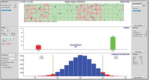
In Lesson 3, students are asked to simulate the experiment from Lesson 1 with a computer to investigate variation and uncertainty. To this end, they use a sampling distribution app from VU Stat, https://www.vustat.eu/apps/yesno/index.html. In this app, the population is displayed using colored balls, which creates a strong connection with the black box activity. In our view, the app seems user-friendly, with easy input of the population size, population proportion, and sample size. As shown in Figure 2, the software provides a clear overview of the population in the upper screen, of each individual sample result in the middle screen, and of the sampling distribution for many repetitions in the lower screen. Students simulate the sampling distribution with a large number of repetitions and use this distribution as a model for investigating most common sample results with accompanying estimates of the population. Subsequently, we expect students to use the simulated sampling distributions from a given population at varying sample sizes and at varying numbers of repetitions as a model for investigating the effect of sample size and repeated samples on the accompanying estimates of the population. Students note their findings on a student worksheet.

Figure 2. Screenshot of the VU Stat sampling distribution app (https://www.vustat.eu/apps/yesno/index.html).

The hypothesis in the third step, concerning the simulated sampling distribution, is that engaging in the designed activity makes students aware that the simulated sampling distribution can be used as a model for interpreting variation and uncertainty, and more particularly that repeated sampling with a larger sample size reduces the variation in the accompanying estimates of the population and hence leads to a more certain inference; and that sampling with a larger number of repetitions leads to less variation in the mean and hence to a better estimate of the population. The following indicators are considered as supporting the hypothesis:

• 3a) Students compare the simulated sampling distributions at varying sample sizes and note that repeated sampling with a larger sample size leads to less variation in the accompanying estimate of the population;

• 3b) Students compare the simulated sampling distributions at varying sample sizes and note that repeated sampling with a larger sample size leads to a better estimate of the population;

• 3c) Students compare the simulated sampling distributions from varying number of repetitions and note that from repeated sampling with a larger number of repetitions the mean of these samples is less variable;

• 3d) Students compare the simulated sampling distributions from varying number of repetitions and note that repeated sampling with a larger number of repetitions leads to a better estimate of the population;

• 3e) Students describe how the simulated sampling distribution from repeated sampling can be used to determine the most common sample results;

Each HLT step focuses on one key concept, in which entailing aspects – for example, sample size, repeated sampling, sampling variation, (un)certainty of an estimate, probability of samples, visualizations – are addressed from an exploratory perspective from the concrete black box in step 1 to a more abstract perspective in step 3 by simulating the sampling distribution by repeated sampling. An overview of the build-up in complexity by these aspects of ISI is displayed in Table 3.

Table 3. Overview of indicators expected in different data sources, by entailing aspects of ISI.

	HLT step 1 Sample		HLT step 2 Frequency distribution		HLT step 3 Simulated sampling distribution
Build-up in complexity	Introduction to variation and uncertainty		Visualization of variation		Interpretation of variation and uncertainty
Data source	WD1^1	SW1^2	WD2^1	SW2^2	TSI3^3	SW3^2
Sample size	1e, 1f	1e, 1f				3a, 3b
Repeated sampling	1b	1b	2a, 2b	2c, 2d	3c, 3d	3c, 3d
Sampling variation	1a		2a, 2b	2c, 2d	3a, 3b, 3c, 3d	3a, 3b, 3c, 3d
(Un)certainty of estimate of population	1c, 1d	1c, 1d, 1e				3b, 3d
Probability of particular sample results			2a, 2b	2c, 2d, 2e	3a, 3b, 3c, 3d	3a, 3b, 3c, 3d
Determination of (un) likely sample results			2a, 2b	2d	3a, 3b, 3c, 3d	3a, 3b, 3c, 3d
Use of visualization				2c, 2d, 2e	3a, 3b, 3c, 3d	3a, 3b, 3c, 3d

¹Whole-class Discussion (WD); ²Student Worksheet (SW); ³Teacher-Student Interaction (TSI)

Data collection

With respect to the first step, data included individual student worksheets filled in by students who worked in pairs with the black box and video-recordings from a 10-min whole-class discussion. In the second step, we collected data from student worksheets that were individually filled in by students and video-recordings from a 12-min whole-class discussion. For the third step, we collected data from student worksheets that were individually filled in by students who worked in pairs on a computer and eight video-recordings of 2-min interactions between teacher and students.

The video recordings were made by a research assistant and were preceded by detailed instruction on specific recording details. The worksheets of the students were distributed at the start of each lesson and collected at the end, to prevent information being added or lost.

Implementation characteristics

To empirically verify whether the three hypotheses could be confirmed, we implemented this LT in one class at a secondary school in the Netherlands. In this report, we focus on three 45-min lessons, the first three of a more extensive series of 10 lessons. We do so because this is where the students are introduced to the three key concepts by repeated sampling with the black box. The subsequent five steps of the LT, concerning seven more lessons, consist of applying these concepts in new situations with a build-up in the complexity of data.

Participants

The participants consisted of twenty 15-year-old students in Grade 9 of the pre-university level, who are among the 20% best-performing students in the Dutch education system. The 20 students formed one class with both talented and less gifted mathematics students. The students were inexperienced with sampling. They had some basic knowledge of descriptive statistics: center and distribution measures, such as mean, quartiles, class division, absolute and relative frequencies, and boxplot. The lessons were conducted during the regular mathematics lessons over a period of one week.

The teacher was the first author. In this design research, it was an advantage that the teacher-researcher was so familiar with the designed materials. This allowed all attention to be focused on the design without deviations from the designer’s intentions. Although there is added value in investigating field-based trials of an activity to see how teachers tend to implement the materials, at this stage, it is sensible to tackle challenges one by one (Tessmer, 1993).

Data analysis

To answer the research question, we analyzed the data with respect to the indicators that would support the hypotheses as formulated in the HLT. The main data sources were the student worksheets and the video recordings of both the whole-class discussions and the teacher–student interactions. Table 3 displays the distribution of the expected occurrence of indicators in the different data sources by sub-area of ISI.

Answering the how-question of our research includes design, implementation, and evaluation. To make the connection between these phases explicit, we work out indicator 1f as an illustrative example. The other indicators were elaborated in a similar way. Indicator 1f states: “Students note that working with a larger sample (usually) leads to a better estimate of the content.” In the design phase, we designed a student activity in which students collect data, analyze their data, and formulate an inference on the basis of a given investigation question. The activity concerns the context of a black box experiment and is built up according to the educational ideas of repeated and growing samples. The full HLT incorporated a detailed description of the designed activity, including all implementation issues involved. During the implementation phase in lesson 1, students worked on the designed activity in pairs and noted their data collection and data analysis, as well as their inference (estimate of the content) along with an indication of their (un)certainty, on their worksheet as an answer to tasks 1–3 (Table 4). In the following whole-class discussion, the results were exchanged and discussed. Subsequently, the teacher posed the question: “What happens if we enlarge the viewing window?” Different options were exchanged and discussed, with attention to the uncertainty involved. After the whole-class discussion, students doubled the sample size (larger window) of their black box and again collected data, analyzed these and made a new inference with an indication of their (un)certainty, and noted the results on their worksheet as an answer to tasks 4–6. After that, students were asked in task 7 on the student worksheet to compare their answers for tasks 1–6 and draw a conclusion about the effect of sample size on the estimate of the content. During the analyses, we used data from tasks 1–7 on the student worksheets and video data of the whole-class discussion. The data analysis of these sources is elaborated on below.

Table 4. Overview of results for LT step 1.

Indicators	Student worksheet (N = 20) (observed number of students)	Video (strong, weak, no evidence)
1a. Students note that their sample results vary	Non-applicable	Strong
1b. Students choose a repeated sampling approach, with calculating the average, to estimate the number or proportion of yellow balls	n = 20	Strong
1c. Students note that it is possible to estimate the content based on samples	n = 20	Strong
1d. Students note that it is impossible to determine the exact content based on samples	n = 20	Strong
1e. Students note that the larger the sample size, the more confident they are on their estimate	n = 17	Strong
1f. Students note that working with a larger sample (usually) leads to a better estimate of the content	n = 20	Strong

All video data, both whole-class discussions and teacher–student interactions, were transcribed and coded. The codebook consisted of the indicators in Table 3. The unit of analysis during the discussions and interactions was a central question brought forward by the teacher to check out the indicators, and the corresponding reactions by the students. For example, a central question in the discussion of step 1 was “What do you know for sure about the number of yellow balls in the black box?” which refers to indicators 1c and 1f. To distinguish clear instances and less clear instances, the evidence was coded as strong, weak or no evidence. Strong evidence refers to indicators that were explicitly present during the class discussion or interaction, for example, conclusions that were expressed literally or assumptions that were used and repeated more than once. Weak evidence refers to indicators that were partly observed, for example, incomplete conclusions or assumptions discussed indirectly. No evidence refers to indicators that were attended during the discussion but were not confirmed or contradicted.

Student worksheets were coded according to the same codebook. The worksheets consisted of structured and open tasks. For the analysis, only open tasks were used in which students were explicitly asked to clearly motivate their answer. The worksheets contained specific tasks that were directly related to the indicators. For example, task 6 (“Are you sure of your estimate from a larger sample?”) and 7 (“What did you learn from a larger sample?”) on Worksheet 1 refer to indicators 1d and 1e, respectively. The frequency with which each indicator was coded was noted.

Indicators that were not attended to during the whole-class discussion or on the worksheet were indicated as “non-applicable.” A second coder was used to analyze the video data of the whole-class discussions and the teacher–student interactions, as well as the answers to open tasks on the worksheets. A random sample of 25% of the data was checked by the second coder. Cohen’s kappa was .83, indicating a good interrater reliability.

Results

For each hypothesis, this section describes whether the supporting indicators were observed.

First step: sample

The hypothesis in the first step, introducing the concept of a sample, was confirmed as the indicators 1a to 1f were coded in the data collected. Table 4 displays the observed indicators.

The strategies for investigating the number of yellow balls in a black box with a small viewing window that students showed on their worksheet, corresponded to indicator 1a to 1d. Table 5 gives an overview of these results on Worksheet 1 on small samples from the black box.

Table 5. Answers on worksheet 1 on small samples (size 20) from the black box (N = 20, number of students).

Task	Students’ answers	Examples from written work
1. Estimate the number of yellow balls in the black box.	682, 750, 750, 625, 700, 730, 700, 735, 700, 725, 750, 675, 675, 730, 750, 725, 682, 733, 700, 625 (estimate of each student) (n = 20).
2. Explain your estimate.	Approach 1: count balls, calculate average, convert to the contents of the entire box (n = 14).	We took 10 samples with 20 balls, calculated the average and multiplied this by 50.
	Approach 2: estimate the ratio of yellow balls after shaking a few times and convert to the entire box (n = 6).	Always around 15–16 yellow and the remaining orange.
3. How confident are you about your estimate?	Not confident (n = 2). Quite confident (n = 16). Most confident (n = 2).	Not sure, just guessing. We don’t know exactly, but it’s about this number. Most confident, but not 100% sure, because we calculated the averages and extrapolated this number to the content.

As a first strategy, after shaking up the box to mix the objects, most students (14 out of 20) counted the visible yellow balls in the viewing window and extrapolated this number into the total content. They then repeated this shaking and counting five to ten times and used the average of these counts to estimate the content. This strategy was also expressed during the whole-class discussion, in which Ruben (all names are pseudonyms) added the following:

Teacher:

How did you get the estimate?

Joerie:

We counted the number of yellow balls and counted the total number of balls in the window. Then we converted the numbers into the total content. We repeated this about ten times and then calculated the average.

Teacher:

Are there students with a different approach?

Ruben:

Well, about the same thing, but we counted the orange balls, there are less of them, and then converted to the total. We repeated this about seven times and calculated the average.

As a second strategy, after shaking up the box, some students (6 out of 20) based their estimate not on counts, but on ratios. For example, one of these students indicated: “We have shaken the black box several times and there are always about 15–16 yellow balls and the remaining ones are orange.” All students decided to shake and measure several times, which showed that the students were confronted with sampling variation when estimating the content and opted for repeated sampling to get a better estimate. The students’ estimates ranged from 625 to 750. Most students were quite confident about their estimate. Only two students indicated that it was a guess and two students were most confident – although not 100% sure – because their estimate was based on a calculation with the average from multiple counts.

As a follow-up activity, students worked with a larger viewing window. Most students were more confident about their estimate based on a larger window, and all students noted that a larger window led to a better estimate of the content, which corresponded to indicators 1e and 1f. Table 6 provides an overview of these results with students’ answers on Worksheet 1 with larger samples from the black box.

Table 6. Answers on worksheet 1 with large samples (size 40) from the black box (N = 20).

Task	Students’ answers	Examples from written work
4. Estimate the number of yellow balls in the black box.	744, 750, 714, 720, 720, 730, 720, 728, 725, 725, 750, 731, 731, 730, 714, 725, 744, 728, 725, 720 (estimate of each student) (n = 20).
5. Explain your estimate.	Approach 1: count balls, calculate average, convert to the contents of the entire box (n = 20).
6. Are you confident about your estimate from a larger sample?	More confident than before, with the small window (n = 17).	More sure because the estimates are now less variable. More sure because you have more information.
	Still not confident (n = 3).	Not sure yet because the results still vary.
7. What did you learn from a larger sample?	A larger sample size gives a better estimate (n = 20).	A larger sample gives more information about the content.

With this larger window, all students used the first strategy of counting the number of yellow balls several times and converting the average to the entire content. This time students’ estimates showed less variation, as they ranged from 714 to 750. Most students (17 out of 20) wrote that they were more confident of their estimate based on this larger sample. Some students mentioned in this respect: “We are more confident because the estimates are now less variable,” and others quoted: “More sure because you have more information.” Three students wrote that they were not confident because the sample results still varied. However, these three did indicate in the next task that the best way to estimate the content was to use a larger sample.

Although the students initially gave a numerical value as an estimate of the total number of balls, they later switched to an interval, which revealed indicators 1c and 1d. This transition became clearly visible during the discussion when the teacher explicitly asked: “What do you know for sure about the number of yellow balls in the black box?”

Daphne:

Well, that three-quarters of the balls are yellow, and one-quarter are orange.

Teacher:

Are you sure about the three-quarters?

Daphne:

Yes, a bit more or less, because…. Yes, there are more yellow balls than orange balls.

Bas:

I think the number of yellow balls is around, uhm, 700. It may be little less. In any case, it is between the 625 and 750.

Jesse:

Yes, it is in any case between 600 and 800.

Here, Bas took the extreme values of the observed samples as limits for the possible number of yellow balls. Jesse took a broader interval. Both showed that they understood that sample results vary, but can be used to estimate the population. Jesse’s reply indicated that he understood that these extreme values were global estimators that might vary due to chance.

Second step: frequency distribution

Regarding the second step, introducing the concept of frequency distribution, the hypothesis was confirmed. The results showed that indicators 2a to 2e were observed. Table 7 displays the observed indicators.

Table 7. Overview of results for LT step 2.

Indicators		Student worksheet (N = 20) (observed number of students)	Video (strong, weak, no evidence)
2a. Students note that sample results corresponding to the population proportion will often occur;		Non-applicable	Strong
2b. Students note that strongly deviating sample results are unlikely to appear;		Non-applicable	Strong
2c. Students sketch a graph of the frequency distribution with a top at the population proportion (in this case 30);		n = 20	Non-applicable
2d. Students sketch a graph of the frequency distribution in which the extreme values (in this case 0–10 and 35–40) hardly occur;		n = 20	Non-applicable
2e. Students estimate the probability of ranges of particular sample results on the basis of their sketched frequency distribution^1,2,3;		n = 12	Non-applicable
	^1Supplement: Students estimate the probability of ranges of particular sample results roughly	n = 20	Non-applicable
	^2Supplement: Students estimates did not correspond to their frequency distribution sketched	n = 7	Non-applicable
	^3Supplement: Students overestimated the probability of strongly deviating results	n = 6	Non-applicable

The whole-class discussion focused on the question “What happens if this experiment is repeated?” Students mentioned that results that resembled the population proportion were most likely to appear and that strong deviations were unlikely but possible, which confirmed the expected students’ behavior as described in 2a and 2b. However, it seemed that some students overestimated the possibility of strongly deviating results, as they suspected that with a large number of repetitions there would certainly be outliers. At the same time, students seemed to become aware of the difference between possibility and chance, which followed from the next interview fragment.

Teacher:

What sample result is unlikely?

Iris:

Eh, that all the balls are orange.

Bas:

That is possible, though there are more than 40 balls in the box.

Iris:

Yes, but little chance that this will happen.

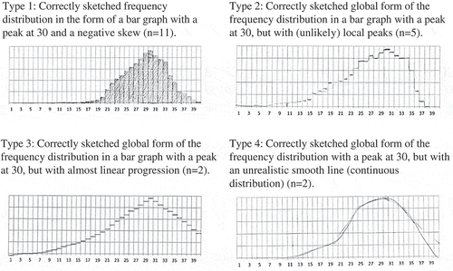
All students were able to understand the frequency distribution of data from repeated sampling, as they made a good sketch of a visualization (or a model) of their expectations in a distribution with a peak at 30 and falling to (almost) zero at the extremes, which corresponded to indicators 2c and 2d. In doing so, all students demonstrated that they were aware that samples vary, but that a sample result that resembled the population proportion (75%) would occur most frequently in more than 100,000 repetitions. The drawings could be divided into the four types shown in Figure 3. Eleven students correctly sketched the frequency distribution in the shape of a bar diagram with a peak at 30 and a negative skew (Type 1). Five students indicated that for so many repeated samples, the sample results would not increase/decrease monotonously, but local peaks might occur (Type 2). These five students also correctly sketched the global features of the frequency distribution, although local peaks are unlikely to occur in such a large number of repetitions. These students probably thought that coincidence played a role in this, and they did not (yet) realize that the distribution of samples will stabilize after so many repeated samples (known as the law of large numbers, which we do not expect students to understand here). Two students sketched an almost linear course (Type 3) and two students outlined a smooth curve (Type 4). However, the latter might be caused by the word sketch rather than draw in the task.

Figure 3. Four types of students’ sketches (N = 20) of the expected results of repeated sampling (100,000 repetitions) with sample size 40 in a frequency distribution.

Students were able to estimate the probability of certain sample results roughly, but their estimates did not always correspond to their sketched frequency distribution and some students overestimated the probability of strongly deviating results, and, as a consequence, indicator 2e was only partially observed. In several tasks, students were asked to estimate the probability of ranges of particular sample results. As an example, Table 8 shows the results of one task, in which students were asked to estimate the probability of a sample result of less than 10 in a sample of 40 from a population (size 1,000 and proportion 75%).

Table 8. Students’ estimate of the probability of a range of particular sample result on worksheet 2 (N = 20).

Task	Probability	Examples of written work
1. How do you estimate the probability of a sample result (amount of yellow balls) of less than 10 at a sample size of 40? (population proportion 75%)	(Almost) 0% (n = 6)	Very small, but it is possible though.
	1% (n = 6)	A very small probability actually, almost 1%, because there are simply many more yellow than orange balls.
	5% (n = 3)	.. because there will always be a chance, only it gets less because the larger majority has that color.
	10% (n = 3)	75 out of 100 balls are yellow.
	Empty (n = 2)	(due to time limitations)

Although it was expected that students would describe their estimate of the probability in words, students apparently felt the need to quantify it (probably because this activity was part of the mathematics lesson) and chose to use percentages. All students estimated the probability of a sample result under 10 less than or equal to 10%, with only 6 out of 20 students estimating this probability close to zero. These answers demonstrated that students understood that the probability of a strongly deviating result was small. However, this probability was overestimated as six of them indicated that it would be 5% or higher.

A remarkable result in determining the probability of ranges of particular sample results was that the frequency distribution sketched by the students did not always correspond to their answers (7 out of 20). Table 9 shows an example. Although this student wrote down a numerical value, suggesting that he made a calculation or at least made a specific estimate from his sketch, the value did not match his sketched frequency distribution. It seemed that the estimate was based on his intuitive idea of probability rather than being calculated or estimated using his frequency distribution. However, two other students explicitly mentioned that they did calculate the probability, “I estimate the probability at 0.01% which is about 10 out of 100,000 times.” In this case, the calculation shown was the basis for the correct reasoning.

Table 9. Illustrative example of the working method on worksheet 2.

Task	Illustrative example from one student’s work
Sketch the expected frequency distribution on the number of yellow balls in a sample of 40, if the first-step physical experiment were repeated 100,000 times. (population proportion 75%)
How do you estimate the probability of a sample result (amount of yellow balls) of less than 10 at a sample size of 40? (population proportion 75%)	I estimate the probability at 10%, because most balls are yellow.

Third step: simulated sampling distribution

With regard to the third step, introducing the concept of the simulated sampling distribution, the hypothesis was confirmed as the data analysis revealed indicators 3a to 3e. Table 10 displays the observed indicators.

Table 10. Overview of results for LT step 3.

Indicators	Student worksheet (N = 20) (observed number of students)	Video (strong, weak, no evidence)
3a. Students compare the simulated sampling distributions at varying sample sizes and note that repeated sampling with a larger sample size leads to less variation in the accompanying estimate of the population;	n = 20	Strong
3b. Students compare the simulated sampling distributions at varying sample sizes and note that repeated sampling with a larger sample size leads to a better estimate of the population;	n = 20	Strong
3c. Students compare the simulated sampling distributions from varying number of repetitions and note that from repeated sampling with a larger number of repetitions, the mean of these samples is less variable;	n = 20	Strong
3d. Students compare the simulated sampling distributions from varying number of repetitions and note that repeated sampling with a larger number of repetitions, leads to a better estimate of the population;	n = 20	Strong
3e. Students describe how the simulated sampling distribution from repeated sampling can be used to determine most common sample results;	Non-applicable	Weak

The students were able to simulate the sampling distributions at varying sample sizes and from a varying number of repetitions and to use these distributions as a model for interpreting the variation and uncertainty involved. By comparing these distributions, they noted on their worksheet that a larger sample size leads to less variation in the accompanying estimate of the population and hence to a better inference, and in addition they noted on their worksheet that a larger number of repetitions lead to less variation in the mean of the samples and hence to a better estimate of the population, which confirmed indicators 3a to 3d.

The students could simulate the sampling distributions from repeated sampling easily and independently. They determined the most common sample results for samples with different sizes and different number of repetitions by checking the boundaries of the 95% area with the computer tool. This tool also made it easy to determine the average sample result. Students were asked to examine the effect of sample size and the number of repetitions on the sampling distributions. In order to investigate this, they could use the tables on their worksheet. Figure 4 displays one filled-in table of a student.

Figure 4. Example of filled-in table on Worksheet 3

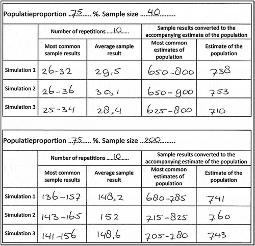
The students were free to decide which population proportion, sample size, and the number of repetitions they wanted to examine and compare. Based on the simulated sampling distributions, they filled in Columns 2 and 3 and subsequently converted these values to the accompanying estimates of the population (size 1,000) in Columns 4 and 5.

By comparing sampling distributions with different sample sizes, students noted that there was less variation in the corresponding estimates of the population and concluded that a larger sample size led to a more accurate outcome. Table 11 gives an overview of students reasoning about the effect of sample size on the estimate of the population. In the same way, students compared simulated sample distributions for a varying number of repetitions and found that the average sample result for a large number of repetitions remained almost the same, and from this, they concluded that more repeated samples provided a better estimate of the population.

Table 11. Students’ estimate of the probability of a certain sample result on worksheet 2 (N = 20).

Task	Examples from written work
1. What do you notice when you compare the population estimates from a small sample size with those from a larger one?	The estimates from a larger sample size are closer together. With a larger sample size, the average sample result, and the population estimate, are closer together. With a larger sample size, there is less variation in the population estimates.
2. Based on the simulated sample distributions, draw a conclusion on the effect of sample size on the estimate of the population. Complete the following sentence: A larger sample size …	… leads to a more accurate conclusion. … gives a more precise picture of the number in the population. … reduces the spread of the estimates, which in turn makes your estimate of the population more precise.

Since most students used the boundaries of the 95% to compare the sampling distributions, the teacher asked several individual students what these boundaries meant and how one could use them. These videotaped interactions between teacher and student (TSI) showed that the students’ overall idea of the 95% area was correct. For example, based on the screen with the 95% area of the sampling distribution one student explained:

The 95% area consist of two borders, a limit at 2.5% and a limit at 97.5% of the sample results. This is so that you can clearly see what the most common sample results are. The sampling variation is sometimes very large because you carry out many samples. Through the 95% area you can see clearly what the samples usually have as a result.

Not all students were surveyed, and the open nature of the question made it hard to confirm their understanding of the 95% area; as a consequence, we considered indicator 3e as partly observed, even though all students were able to describe how the sampling distribution could be used as a model to interpret variation and uncertainty and to determine most common sample results.

Conclusion and discussion

In this research, we looked for opportunities to make ISI accessible to ninth-grade students. Educational guidelines were extracted from literature and translated into hypotheses about a learning trajectory for students. We addressed the question of how the first part of a learning trajectory that focuses on repeated sampling with a black box introduces students to the concepts of sample, frequency distribution, and simulated sampling distribution. This article reports on the design, implementation, and evaluation of the first three steps of an LT for ISI.

The first step of the LT focused on the introduction of sampling. The hypothesis was that students would become aware of sampling variation with categorical data and investigate the effect of repeated sampling and sample size on estimating the population, by conducting the designed activity with the black box. The results show that the indicators associated with the hypothesis were observed. The LT enabled students, inexperienced with sampling, to reason with sample data in a short period of time, including the handling of variation and uncertainty. To estimate the population – the content of the black box – students chose a repeated sampling approach to reduce errors caused by sampling variation. In this specific black-box context, students viewed their sample as “a subset of the population” and not as “a small-scale version of the population” which supports reasoning about variation (Saldanha & Thompson, 2002). Students did not know how to interpret the variation in data, as they noted that they were not entirely confident about their estimates due to the variation in outcomes. This result is in line with studies by Tversky and Kahneman (1971) and Ben-Zvi et al. (2012). The use of whole-class discussions where students exchange and compare their results from repeated sampling (Wild & Pfannkuch, 1999), along with the growing-samples principle (Bakker, 2004; Ben-Zvi et al., 2012), in which students discuss and test their expectations about increasing sample sizes, was found transportable to our LT. Along the lines of this approach, students predicted what would happen in the following larger sample. While drawing larger samples and exchanging the results, the role of sample size on variation became visible for students. Students experienced and noted that a larger sample size (usually) leads to less variation in the estimate of the population proportion and hence to a better inference. The confrontation with diversity in sample data from the black box supported students’ inferential reasoning about the boundaries of variation. Estimates of the population proportions were supported by arguments on sampling variation, repeated sampling, and sample size. As such, this physical black-box experiment seemed a meaningful context to introduce students to the concept of sampling.

The second step of the LT focused on the introduction of the concept of frequency distribution from repeated sampling. The hypothesis was that for students the frequency distribution was primarily a visualization of results obtained from repeated samples. Through considering how this distribution might look like with many repeated samples, students were stimulated to make the conceptual switch to using it as a model for interpreting variation and uncertainty. Along this way, it was expected that during this step, through discussing the question “What happens if this experiment is repeated,” and by imagining and visualizing the frequency distribution of 1,000 repeated samples from the black box, students would understand that most sample results will be close to the population proportion and that strong deviations are unlikely. In addition, they were expected to understand that this frequency distribution can be used to estimate the probability of ranges of specific sample results (for example, a result of less than 10). The results from step 2 show that most of the corresponding indicators were observed. The question of what happens if the experiment is repeated (Rossman, 2008) was found crucial in this LT. It promoted students’ inferential reasoning as they considered and discussed possible sample results. Moreover, this question led to a discussion about the difference between probability and chance. By having students draw a sketch of their expectations for many repeated samples in a bar chart, the shape of frequency distribution became visible.

This visualization offered a lead to more enhanced reasoning about variation and uncertainty. As all students were able to consider, sketch, and reason about variation and uncertainty with the frequency distribution on repeated sampling, students were expected to be able to determine the probability of ranges of particular sample results by using their prior knowledge of ratios. However, as a remarkable result, not all students applied their prior knowledge of ratios to their sketched frequency distribution; some determined the probability on other (maybe more intuitive) ideas. Another finding in this respect is that some students overestimated the probability of strong deviations, which is not surprising at this stage but can be a point for attention in subsequent lessons. From these results, visualizing the expected frequency distributions on many repeated samplings facilitated more enhanced reasoning about variation and uncertainty, where determining the probability of particular sample results is a point for attention.

The third step focused on the introduction of the concept of sampling distribution. The hypothesis was that students would understand that this distribution can be used as a model for investigating variation and uncertainty. More particularly, that students understand that sampling with a larger number of repetitions leads to less variation in the mean and hence to a better population estimate, and that sampling with a larger sample size reduces the variation in the accompanying estimates of the population and hence leads to a more certain inference, by simulating and comparing sampling distributions with varying sample sizes and from varying number of repetitions. The results of step 3 show that the indicators that supported the hypothesis were observed. From students’ experience with the frequency distribution of many repeated samples in step 2, the transition to the simulation of the sampling distribution, also called resampling (Garfield et al., 2015; Manor & Ben-Zvi, 2015; Watson & Chance, 2012), was easily made. The students were already familiar with the shape of this distribution. The students were able to determine the most likely sample results by using the digital tool. Here they used the boundaries of the 95% area, which were available in the tool. The students simply adopted these boundaries. Although most students were able to give a correct description of these boundaries, the results do not confirm whether all students understood these boundaries and their application. The comparison of distributions from repeated sampling gave them insight into the effect of repeated sampling and sample size on the estimate of the population. As such, the results show that students were able to use the idea of a simulated sampling distribution as a model for further investigating variation and uncertainty.

This study gave an insight into how an LT that focuses on the concept of sample, frequency distribution, and sampling distribution can enhance ninth-grade students’ informal inferential reasoning. The results show how students used these concepts to underpin their inferences, especially with regard to variation and uncertainty. In addition, the results show what barriers students encountered during their work on the HLT.

From the viewpoint of the researcher as an experienced teacher, the main element in this LT that allowed students to go through the three steps smoothly seemed to be the accessibility of the three successive steps. From their concrete experiences with sampling variation in step 1, through imagining and visualizing the scaling up of this experiment in step 2, the students could easily make the transition to reasoning with the sampling distribution in step 3. From their point of view, the computer took over their manual work. This approach provided them insight into how the sampling distribution arises and how it can be used as a model for investigating possible sample results to interpret variation and uncertainty. Known difficulties concerning the three main concepts of sample, frequency distribution, and sampling distribution, hardly occurred and apparently were avoided. As a consequence, this approach seems to help students engage with these concepts, which supports them in using new insights in new situations, making ISI accessible.

In our study, the idea of model of to model for was primarily used as a design heuristic to promote emergent modeling (Gravemeijer, 1999). In retrospect, we have become intrigued by what happens cognitively when students make the transition from seeing a graph as a representation (model) of a frequency distribution to seeing a dataset as a distribution with particular characteristics that help to make inferences (model for). It seems promising to analyze such transitions through the theoretical lens of objectification (reification, reflective abstraction, or hypostatic abstraction). Where it concerns the learning of function (Sfard, 1991), it is known that students initially see functions as processes, and typically not as objects with characteristics. The desired dual understanding of functions or other mathematical objects as both process- and object-like has been referred to as “procept” (Gray & Tall, 1994). In our case, we speculate that the sampling process in which students see (sampling) distributions emerges may be such a process view, which forms a basis for seeing a distribution as an object (cf. Bakker, 2007b). From such a perspective, the question arises whether objectification is indeed the mechanism that enables the cognitive transition between the learning steps, and thus conceptualization.

Objectification involves constructing an object in a representational system, for example, the visualization of a sample, experimenting with this object and then observing the results of experimenting, as a reflection phase. New objects can be created in the reflection phase when part of an object is seen as an entity in itself (Bakker, 2007a). The central point of this reflection phase is that the new objects formed by this process can be used as a means for further objectification, for new, higher-level processes, and for further steps in improving additional knowledge, and thus conceptualized as an independent entity. According to Sfard and Lavie (2005), the development of objectification begins with participation in offered routines with the object, whereby these routines gradually transform into real explorations with the object as an independent entity. They emphasize that this learning process is a one-way street, which is difficult to reverse, making it hard for adults to recognize. With regard to the transfer from LT step 1 to step 2, objectification may involve the transfer of sampling as the process of creating elements of a dataset, to a sample as an element or new object in the frequency distribution from repeated samples in step 2. In this way, objectification can be viewed as the mechanism underlying the ideas of repeated and growing samples. With regard to the transfer from LT step 2 to 3, objectification may facilitate the transfer of the frequency distribution as a model of results generated from repeated sampling into a model for further investigating variation and uncertainty. Given the importance of such a mechanism of objectification, we recommend follow-up research in this area.

Our advice for the redesign of the HLT focuses on two main points. The first point includes the integration of students’ prior knowledge about proportions to determine the probability of ranges of particular sample results with the frequency distribution. This could be achieved by calculating proportions by using (and discussing possible) units on the vertical axis of the (expected) frequency distribution and by applying and discussing this distribution in multiple and more different situations. The second point for the redesign is to pay more attention to reasoning with the simulated sampling distribution in various situations and not automatically use the 95% area. Discussion on students’ analyses and not only on the results will support students’ development of strong mathematical arguments (McClain, McGatha, & Hodge, 2000).

Considerations for using the LT in other settings are the following. The LT was implemented in the classroom of the teacher-researcher, who was very familiar with the class and the designed materials. We are aware that this favorable condition should be taken into account when readers want to use the ideas presented here in other contexts. Researchers who would like to repeat such activities should also consider that most Dutch students are not used to whole-class discussions during the mathematics lessons. In our research, it was important to encourage them to reason and discuss with each other from the beginning of the trajectory. Teachers and researchers should also take into account that Dutch students are used to closed assignments from their textbook and are unfamiliar with working with more open and inquiry-based tasks. Another point of consideration is that we worked with pre-university students, the top 20% of our education system. In other situations, students may need more time. As the results in this research are based on a small-scale pilot in the class of the teacher-researcher, these results are not generalizable to a regular classroom without further research.

This research that focused on repeated sampling with the black box as the first part of an LT seems a promising proof of principle how to make ISI – e.g., reasoning about variation and uncertainty – accessible for students along the lines of sample, frequency distribution, and simulated sampling distribution. The results of this study will be used to revise the first part of the LT, and as a next step, in a follow-up study, to (re)design the whole LT, and to improve effectiveness, efficiency, scale up and compare our HLT with alternatives.

Additional information

Funding

This research received funding from the Ministry of Education, Culture and Science under the Dudoc program.

References

- Ainley, J., Pratt, D., & Hansen, A. (2006). Connecting engagement and focus in pedagogic task design. British Educational Research Journal, 32(1), 23–38. doi:10.1080/01411920500401971
- Bakker, A. (2004). Design research in statistics education. On symbolizing and computer tools. Utrecht, the Netherlands: Utrecht University.
- Bakker, A. (2007a). Diagrammatic reasoning and hypostatic abstraction in statistics education. Semiotica, 164, 9–29. doi:10.1515/SEM.2007.017
- Bakker, A. (2007b). Diagrammatisch redeneren als basis voor begripsontwikkeling in het statistiekonderwijs [Diagrammatic reasoning as a basis for concept development in statistics education]. Pedagogische Studiën, 84(5), 340–357.
- Ben-Zvi, D. (2006). Scaffolding students’ informal inference and argumentation. In A. Rossman & B. Chance (Eds.), Proceedings of the Seventh International Conference on Teaching Statistics. [CD-ROM]. Voorburg, the Netherlands: International Statistical Institute.
- Ben-Zvi, D., Aridor, K., Makar, K., & Bakker, A. (2012). Students’ emergent articulations of uncertainty while making informal statistical inferences. ZDM the International Journal on Mathematics Education, 44(7), 913–925. doi:10.1007/s11858-012-0420-3
- Ben-Zvi, D., Bakker, A., & Makar, K. (2015). Learning to reason from samples. Educational Studies in Mathematics, 88(3), 291–303. doi:10.1007/s10649-015-9593-3
- Castro Sotos, A. E., Vanhoof, S., van Den Noortgate, W., & Onghena, P. (2007). Students’ misconceptions of statistical inference: A review of the empirical evidence from research on statistics education. Educational Research Review, 1(2), 90–112.
- Chance, B., Ben-Zvi, D., Garfield, J., & Medina, E. (2007). The role of technology in improving student learning of statistics. Technology Innovations in Statistics Education Journal, 1(1), 1–23.
- Clements, D. H., & Sarama, J. (2004). Learning trajectories in mathematics education. Mathematical Thinking and Learning, 6(2), 81–89. doi:10.1207/s15327833mtl0602_1
- Doerr, H., delMas, R., & Makar, K. (2017). A modeling approach to the development of students’ informal inferential reasoning. Statistics Education Research Journal, 16(2), 86–115.
- Franklin, C., Kader, G., Mewborn, D., Moreno, J., Peck, R., Perry, M., & Schaeffer, R. (2007). Guidelines for assessment and instruction in statistics education (GAISE) report. Alexandria, United States: American Statistical Association.
- Gal, I. (2002). Adults’ statistical literacy, meanings, components, responsibility. International Statistical Review, 70(1), 1–51. doi:10.1111/j.1751-5823.2002.tb00336.x
- Garfield, J., Ben-Zvi, D., Le, L., & Zieffler, A. (2015). Developing students’ reasoning about samples and sampling variability as a path to expert statistical thinking. Educational Studies in Mathematics, 88(3), 327–342. doi:10.1007/s10649-014-9541-7
- Gravemeijer, K. (1999). How emergent models may foster the constitution of formal mathematics. Mathematical Thinking and Learning, 1, 155–177. doi:10.1207/s15327833mtl0102_4
- Gravemeijer, K. P. E., Bowers, J., & Stephan, M. L. (2003). A hypothetical learning trajectory on measurement and flexible arithmetic. Journal for Research in Mathematics Education, 12, 51–66.
- Gray, E. M., & Tall, D. O. (1994). Duality, ambiguity, and flexibility: A “proceptual” view of simple arithmetic. Journal for Research in Mathematics Education, 25(2), 116–140. doi:10.2307/749505
- Innabi, H., & El Sheikh, O. (2007). The change in mathematics teachers’ perceptions of critical thinking after 15 years of educational reform in Jordan. Educational Studies in Mathematics, 64(1), 45–68. doi:10.1007/s10649-005-9017-x
- Konold, C., & Kazak, S. (2008). Reconnecting data and chance. Technology Innovations in Statistics Education, 2(1), Article 1.
- Konold, C., & Pollatsek, A. (2002). Data analysis as the search for signals in noisy processes. Journal for Research in Mathematics Education, 33(4), 259–289. doi:10.2307/749741
- Lehrer, R., & English, L. D. (2017). Introducing children to modeling variability. In D. Ben-Zvi, J. Garfield, & K. Makar (Eds.), International handbook of research in statistics education (pp. ADD). Dordrecht, the Netherlands: Springer.
- Makar, K. (2016). Developing young children’s emergent inferential practices in statistics. Mathematical Thinking and Learning, 18(1), 1–24. doi:10.1080/10986065.2016.1107820
- Makar, K., Bakker, A., & Ben-Zvi, D. (2011). The reasoning behind informal statistical inference. Mathematical Thinking and Learning, 13(1–2), 152–173. doi:10.1080/10986065.2011.538301
- Makar, K., & Rubin, A. (2009). A framework for thinking about informal statistical inference. Statistics Education Research Journal, 8(1), 82–105.
- Manor, H., & Ben-Zvi, D. (2015). Students’ articulations of uncertainty in informally exploring sampling distributions. In A. Zieffler & E. Fry (Eds.), Reasoning about uncertainty: Learning and teaching informal inferential reasoning (pp. 57–94). Minneapolis, United States: Catalyst Press.
- McClain, K., McGatha, M., & Hodge, L. (2000). Improving data analysis through discourse. Mathematics Teaching in the Middle School, 5(8), 548–553.
- McKenney, S., & Reeves, T. C. (2012). Conducting educational design research. London. United Kingdom/New York, NY: Routledge.
- Meletiou-Mavrotheris, M., & Paparistodemou, E. (2015). Developing young learners’ reasoning about samples and sampling in the context of informal inferences. Educational Studies in Mathematics, 88(3), 385–404. doi:10.1007/s10649-014-9551-5
- Paparistodemou, E., & Meletiou-Mavrotheris, M. (2008). Developing young students’ informal inference skills in data analysis. Statistics Education Research Journal, 7(2), 83–106.
- Pfannkuch, M. (2011). The role of context in developing informal statistical inferential reasoning: A classroom study. Mathematical Thinking and Learning, 13(1–2), 27–46. doi:10.1080/10986065.2011.538302
- Pfannkuch, M., Ben-Zvi, D., & Budgett, S. (2018). Innovations in statistical modelling to connect data, chance and context. ZDM Mathematics Education, 50, 1113–1123. (online). doi:10.1007/s11858-018-0989-2.
- Rossman, A. J. (2008). Reasoning about informal statistical inference: One statistician’s view. Statistics Education Research Journal, 7(2), 5–19.
- Saldanha, L. A., & Thompson, P. W. (2002). Conceptions of sample and their relationship to statistical inference. Educational Studies in Mathematics, 51(3), 257–270. doi:10.1023/A:1023692604014
- Sandoval, W. A. (2014). Conjecture mapping: An approach to systematic educational design research. Journal of the Learning Sciences, 23(1), 18–36. doi:10.1080/10508406.2013.778204
- Sfard, A. (1991). On the dual nature of mathematical conceptions: Reflections on processes and objects as different sides of the same coin. Educational Studies in Mathematics, 22(1), 1–36. doi:10.1007/BF00302715
- Sfard, A., & Lavie, I. (2005). Why cannot children see as the same what grown-ups cannot see as different? Early numerical thinking revisited. Cognition and Instruction, 23(2), 237–309. doi:10.1207/s1532690xci2302_3
- Simon, M. A. (1995). Reconstructing mathematics pedagogy from a constructivist perspective. Journal for Research in Mathematics Education, 26(2), 114–145. doi:10.2307/749205
- Simon, M. A., & Tzur, R. (2004). Explicating the role of mathematical tasks in conceptual learning: An elaboration of the hypothetical learning trajectory. Mathematical Thinking and Learning, 6(2), 91–104. doi:10.1207/s15327833mtl0602_2
- Tessmer, M. (1993). Planning and conducting formative evaluation. London, United Kingdom: Kogan Page.
- Thijs, A., Fisser, P., & Van der Hoeven, M. (2014). 21e-eeuwse vaardigheden in het curriculum van het funderend onderwijs [21st century skills in the curriculum of fundamental education]. Enschede, the Netherlands: SLO.
- Tversky, A., & Kahneman, D. (1971). Belief in the law of small numbers. Psychological Bulletin, 76(2), 105–110. doi:10.1037/h0031322
- Van Dijke-Droogers, M., Drijvers, P., & Tolboom, J. (2017). Enhancing statistical literacy. In T. Dooley & G. Gueudet (Eds.), Proceedings of the Tenth Congress of the European Society for Research in Mathematics Education (CERME10, February 1 –5,2017) (pp. 860–867). Dublin, Ireland: DCU Institute of Education and ERME.
- Van Dijke-Droogers, M. J. S., Drijvers, P. H. M., & Bakker, A. (2018). Repeated sampling as a step towards informal statistical inference. In M. A. Sorto, A. White, & L. Guyot. (Eds.), Looking back, looking forward. Proceedings of the Tenth International Conference on Teaching Statistics (ICOTS10, July, 2018), Kyoto, Japan. Voorburg, The Netherlands, International Statistical Institute.
- Van Streun, A., & Van de Giessen, C. (2007). Een vernieuwd statistiekprogramma: Deel 1 [A renewed statistical programme, part 1]. Euclides, 82(5), 176–179.
- Watson, J., & Chance, B. (2012). Building intuitions about statistical inference based on resampling. Australian Senior Mathematics Journal, 26(1), 6–18.
- Wild, C. J., & Pfannkuch, M. (1999). Statistical thinking in empirical enquiry. International Statistical Review, 67(3), 223–265. doi:10.1111/j.1751-5823.1999.tb00442.x
- Wild, C. J., Pfannkuch, M., Regan, M., & Horton, N. J. (2011). Towards more accessible conceptions of statistical inference. Journal of the Royal Statistical Society: Series A (Statistics in Society), 174(2), 247–295. doi:10.1111/rssa.2011.174.issue-2
- Zieffler, A., Garfield, J., delMas, R., & Reading, C. (2008). A framework to support research on informal inferential reasoning. Statistics Education Research Journal, 7(2), 40–58.