Accounting and governance risk forecasting in the health care industry

Abstract

Previous authors have proved the advantage of commercial Accounting and Governance Risk (AGR) evaluation methods over academic methods. However, the information used in commercial methods is not readily available to an investor. Therefore, the most important features used in academic methods and the AGR was forecast by Random Forests. It found a weak relation between the AGR rating and share price data (Close and Volume), using a skew t-distribution. For visualisation we used the Kohonen map, which identified three clusters. Clusters revealed AGR increasing, decreasing trendsetting and cluster-based companies which appear to have no clear trend. A self-organised map (SOM) used the AGR history of alpha-stable distribution parameters, which were calculated from the stock data (Close and Volume). Also, the test sample (companies rating data), following from skew t-distribution, has been simulated by maximum likelihood method, and parameters of the skew t-distribution have been estimated.

Keywords:

• Random Forests
• stable distribution
• skew t-distribution
• prediction
• AGR rating
• data analysis
• mathematical models

JEL classification:

• C45
• C46
• C53
• G24
• C65
• H83

1. Introduction

The Audit Integrity Accounting & Governance Risk (AGR) rating (Spellman & Watson, 2009) is designed to be predictive of financial statement fraud, using U.S. Securities and Exchange Commission (SEC) Enforcement Actions (AAERs) as the model training set. Numerous research studies have found AGR to be predictive of not only regulatory actions, but also of shareholder litigation, financial restatements and equity returns (Price, Sharp, & Wood, 2011). AGR ratings and related AGR metrics are significant indicators of high risk financial institutions and their opaque financial reporting. The proprietary AGR rating is a measure of corporate integrity based on forensic accounting and corporate governance metrics, and is an indicator of aggressive corporate behaviour which can put stakeholders at risk (Price et al., 2011). The AGR score is based on a quantitative model which weighs specific accounting and governance metrics derived from corporate reporting. The score ranges from 0 to 100, with lower scores indicating higher risk. Data for our analysis (AGR rating and its components) are taken from ‘Audit Integrity’ analysis (Enhanced Online News [EON], 2010). ‘Audit Integrity’ is a leading independent research firm that rates more than 12,000 public companies in North American and Europe based on their corporate integrity, in addition to its flagship AGR ratings (Price et al., 2011).

Company activity is evaluated from several different points of view expressed by:

•	Stable distribution parameters were calculated from price Close and Volume. These parameters contain information as other investors approach the company in the period. This is how investors evaluate the company's performance and prospects, and what has been the dominant approach to the company. As well as investors’ opinions varied: whether there was any prevailing investor opinion about the company, or were divided (this is expressed by the parameters describing the distribution tails) (Nolan, 2007). In this way, the information on each company is obtained separately.
•	AGR rating assesses not only the history of each company's individual results, but also the market integration. AGR rating reflects the correct financial results have been published. On the basis of the findings investors made decisions about the company's activities, and thus changed the company's share price and at the same time the company's alpha-stable distribution parameters.
•	Forecast future AGR reflects what the company policy is likely to be in the near future. It explains if it will be able to rely on the published financial results. The SOM highlights three business clusters, reflecting the kind of data of the policy chosen by corporate executives. It shows whether it is possible to rely on the published company's financial results and helps to draw conclusions about the company's activities.

As we can see there is only one publication (Price et al., 2011) that compares AGR ratings with academic fraud evaluation models. However, it does not provides any forecasting opportunities and does not give comparisons.

2. Methodology

Now we describe the methods to identify clusters of companies from the US health care sector that represents the future behaviour of AGR.

Audit Integrity claims that AGR ratings provide useful information to investors about reliability or risk of the investment (Price et al., 2011). Therefore, AGR ratings that reflect how transparent the financial data of that the company are, should be correlated with the stock price and trade volume. In order to test for this claim, we use skew t-distribution. If the correlation between Close price, Volume and AGR is weak, then they are weakly related with each other and regression models cannot be used. However it is useful to use Close, Volume and AGR as inputs to SOMs.

If investors react to the AGR rating, then the reaction should be reflected in changes of alpha-stable distribution parameters, which are calculated from the stock prices parameters (Close and Volume) (Ramnath, Rock, & Shane, 2008). The financial reporting practice the company has used in the past is also important information for investors (what was the company's historical AGR rating). Additional information for the investor would be the future AGR rating, which we estimate using the Random Forests. In order to predict future AGR ranking, we selected the most important features of academic risk models, which define data transparency. This had to be done because the Audit Integrity AGR features are not readily available to the ordinary investor, and some features are not analytically calculated but rather reflect the financial analysts' opinion. We use all of these factors as SOM inputs. We identified three clusters, which reflect the AGR increases and the downward trend in the future. One more cluster did not identify clear AGR trend.

The aim is to predict the company's future financial reporting transparency. This is the forecasting of future commercial risk assessment measure – the AGR using an academic risk assessment models with incoming indicators.

We test hypothesis that investors react to changes in the AGR rating. It is studied the relationship between changes in the AGR and stock Close price and Volume. The evolution of a relationship is investigated, at different time interval between AGR change and Close, and Volume.

Using market (alpha-stable distribution parameters of Close and Volume daily data) and financial analysts (the AGR rating refers to the change in evaluating the company's AGR dynamics) approaches companies were clustered. There are three clusters, which tend towards the AGR rating: decrease, increase or trend is unclear. In this way it is possible to know whether the company is moving towards less risky firms or towards more risky firms.

Now we will explain main methods that will allow us to achieve mentioned tasks.

2.1. Academic and commercial risk assessment methods

‘We found that the commercially available AGR rating is superior to current academic risk measures for detecting and predicting accounting irregularities,’ said Nate Sharp, Assistant Professor of Accounting, and Texas A&M University. ‘What was somewhat surprising was the extent to which AGR ratings outperformed the academic models. From this, we believe that bridging the gap between academic research and commercial practices can provide better tools for research’ (Enhanced Online News [EON], 2010).

Compare the commercially developed AGR and Accounting Risk (AR) measures with academic risk measures to determine which best detects financial misstatements that result in Securities and Exchange Commission enforcement actions, egregious accounting restatements, and shareholder lawsuits related to accounting improprieties. We find that the commercially developed risk measures outperform the academic risk measures in all head-to-head tests for detecting misstatements. Comparison of Commercial and Academic Risk Measures could be found in the article by Price et al. (2011).

We will use Random Forests to forecast the next quarter AGR ratings. Some Random Forests’ input data (indicators used in academic risk assessment methods that were derived from corporate financial reports) are available in several different methods. The current situation of the company is compared to: (a) the previous quarter; (b) the company’s history from 2007; and (c) the combination of (1) and (2) together. This problem is solved by three different methods: (a) regression; (b) classification; and (c) using the regression of each AGR rating class (Conservative, Average, Aggressive and Very Aggressive) separately.

2.2. Data selection

We studied 198 joint-stock company belonging the Health Care Industry, USA. The data includes: past AGR (2007, 2008, 2009 end of December), which was provided by ‘Audit Integrity’, and indices that were calculated from the company's financial statements (Balance, Income, and Cash Flow). The latest period covers data from 2007 to June 2012, according to Price et al. (2011). The indicators calculated from financial statements, according to the formulas below, are used in academic risk assessment models. In that article Price et al. (2011) proved that commercial risk assessment methods (AGR) are superior to academic methods, we use indicators from academic risk assessment models (Random Forests inputs) to forecast the next quarter commercial risk measures, like AGR (random forests output). There is no specific formula to calculate the Audit Integrity AGR rating. Part of the AGR components are not expressed statistically (financiers evaluating companies’ draws on his experience). Also, some of the information is difficult to reach. Therefore, it was decided to use the indicators included in the academic risk assessment methods. Both the academic and commercial methods evaluate the same risk. The only difference is that academic risk indicators form methods which are easily calculated from the company's financial statements, and are easily available to everyone.

In annex are given t and (t-1) formulas depends on the version, according to which the random forests were calculated.

1Var: indicators describing the current situation of the company are compared with the same indicators of the company history. This is intended to determine whether there is currently no evidence of large, irregular fluctuations in the company’s AGR. Here Δ is difference between t and , e.g.:

Str is indicator from financial statements.

2Var: indicators describing the current situation of the company are compared with the same indicators in the previous quarter, and then Δ is difference between them, e.g.:

3Var: combination of all features that are put together (the first and second version).

The formulas for the calculation of indicators and abbreviations used below are given in the appendix.

2.3. Feature selection

Feature selection is performed in several stages: we select the most important features for AGR rating prediction, when it is forecasted by regression and classification. When the input data for Random Forests are provided in three different ways: 1Var, 2Var, 3Var. Numbers listed in the first column of Table 1 indicate features that are used in Relevance graphs. The second column contains corresponding feature names. The third column contains evidence of the feature selection results when the Random Forests’ input data are calculated based on 1Var. In the first sub-column, the problem is solved as a classification, and the second sub-column, the problem is solved as a regression. The fourth and fifth columns contain evidence of the feature selection results when the Random Forests’ input data are calculated based on 2Var and 3Var.

Table 1. Feature selection, from the data submitted for Random Forests in three different versions.

		1Var		2Var		3Var
		Class	Regg	Class	Regg	Class	Regg
1	AGR_2007	+	+	+	+	+	+
2	AGR_2008	+	+	+	+	+	+
3	AGR_2009	+	+	+	+	+	+
5	Δ Assets	+	+	+	+	0	+	Modified Jones Model	1Var
6	Δ Sales	+	+	+	+	+	+
7	Δ Receivables	+	0	+	+	0	0
8	Δ PPE	+	0	+	+	0	0
14	AQI	+	+	+	+	+	+	Beneish’s M-score
21	Δ INV	+	0	+	+	0	0	Dechow et al.’s F-score
22	Δ CASH_SALES	+	+	+	+	+	+
25	ACT_ISSUANCE_2	+	+	+	+	+	+
27	Δ Assets					+	+	Modified Jones Model	2Var
28	Δ Sales					+	+
30	Δ PPE					+	0
31	Sant_2					0	0
32	Sant_3					0	0
36	AQI					+	+	Beneish’s M-score
43	Δ INV					+	0
44	Δ CASH_SALES					0	+
47	ACT_ISSUANCE_2					+	+

Column 6 indicates which academic risk evaluation model includes selected feature. As 3Var includes features from both 1Var and 2Var the seventh column shows from which version (1Var or 2Var) is the investigated feature. Thus, column 7 is important only in the context of 3Var features relevance.

Since the AGR historical data rating (AGR_2007, AGR_2008, and AGR_2009) was inputted to Random Forests by 1Var and 2Var, then the AGR historical data is omitted when they are inputted by 3Var. That is, they are only given once.

When the problem is solved as a classification we have an opportunity to know what the significance of each feature is, not only common to all classes, but also for each class separately. The importance of features is compared by a Mean Decrease in accuracy. The charts below are only a selection of the most important features.

From the charts below, we see that the same feature has a different impact for different classes of AGR rating. For example, 14 features asset equality index (AQI) are calculated as follows:

AQI was selected as one of the most important feature in all three (1var, 2var and 3var) versions, the greatest impact is when a company depends on Class_4 (Very Aggressive), where the data are inputted to Random Forests by all three different versions.

It may be that each class is best characterised by different features, as the importance of the features differ depending on the risk class of the company (Average, Conservative, Aggressive and Very Aggressive). Because of that reason, it was decided to classify the data (AGR rating to the following classes: Aggressive, Average, Conservative, Very Aggressive) first, and then solve the task as a regression within each class, the features are selected as the most important (re-calculating in three different versions: 1Var, 2Var and 3Var).

A lot of features forming commercial risk assessment models are omitted as unnecessary. If the problem is solved as a classification, then there remains a little more of such features. However, there are some models where features were not selected as important ones (Working Capital Accruals) or had just one feature left (Beneish’s M-score). We tested the significance of selected important features within each class (in sense of Mean Decrease in accuracy). The relevance within the class is different. However, when using a regression within each class, then other features specific to the individual classes are selected.

2.4. Forecasting of AGR

Forecasting the AGR rating current situation of the company is compared to:

(a)	the previous quarter (1Var),
(b)	the company's history from 2007 (2Var),
(c)	the combination of (1) and (2) (3Var).

This task is solved using three methods:

(a)	regression,
(b)	classification,
(c)	separate regression within each AGR rating class (Conservative, Average, Aggressive, and Very Aggressive).

The larger error (Table 2) is obtained when we forecast specific AGR rating values for all classes jointly rather than forecasting AGR values within each class, with however, one exception for Very Aggressive class. This is probably related to the amount of data available as Very Aggressive class, where we had the least data. We will try to improve the forecasting accuracy because this influences the selection of the most important features. Feature selection improved the forecasting results in all cases.

Table 2. Errors obtained in predicting AGR in three different ways, prior to indicators selection and after.

Class or method	Number of data vectors	After feature selection			Before feature selection
		1Var	2Var	3Var	1Var	2Var	3Var
Aggressive	172	0.0938	0.0799	0.0705	0.139	0.1311	0.1481
Average	468	0.121	0.114	0.1063	0.2121	0.1968	0.2404
Conservative	100	0.1005	0.0893	0.0965	0.2124	0.2021	0.263
Very Aggressive	52	0.1355	0.1466	0.1443	0.1589	0.1704	0.1819
Regression for all classes together	792	0.1099	0.1372	0.1451	0.2017	0.2142	0.2374
Classification	792	0.0209	0.0193	0.0188	0.0413	0.0426	0.0528

2.5. Alpha-stable distribution

We have fitted data (close price and volume) series to the normal and to the α-stable distribution (Avramov, Chordia, Jostova, & Philipov, 2009; Nikias & Shao, 1995; Spall, 2003). Following the well-known definition, see for example, Rachev, Tokat, and Schwatz (2003) and Samorodnitsky and Taqqu (2000), a random variable X has stable distribution and denoted , here S_α is the probability density function, if X has a characteristic function (1) of the form:(1)

Each stable distribution is described by four parameters: the first and most important is the stability index α ∈ (0;2], which is essential when characterising financial data. The others respectively are: skewness β ∈ [-1,1], a position μ ∈ R and the parameter of scale σ>0. The probability density function of α-stable distribution is:

In the general case, this function cannot be expressed in closed form. The infinite polynomial expressions of the density function are well known, but it is not very useful for maximum likelihood estimation (MLE) because of the error estimation in the tails, the difficulties with truncating the infinite series, and so on (Kabasinskas, Rachev, Sakalauskas, Sun, & Belovas, 2009; Owen, 2002). We use an integral expression of the probability density function (PDF) in standard parameterisation and Zolotarev-type formula (Kabasinskas, Rachev, Sakalauskas, Sun, & Belovas, 2010, section 2.1). The pth moment of any random variable X exists and is finite only if 0<p<α. Otherwise, it does not exist. So if α parameter of some series is less than 2 we understand that the variance does not exist, and if it is less than 1, we cannot use mean as a positional characteristic of such a variable.

2.6. Skew t-distribution

Multivariate skew t-distribution is often applied in the analysis of parametric classes of distributions that exhibit various shapes of skewness and kurtosis (Azzalini & Genton, 2008). In general, the skew t-distribution is represented by a multivariate skew-normal distribution with the covariance matrix, depending on the parameter, distributed according to the inverse-gamma distribution (Cabral, Bolfarine, & Pereira, 2008). In this section we have fitted data series to the skew t-distribution and used the maximum likelihood approach for estimating the parameters of the multivariate skew t-distribution. The skew t-distribution is applied to predict of the actual statistical properties of financial markets (Azzalini & Capitanio, 2003; Azzalini & Genton, 2008; Cabral et al., 2008; Kim & Mallick, 2003; Panagiotelis & Smith, 2008).

Denote the skew t-variable by ST(μ, Σ, Θ, b, q). In general, a multivariate skew t-distribution defines a random vector X that is distributed as a multivariate Gaussian vector:(2)

where , the vector of mean a, in its turn, is distributed as a multivariate Gaussian in the cone , is the dimension, and the random variable t follows from the Gamma distribution:(3)

By definition, d-dimensional skew t-distributed variable X has the density:(4)

where are the full rank d × d matrices.

We will examine the estimation of parameters μ, Σ, Θ, b, q following the maximum likelihood approach. The log-likelihood function can be expressed as:(5)

First, we perform data standardisation. In our case, centering and normalisation are only necessary to facilitate minimisation problem (otherwise the programme should optimise according to a very different zoom settings). After data centralisation and normalisation, and when solved the minimising task we return to the original scale. The above computational scheme has been used satisfactorily in numerical work with the following initial data:

In this experiment we use for our variables the stock’s closing prices, volume and AGR of K = 198 companies (Figure 1).

Figure 1. Contour levels of pairs of the data series of the fitted distribution.

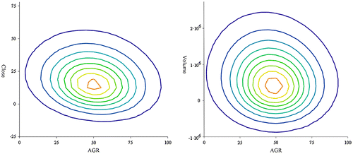
The test sample (companies rating data), following from skew t-distribution, has been simulated by maximum likelihood method and parameters of the skew t-distribution have been estimated using MathCad.

We use the covariance matrix and modelling of correlation in the pricing as a simple proxy for multivariate dependence.

The correlation coefficient is highly informative about the degree of linear dependence, it shows how strongly pairs of variables are related. It ranges from -1.0 to +1.0 (if the correlation is negative, we have a negative relationship; if it is positive, the relationship is positive). The closer correlation coefficient is to +1 or -1, the more closely the two variables are related. If correlation coefficient is close to 0, it means there is no relationship between the variables. Covariance matrices Σ, Θ characterise variance of coordinate variables and their interdependence. In the first case, interdependence is measured between AGR and Volume, and second time between AGR and Close. Standard deviations (Table 3) are estimated from skew t-distribution covariance matrices Σ, Θ. Standard deviation of AGR is a square root of element σ₁₁ from matrix Σ, square root of element σ₂₂ gives standard deviation of Volume. Other standard deviations are obtained from matrix Θ. The same procedure is repeated for AGR and Close prices.

Table 3. Compute skew t-distribution standard deviation of pairs of stocks and AGR.

Period	Matrices	Standard deviation
		AGR	Volume, (×10^6)	AGR	Close
2011_09 (III term)	Sigma	31.749	1.128	36.083	17.797
	Theta	31.890	1.997	30.022	32.249
2011_12 (IV term)	Sigma	31.906	0.522	34.756	18.234
	Theta	31.843	0.976	31.038	32.342
2012_03 (I term)	Sigma	31.318	0.824	34.928	20.536
	Theta	31.392	1.566	30.988	36.551
2012_06 (II term)	Sigma	31.221	0.957	34.409	20.190
	Theta	31.270	1.779	30.903	36.263

We calculated the correlation between Close and forecasted AGR (see Tables 4), by varying prediction horizon (I term – the minimum time lag between the Close and forecasted AGR and the IV-term maximum time lag between the Close and projected AGR). We see that increasing the forecasting horizon did not reveal any correlation trend. The same conclusion can be drawn with the examination of the Volume and the forecast AGR correlation.

Table 4. Compute skew t-distribution correlations of pairs of stocks and AGR.

Period	Matrices	Correlation
		AGR-Volume	AGR-Close
2011_09 (III term)	Sigma	-0.326	-0.133
	Theta	0.111	-0.326
2011_12 (IV term)	Sigma	-0.312	-0.191
	Theta	0.105	-0.218
2012_03 (I term)	Sigma	-0.241	-0.174
	Theta	0.176	-0.233
2012_06 (II term)	Sigma	-0.253	-0.119
	Theta	0.163	-0.176

2.7. Self-organised map

The SOM was taught using unsupervised learning. The training process of SOM did not provide details of the ‘correct’ clusters. The input patterns are presented to the network one by one, in random order. The output nodes compete for each and every pattern. The output node with a reference vector that is closest to the input vector is called the winner. The reference vector of the winner is adjusted in the direction of the input vector, and so are the reference vectors of the surrounding nodes in the output array. The size of adjustment in the reference vectors of the neighbouring nodes is dependent on the distance of that node from the winner in the output array. In this way the output nodes start to represent certain features in the input vectors and nearby nodes form the clusters. We use two learning parameters: the learning rate and the neighbourhood width parameter.

The Kohonen map was considered more or less stable when changing the parameters, the same data vectors were placed close to each other.

3. Self-organised map analysis

SOM input data consists of 198 companies share prices (Close and Volume) stable distribution parameters (alpha, beta, gamma, delta), calculated for each year of the company's history.

Since AGR rating is a measure of corporate integrity based on forensic accounting and corporate governance metrics, and is an indicator of aggressive corporate behaviour which stakeholders can put at risk. It is useful to see how the AGR rating changes are reflected in the share price distribution.

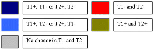
Figure 2 represents the results of the first two maps. It can be seen which neurons includes firms that one period had the AGR upward trend and in the other period had the AGR downward trend. Therefore, in Figures 2 and 3 light blue coloured neurons show which firms got both the AGR upward and downward trend for one period. Red colour coloured neurons shows which firms have the AGR downward trend (a complete explanation is given Figure 3). Green coloured neurons show which companies have the AGR upward trend. The grey coloured neurons denote firms where the AGR rating remains unchanged.

Figure 2. Distribution of companies SOM neurons characterized by AGR upward and downward trends in the period of 2007—2009.

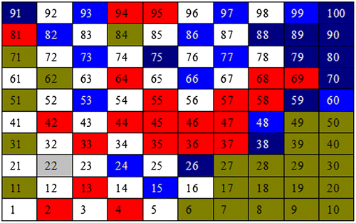
Figure 3. Meaning of different colors in Figure 2. T1+ and T2+ means AGR rating trend towards an increase in the first and second period. T1- and T2- means AGR rating trend to decrease in the first and second period.

So from the Kohonen map we can see the company’s distribution dynamics during the period 2007–2009. Some neurons have stable AGR upward or downward trend. Some neurons are characterised by instability. That is, companies which for one period were characterised by the increase of AGR and the next period by the AGR downward trend. There were also some neurons that had increased or decreased AGR in both periods.

3.1. Random Forests

Random Forests consist of individual decision-tree team. Each decision-tree is trained by using randomly selected data from the training set (two-thirds of all data); the remaining data Out of Bag (OOB) are used for testing. Errors in the test data decrease by increasing the number of decision-trees (Archer & Kimes, 2008; Breiman, 2001; Chan & Paelinckx, 2008; Genuer, Poggi, & Tuleau-Malot, 2010; Hapfelmeier & Ulm, 2013; Liu, Wang, Wang, & Li, 2013).

Feature relevance is measured using the OOB data. Feature selection depends on the amount of data entering the OOB. Therefore, in the selection of key features we started with seven different levels of data. The number of features we denote as N, a number of features falling to the OOB, we will choose as follows:

The features relevance average of OOB was calculated with different amount of data. Using backward elimination of features, we discarded at least 5% of the lowest relevance features, while remained only one feature. We focused on a set of features with the lowest average OOB error (for classification) and with the lowest average relative (relative to the standard deviation of the target) mean squared prediction error (for regression). These features were considered as the most important (Guyon, 2008; Kalsyte, Verikas, Bacauskiene, & Gelzinis, 2013; Verikas, Gelzinis, & Bacauskiene, 2011).

4. Conclusion

The most important features of the indicators used in academic risk models and AGR rating history in predicting future AGR were selected. As the inputs we used indicators of the following academic risk assessment models: the Modified Jones Model, Working Capital Accruals, Beneish M-score and Dechow et al.'s F-score. None of the Working Capital Accruals features were selected as important, and the Beneish's M-score was selected as only one important feature. It was noticed that the important features varies for each AGR class.

The inputs of SOM developed, used AGR history, as well as forecasted future AGR and alpha-stable distribution parameters calculated from the data of stock prices. Stable distribution parameters describe the variation of the shares, while assessing the history of changes in investor sentiment of a specific firm. Meanwhile, the AGR history describes the Audit Integrity Analyst sentiment changes. The Audit Integrity Analyst’s opinion about the company in the future is also predicted. All of that was visualised by SOM. It identifies three clusters, explaining which company’s AGR tends to decrease, increase, and the cluster that reported no clear trend. It also identifies individual neurons, with unstable situations.

Using the skew t-distribution confirms the claim that AGR is related to stock price and volume fluctuations. The results confirmed that the relationship was identified, but is weak.

Disclosure statement

No potential conflict of interest was reported by the authors.

Appendix.

1.	Working Capital Accruals

2.	Beneish’s M-score

Day’s Sales Receivable Index

Gross Margin Index

Asset Equality Index

Sales Growth Index

Depreciation Index

Leverage Index

Sales, General, and Administrative Expenses Index

Total Accruals to Total Assets

3.	Dechow et al.’s F-score

where

Percentage change in cash sales

4.	Modified Jones Model

References

- Archer, K. J., & Kimes, R. V. (2008). Empirical characterization of random forest variable importance measures. Computational Statistics and Data Analysis, 52, 2249–2260.10.1016/j.csda.2007.08.015
- Avramov, D., Chordia, T., Jostova, G., & Philipov, A. (2009). Dispersion in analysts’ earnings forecasts and credit rating. Journal of Financial Economics, 91, 83–101.10.1016/j.jfineco.2008.02.005
- Azzalini, A., & Capitanio, A. (2003). Distributions generated by perturbation of symmetry with emphasis on a multivariate skew t-distribution. Journal of the Royal Statistical Society, Series B: Statistical Methodology, 65, 367–389.10.1111/rssb.2003.65.issue-2
- Azzalini, A., & Genton, M. G. (2008). Robust likelihood methods based on the skew-t and related distributions. International Statistical Review, 76, 106–129.10.1111/j.1751-5823.2007.00016.x
- Breiman, L. (2001). Random forests. Machine Learning, 45, 5–32.10.1023/A:1010933404324
- Cabral, C. R. B., Bolfarine, H., & Pereira, J. R. G. (2008). Bayesian density estimation using skew student-t-normal mixtures. Computational Statistics and Data Analysis, 52, 5075–5090.10.1016/j.csda.2008.05.003
- Chan, J. C. W., & Paelinckx, D. (2008). Evaluation of random forest and adaboost tree-based ensemble classification and spectral band selection for ecotope mapping using airborne hyperspectral imagery. Remote Sensing of Environment, 112, 2999–3011.10.1016/j.rse.2008.02.011
- Enhanced Online News. (2010). Audit integrity’s ‘AGR’ rating outperforms leading academic accounting risk measures, independent study finds. Retrieved from http://eon.businesswire.com/news/eon/20100315006063/en
- Genuer, R., Poggi, J. M., & Tuleau-Malot, C. (2010). Variable selection using random forests. Pattern Recognition Letters, 31, 2225–2236.10.1016/j.patrec.2010.03.014
- Guyon, I. (2008). Practical feature selection: From correlation to causality. In NATO science for peace and security, Vol. 19 of D: Information and communication security, Ch. 3, (pp. 27–43). Amsterdam: IOS Press.
- Hapfelmeier, A., & Ulm, K. (2013). A new variable selection approach using random forests. Computational Statistics and Data Analysis, 60, 50–69.10.1016/j.csda.2012.09.020
- Kabasinskas, A., Rachev, S. T., Sakalauskas, L., Sun, W., & Belovas, I. (2009). α-stable paradigm in financial markets. Journal of Computational Analysis and Applications, 11, 642–688.
- Kabasinskas, A., Rachev, S. T., Sakalauskas, L., Sun, W., & Belovas, I. (2010). Stable mixture model with dependent states for financial return series exhibiting short histories and periods of strong passivity. Journal of Computational Analysis and Applications, 12, 268–292.
- Kalsyte, Z., Verikas, A., Bacauskiene, M., & Gelzinis, A. (2013). A novel technique to design an adaptive committee of models applied to predicting company’s future performance. Expert Systems with Applications: An International Journal archive, 40, 2051–2057.10.1016/j.eswa.2012.10.018
- Kim, H. M., & Mallick, B. K. (2003). Moments of random vectors with skew t distribution and their quadratic forms. Statistics & Probability Letters, 63, 417–423.
- Liu, M., Wang, M., Wang, J., & Li, D. (2013). Comparison of random forest, support vector machine and back propagation neural network for electronic tongue data classification: Application to the recognition of orange beverage and Chinese vinegar. Sensors and Actuators B: Chemical, 177, 970–980.10.1016/j.snb.2012.11.071
- Nikias, C. L., & Shao, M. (1995). Signal processing with alpha-stable distributions and applications. New York, NY: Wiley.
- Nolan, J. P. (2007). Stable distributions – models for heavy tailed data. Boston, MA: Birkhauser.
- Owen, A. (2002). Empirical likelihood. New York, NY: Chapman & Hall.
- Panagiotelis, A., & Smith, M. (2008). Bayesian density forecasting of intraday electricity prices using multivariate skew t distributions. International Journal of Forecasting, 24, 710–727.10.1016/j.ijforecast.2008.08.009
- Price, R. A., Sharp, N. Y., & Wood, D. A. (2011). Detecting and predicting accounting irregularities: A comparison of commercial and academic risk measures. Social Science Research Network. Retrieved from http://ssrn.com/abstract=1546675
- Rachev, S. T., Tokat, Y., & Schwatz, E. S. (2003). The stable Non-Gaussian asset allocation: A comparison with the classical Gaussian approach. Journal of Economic Dynamics & Control, 27, 937–969.
- Ramnath, S., Rock, S., & Shane, P. B. (2008). The financial analyst forecasting literature: A taxonomy with suggestions for further research. International Journal of Forecasting, 24, 34–75.10.1016/j.ijforecast.2007.12.006
- Samorodnitsky, G., & Taqqu, M. S. (2000). Stable Non-Gaussian random processes, stochastic models with infinite variance. New York, NY: Chapman & Hall.
- Spall, J. C. (2003). Introduction to stochastic search and optimization: Estimation, simulation, and control. New York, NY: Wiley.10.1002/0471722138
- Spellman, G. K., & Watson, R. (2009). Corporate governance ratings and corporate performance: An analysis of Governance Metrics International (GMI) ratings of US firms, 2003 to 2008. Social Science Research Network. Retrieved from http://ssrn.com/abstract=1392313
- Verikas, A., Gelzinis, A., & Bacauskiene, M. (2011). Mining data with random forests: A survey and results of new tests. Pattern Recognition, 44, 330–349.10.1016/j.patcog.2010.08.011