Large-scale consensus with endo-confidence under probabilistic linguistic circumstance and its application

Abstract

In real decision-making problems, decision makers (DMs) usually select the most potential project from several ones. However, they unconsciously show different confidence levels in decision-making process because they come from various backgrounds and have different experiences, etc., which affects the decision results. Moreover, the probabilistic linguistic term set, which not only includes the linguistic expressions used by DMs in their daily life but also contains the probability for each linguistic term, can well portray the real perceptions of DMs for the projects. Furthermore, large-scale consensus has gradually been a popular way to effectively solve complex decision-making problems. To sum up, in this paper, we are dedicated to constructing a large-scale consensus model considering the confidence levels of DMs under probabilistic linguistic circumstance. Firstly, the endo-confidence is defined and measured by DM’s probabilistic linguistic information. Then, the DMs are clustered according to the similarities of both evaluation information and the endo-confidence levels. Both evaluation of the non-consensus cluster and evaluation integrated by the clusters with higher endo-confidence level than this non-consensus cluster are used as the reference to adjust its evaluation information. Then, a case study and the comparative analysis are carried out. Finally, some conclusions and future work are given.

Keywords:

• Large-scale consensus
• endo-confidence level
• probabilistic linguistic term set

JEL CODES:

• C10
• C60
• D81

1. Introduction

In our daily life, decision makers (DMs) often evaluate the available projects, which is the main part in the decision-making process. Sometimes, there are many aspects which should be considered due to the complexity of the decision objects (Tian et al., 2021). In order to comprehensively evaluate the projects, DMs need to master different types of knowledge. However, with the development of economy, the social division of labor has been increasingly refined, and the professional knowledge and skills continue to be strengthened. Thus, the single DM can be only specialised in one major and be proficient in a special field. Then, group decision making (GDM) has become a general way to conquer the disadvantages caused by the professionalisation in real decision-making situations.

In GDM process, the DMs come from various professional fields and have different backgrounds. And thus, they may have different opinions for the same project. Sometimes, those opinions may have large difference. If those evaluations with large difference are used to make decisions, the decision results may be unreasonable and distorted. Therefore, reaching consensus is the precondition to make a reasonable decision in GDM. Moreover, for complex decision-making problems, the large number of DMs need to be invited to participate in decision making. Considering the situation above, large-scale consensus has been a hot topic in recent years.

In real decision-making cases, some attributes are not suitable to be expressed as numerical form, and nature languages are the usual form used by DMs in their evaluation processes. In order to deal with natural languages, linguistic expression (Zadeh, 1975) is developed and widely adopted as the basic evaluation information in decision-making methods. As experts may hesitate among several values to assess a project in decision-making process, hesitate fuzzy linguistic term set (HFLTS) has been proposed by Rodriguez et al. (2012) to handle the uncertain environments. However, according to HFLTS, all possible values provided by the DMs have equal importance or weight which may lead to unreasonable decision results (Pang et al., 2016). That is because (1) the occurrence frequencies of evaluation values are likely to be different for a group of DMs, and (2) for a single DM, the reliabilities or the preference degrees on evaluation values are also probably different (Xu, He, et al., 2019). As a result, the probabilistic linguistic term set (PLTS) (Pang et al., 2016), which is a widespread description tool in the existing decision-making method (Wei et al., 2020), can solve the above problem. It not only includes the hesitant linguistic representation but also reflects the different preference degree for each piece of linguistic representation. Hence, in this paper, we will use PLTSs to represent the evaluation information of DMs.

Moreover, DMs are professional individuals in their special fields, and they may have different perceptions for the same aspect of the projects. Then, the confidence levels of their evaluation information are also different. Thus, considering the effect of confidence on the decision-making results is essential. Consensus models with self-confidence have been presented and Ding et al. (2019) alleged that the self-confidence level indeed affect the consensus reaching process. According to Liu et al. (2017) and Liu et al. (2018) proposed an iteration-based consensus with self-confidence multiplicative preference relations. Gou, Xu, Wang, et al. (2021) introduced self-confidence factor into the double hierarchy linguistic preference relations and presented a consensus model based on the priority ordering theory. Zhang et al. (Zhang et al., 2021) introduced self-confidence factor into comparative linguistic expressions and gave an optimisation consensus model with minimum information loss. Liu, Xu, Montes, and Herrera (2019) focussed on the self-confidence-based consensus model and proposed a novel feedback mechanism that chooses the expert with minimal self-confidence to adjust his/her evaluation information.

Consistency of preference relation in consensus model should also be considered (Gou et al., 2019). It is easy to notice that some researches based on preference relations with self-confidence neglect the consistency of the preference relations, which has a direct influence on the results of final decision (Liu, Xu, Montes, Dong, et al., 2019). To solve this problem, Liu, Xu, Montes, Dong, et al. (2019) gave a novel method to measure the additive consistency level by considering both the fuzzy preference values and the self-confidence levels. However, additive consistency sometimes cannot capture the consistency of a fuzzy preference relation (Zhang, Kou, et al., 2020). Zhang, Kou, et al. (2020) proposed two algorithms to improve the multiplicative consistency level. Bashir et al. (2018) defined the hesitant fuzzy preference relation with self-confidence and the hesitant multiplicative preference relation with self-confidence in their paper, and also the corresponding additive consistency and multiplicative consistency.

As the development of technology, large-scale decision making has been more and more popular. Based on Xu, Du, et al. (2019), the combination of the levels of both rationality and non-cooperation is used to measure the confidence level, which is utilised as adjustment coefficient to modify the evaluation value. According to Liu et al. (2017), Liu, Xu, and Herrera (2019) studied the large-scale consensus which considers the overconfidence behaviours of DMs. The grey clustering algorithm was used to distinguish the experts by combining the similarities of both fuzzy preference values and self-confidence levels. An overconfidence measurement was given to detect the experts’ overconfidence behaviours in the consensus model. Also, a dynamic weight punishment mechanism was implemented to manage overconfidence behaviour. However, the clustering method in Liu, Xu, and Herrera (2019) causes the problem that the experts with lower similarities of fuzzy preference values will be classified into one cluster because they have the higher similarities of self-confidence levels. Then, these experts with large differences in fuzzy preference will be used to calculate the weights together and further to obtain the overall preference value, which may lead to unreasonable decision-making results.

As far as we know, in the existing literature, self-confidence level is directly given by DMs and there are not any consensus researches considering to measure the confidence from the evaluation information. Because there are not any consensus researches considering the confidence of DMs with PLTS, our research targeted at consensus with PLTS for multi-attribute large-scale GDM (LSGDM) problems typically has four main goals:

1. In order to give the DMs’ confidence level more accurately and objectively, and distinguish the self-confidence given by DM in the existing studies, one aim is to define the endo-confidence, which is measured by DM’s evaluation information rather than the existing self-confidence given by the DM aforehand.

2. To solve the problem of confidence-based clustering that DMs with lower similarities of evaluations may be classified into one cluster, one purpose is to define a novel clustering procedure based on both the evaluation information and the endo-confidence level.

3. In the decision-making process, the DMs with higher level of endo-confidence may influence the opinions of others whose confidence levels are lower than themselves. Also, those DMs with higher endo-confidences tend to have a greater impact on the final results than those DMs with lower endo-confidences. Hence, one objective is to simulate the above phenomenon and present a new feedback adjustment mechanism.

4. When assigning the missing probabilities to linguistic terms for the incomplete PLTSs, the total probability for linguistic terms from DMs should be considered. Moreover, the original preference among linguistic terms of DMs should also be considered when normalising the PLTSs. In order to reflect the opinions of DMs more accurately and avoid the loss of information, the other goal is to provide a suitable method to normalise the PLTSs.

To sum up, in this paper, we will construct the large-scale consensus model with probabilistic linguistic information considering the confidence behaviours (which is named as endo-confidence level in this paper) of DMs derived from PLTS itself. Although there already exists large-scale consensus models considering the self-confidence behaviours, it is different according to our above review. The innovations of this paper can be summarised as follows:

1. In this paper, the endo-confidence is defined and it can be obtained from three aspects: (a) the probabilistic information in the original evaluation given by DMs; (b) DMs’ hesitation in the original evaluation information; and (c) DMs’ preference among linguistic terms in the original evaluation information.

2. Inspire by the similarity-based clustering algorithm, we give a new bi-clustering process considering both the evaluation information and the endo-confidence level. The optimal classification threshold is determined by both the similarities and the threshold given by DMs.

3. We consider the evaluation information of both the cluster itself and the clusters with higher endo-confidence levels than itself as the reference to adjust the evaluation information of this cluster. Meanwhile, an endo-confidence-based method to determine weights is proposed. In this method, we give a function to obtain the weights.

4. We proposed a new method to normalise the PLTSs, which considers both the certainty degree of probabilistic information and the preference among the linguistic terms in it.

The outline of this paper is listed as follows: Section 2 shows the preliminaries including the form of basic evaluation information and its operators. Consensus reaching process is given in Section 3, including how to determine the endo-confidence level, how to normalise the PLTSs and the weights of DMs, clustering process, consensus measurement, feedback mechanism and the selection process. Then, a case study and comparative analysis are shown in Section 4. Finally, Section 5 ends with some conclusions.

2. Preliminaries

In this section, we will introduce the basic knowledge proposed in previous studies, such as the linguistic term set, the probabilistic linguistic term set and its score function, distance and similarity measurements, etc., which will be used in this paper.

2.1. The probabilistic linguistic term set

Linguistic is generally used in our daily life to express DMs’ opinions. The linguistic variable (Zadeh, 1975) is closer to the natural or artificial language and has been widely used in the decision-making field. Let $S=\{s_0,s_1,\dots ,s_{\gamma },\dots ,s_{\tau }\}$ be a linguistic term set (LTS), where $s_{\gamma }$ represents the $\gamma$-th linguistic term in $S,$ and $\tau +1$ is the cardinality of the LTS $S.$

Then, the PLTS (Pang et al., 2016) with probability of each linguistic term is defined as: (1) $$L(p)=\{L^{(k)}(p^{(k)})|L^{(k)}\in S,p^{(k)}\ge 0,k=1,2,\dots ,\#L(p),\sum _{k=1}^{\#L(p)}{p}^{(k)}\le 1\}$$(1) where $L^{(k)}(p^{(k)})$ is a linguistic term $L^{(k)}$ associated with the probability $p^{(k)},$ and $\#L(p)$ is the number of all different linguistic terms in $L(p).$ When ${\sum }_{k=1}^{\#L(p)}{p}^{(k)}<1,$ we should normalise it to be ${\sum }_{k=1}^{\#L(p)}{p}^{(k)}=1$ before the aggregation processes. In this paper, we will give a new normalised method in Section 3.2.

In order to reflect the assessments of experts with PLTSs and make a comparison among different PLTSs, Pang et al. (2016) defined the score function $E(L(p))$ of $L(p)$ as: (2) $$E(L(p))=s_{\overline{\upsilon }}$$(2) where $\overline{\upsilon }={\sum }_{k=1}^{\#L(p)}{\gamma }^{(k)}{p}^{(k)}/{\sum }_{k=1}^{\#L(p)}{p}^{(k)},$ and ${\gamma }^{(k)}$ means the subscript of linguistic term $L^{(k)}.$ If $s_{\overline{\upsilon }}\notin S,$ it is named as virtual linguistic term (Xu, 2004). For two PLTSs $L^1(p)$ and $L^2(p),$ if $\overline{{\upsilon }^1}>\overline{{\upsilon }^2},$ then $L^1(p)$ is superior to $L^2(p),$ denoted by $L^1(p)\succ L^2(p);$ if $\overline{{\upsilon }^1}<\overline{{\upsilon }^2},$ then $L^1(p)$ is inferior to $L^2(p),$ denoted by $L^1(p)\prec L^2(p);$ if $\overline{{\upsilon }^1}=\overline{{\upsilon }^2},$ then there is $L^1(p)\sim L^2(p).$

2.2. The distance and the similarity between PLTSs

Distance is a general tool used to reflect the relationship of PLTSs. Pang et al. (2016) and Zhang et al. (2016) defined two methods to obtain the distance among PLTSs. However, both of those two methods need to add linguistic terms to a shorter PLTS, which may lead to biased results (Wu et al., 2018). To solve this problem, Wu et al. (2018) introduced a novel method to adjust the linguistic terms with different probability distributions into those with the same probability distribution. The method effectively avoids the problem of information loss by the unchanged linguistic terms and the sum of their probabilities. Hence, this method (Wu et al., 2018) is used in this paper to make two PLTSs have the same length, so that we can measure the distance between them. Here, we give a brief description of this method.

Let $\overline{L^1(p)}=\{\overline{L^{1(k)}}(\overline{p^{1(k)}})|k=1,2,\dots ,\#\overline{L^1(p)}\}$ and $\overline{L^2(p)}=\{\overline{L^{2(k)}}(\overline{p^{2(k)}})|k=1,2,\dots ,\#\overline{L^2(p)}\}$ be two normalised PLTSs and the subscripts of the linguistic terms in them are ranked as ascending/descending order. Suppose that the rearranged probabilistic distributions of $\overline{L^1(p)}$ and $\overline{L^2(p)}$ are the same as ${\overline{p}}^{\ast }=\left\{{\overline{p^{(k^{\prime })}}}^{\ast }\right|k^{\prime }=1,2,\dots ,\#{\overline{L^{1,2}(p)}}^{\ast }\}.$ Then, we can obtain the rearranged PLTSs of $\overline{L^1(p)}$ and $\overline{L^2(p)},$ denoted as ${\overline{L^1(p)}}^{\ast }=\{\overline{L^{1(k^{\prime })}}({\overline{p^{(k^{\prime })}}}^{\ast })|k^{\prime }=1,2,\dots ,\#{\overline{L^1(p)}}^{\ast }\}$ and ${\overline{L^2(p)}}^{\ast }=\{\overline{L^{2(k^{\prime })}}({\overline{p^{(k^{\prime })}}}^{\ast })|k^{\prime }=$ $1,2,\dots ,\#{\overline{L^2(p)}}^{\ast }\}$ by the following steps:

Step 1. Let ${\overline{p^{(1)}}}^{*}=\min \{\overline{p^{1(1)}},\overline{p^{2(1)}}\}.$

Step 2. Then we can calculate ${\overline{p^{(2)}}}^{\ast }.$

1. If ${\overline{p^{(1)}}}^{\ast }=\overline{p^{1(1)}},$ then ${\overline{p^{(2)}}}^{\ast }=\min \{\overline{p^{1(2)}},\overline{p^{2(1)}}-{\overline{p^{(1)}}}^{\ast }\}.$

2. If ${\overline{p^{(1)}}}^{\ast }=\overline{p^{2(1)}},$ then ${\overline{p^{(2)}}}^{\ast }=\min \{\overline{p^{2(2)}},\overline{p^{1(1)}}-{\overline{p^{(1)}}}^{\ast }\}.$

Step 3. Obtain ${\overline{p^{(3)}}}^{\ast }$ by using the following rules:

1. If ${\overline{p^{(1)}}}^{\ast }=\overline{p^{1(1)}}$ and ${\overline{p^{(2)}}}^{\ast }=\overline{p^{1(2)}},$ then ${\overline{p^{(3)}}}^{\ast }=\min \{\overline{p^{1(3)}},\overline{p^{2(1)}}-{\overline{p^{(1)}}}^{\ast }-{\overline{p^{(2)}}}^{\ast }\}.$

2. If ${\overline{p^{(1)}}}^{\ast }=\overline{p^{1(1)}}$ and ${\overline{p^{(2)}}}^{\ast }=\overline{p^{2(1)}}-{\overline{p^{(1)}}}^{\ast },$ then ${\overline{p^{(3)}}}^{\ast }=\min \{\overline{p^{1(2)}}-{\overline{p^{(2)}}}^{\ast },\overline{p^{2(2)}}\}.$

3. If ${\overline{p^{(1)}}}^{\ast }=\overline{p^{2(1)}}$ and ${\overline{p^{(2)}}}^{\ast }=\overline{p^{2(2)}},$ then ${\overline{p^{(3)}}}^{\ast }=\min \{\overline{p^{2(3)}},\overline{p^{1(1)}}-{\overline{p^{(1)}}}^{\ast }-{\overline{p^{(2)}}}^{\ast }\}.$

4. If ${\overline{p^{(1)}}}^{\ast }=\overline{p^{2(1)}}$ and ${\overline{p^{(2)}}}^{\ast }=\overline{p^{1(1)}}-{\overline{p^{(1)}}}^{\ast },$then ${\overline{p^{(3)}}}^{\ast }=\min \{\overline{p^{2(2)}}-{\overline{p^{(2)}}}^{\ast },\overline{p^{1(2)}}\}$

Step 4. We can calculate other rearranged probability distributions by the above rules.

Notes:

1. We can find that ${\overline{p^{(\#{\overline{L^{1,2}(p)}}^{\ast })}}}^{\ast }=\min \{\overline{p^{1(\#\overline{L^1(p)})}},\overline{p^{2(\#\overline{L^2(p)})}}\}$.

2. The length of the rearranged PLTSs is equal, that is $\#{\overline{L^1(p)}}^{\ast }=\#{\overline{L^2(p)}}^{\ast }=\#{\overline{L^{1,2}(p)}}^{\ast }.$

3. It should be satisfied that $\overline{p^{1(k)}}={\overline{p^{(k^{\prime })}}}^{\ast }+{\overline{p^{(k^{\prime }+1)}}}^{\ast }+\cdots +{\overline{p^{(k^{\prime }+{\iota }_1)}}}^{\ast },$ where $\overline{p^{1(k)}}$ is the probability of $\overline{L^{1(k)}}$ in $\overline{L^1(p)},$ ${\overline{p^{(k^{\prime })}}}^{\ast },{\overline{p^{(k^{\prime }+1)}}}^{\ast },\dots ,{\overline{p^{(k^{\prime }+{\iota }_1)}}}^{\ast }$ are the probabilities of $\overline{L^{1(k^{\prime })}}$ in ${\overline{L^1(p)}}^{\ast },$ and the subscript of the rearranged terms $\overline{L^{1(k^{\prime })}},\overline{L^{1(k^{\prime }+1)}},\dots ,\overline{L^{1(k^{\prime }+{\iota }_1)}}$ is equal to the subscript of the original normalised terms $\overline{L^{1(k)}}.$ The linguistic terms in $\overline{L^2(p)}$ satisfy this condition, too. In other words, the linguistic terms and the sum of their probabilities are not changed in the rearranged PLTSs.

4. The subscripts of the linguistic terms in the rearranged PLTSs are ranked as non-ascending/non-descending order.

In order to use data more efficiently and express the semantics flexibly, Wang et al. (2014) proposed the linguistic scale function $f$ which is a monotonically increasing function, where $f:s_{\gamma }\to {\theta }_{\gamma };$ $f^{-1}:{\theta }_{\gamma }\to s_{\gamma };$ ${\theta }_{\gamma }\in [0,1].$ Then, it is represented by: (3) $$f(s_{\gamma })=\frac{\gamma }{\tau },f^{-1}({\theta }_{\gamma })=s_{\tau \cdot {\theta }_{\gamma }}$$(3)

Wu and Liao (2019) introduced the linguistic scale to measure the distance by Equation (4)(4) $$d(\overline{L^1(p)},\overline{L^2(p)})=\sum _{k^{\prime }=1}^{\#{\overline{L^{1,2}(p)}}^{\ast }}{\overline{p^{(k^{\prime })}}}^{\ast }|f(\overline{L^{1(k^{\prime })}})-f(\overline{L^{2(k^{\prime })}})|$$(4) : (4) $$d(\overline{L^1(p)},\overline{L^2(p)})=\sum _{k^{\prime }=1}^{\#{\overline{L^{1,2}(p)}}^{\ast }}{\overline{p^{(k^{\prime })}}}^{\ast }|f(\overline{L^{1(k^{\prime })}})-f(\overline{L^{2(k^{\prime })}})|$$(4)

According to Wu et al. (2018), we can obtain the similarity of the PLTSs $\rho (\overline{L^1(p)},\overline{L^2(p)})$ based on their distance $d(\overline{L^1(p)},\overline{L^2(p)}):$ (5) $$\rho (\overline{L^1(p)},\overline{L^2(p)})=1-d(\overline{L^1(p)},\overline{L^2(p)})$$(5)

3. Consensus decision making with endo-confidence based on the probabilistic linguistic information

In this section, we will give a new procedure to reach consensus considering the endo-confidence levels of DMs. Firstly, we will show how to determine the endo-confidence level of each DM from his/her evaluation information. Then, a new method to normalise the PLTSs is given. After that, a similarity-based clustering algorithm is used to distinguish the DMs into several clusters with bi-clustering. The weight of each DM is an important issue in decision making, and we will define a method to measure the weight of DM based on his/her endo-confidence level. Subsequently, a consensus measurement is carried out and the identification and adjustment procedures are designed to achieve consensus. Finally, when the consensus level is reached, the selection process is presented. Please see Table A1 for the meaning of notations used in the proposed model.

3.1. How to determine the endo-confidence level of each DM

As afore-mentioned, the experts’ confidence levels greatly influence the final decision-making results and it should be considered in the decision-making process. As a key step, the measurement of confidence level should be further discussed. However, few studies measure the confidence level according to the evaluation information (Guha & Chakraborty, 2011), especially through probabilistic linguistic information. As a result, in this paper, we propose a method to determine experts’ original confidence levels which are named endo-confidence levels based on probabilistic linguistic information from those three aspects:

• (1) The probabilistic information in the original evaluation given by experts

The original probabilities given by experts can reflect their endo-confidence levels. It is not difficult to find that the greater the total probability of the original assessment from an expert is, the higher the expert’s endo-confidence level for the corresponding assessment. For instance, if an expert ($e^1$) gives his/her assessment as $L^1(p)=\{s_3(0.2),s_4(0.1)\}$ while another expert ($e^2$) gives his/her assessment as $L^2(p)=\{s_3(0.6),s_4(0.3)\},$ we can find that the expert $e^2$ gives more information than the expert $e^1.$ That is, the expert $e^2$ is more confident for his/her evaluation information than the expert $e^1.$ Hence, we can calculate endo-confidence level from the perspective of total probability by $e{c}_p={\sum }_{k=1}^{\#L(p)}{p}^{(k)}.$ The first part of endo-confidence level of expert $e^1$/$e^2$ is denoted as $e{c}_p^1=0.3$/$e{c}_p^2=0.9.$

• (2) Experts’ hesitation in the original evaluation information

Experts may express various degrees of hesitation when facing a decision-making problem. The greater degree of hesitation means that the experts are less confident. Furthermore, endo-confidence level should be related to the number of the linguistic terms in PLTS. For instance, if there are two PLTSs $L^1(p)=\{s_0(0.1),s_1(0.2),s_2(0.3),s_3(0.2),s_4(0.1)\}$ and $L^2(p)=\{s_3(0.6),s_4(0.3)\}$ given by experts $e^1$ and $e^2$ respectively. Intuitively, the expert $e^1$ is more hesitant than the expert $e^2.$ That is, $e^1$ is less confident about his/her evaluation information than $e^2.$ Hence, the endo-confidence level based on hesitation is defined as: $e{c}_h=1-\frac{\#L(p)-1}{\tau }.$

• 1. When $\frac{\#L(p)-1}{\tau }=0,$ it means that the expert gives only one linguistic term. Under this circumstance, expert does not hesitate about his/her evaluation, and there is $e{c}_h=1.$

• 2. When $\frac{\#L(p)-1}{\tau }=1,$ it means $\#L(p)=\tau +1,$ and the expert believes that all linguistic terms in $S$ may be the possible evaluation, and thus, there is $e{c}_h=0.$

• 3. In other cases, the value of endo-confidence level of the expert is somewhere between the above two cases, that is, $0<e{c}_h<1.$

• (3) Experts’ preference among linguistic terms in the original evaluation information

One of the most important characteristics of probabilistic linguistic information is that it can reflect the preferences of DMs among the linguistic terms in PLTSs. We can get another part of the expert’s endo-confidence level from the probability distribution in different linguistic terms.

Example 1.

If the experts $e^1,$ $e^2$ and $e^3$ give their assessments as $L^1(p)=\{s_2(0.1),s_3(0.2)\},$ $L^2(p)=$ $\{s_2(0.3),s_3(0.6)\}$ and $L^3(p)=\{s_2(0.4),s_3(0.4)\}$ respectively, we can find that the expert $e^3$ does not know which of the linguistic terms $s_2$ and $s_3$ is better, while the expert $e^2$ thinks that the linguistic term $s_3$ can better describe his/her perception than $s_2.$ Motivated by the concept of standard deviation in depicting the degree of dispersion, we can find that a smaller standard deviation level of probabilities means that the probabilities are closer, and endo-confidence level of the expert is lower, while a larger standard deviation indicates that the expert has a stronger preference for some linguistic terms, which shows that the expert is more confident. Hence, the standard deviation of probabilities should be used as a measure of endo-confidence level. It is worth noting that the expert $e^1$ and the expert $e^2$ have the same preference for the terms $s_2$ and $s_3,$ but the standard deviation levels of probabilities are different due to the difference in total probabilities. The standard deviation of the probabilities in $L^1(p)$ is 0.05, while the standard deviation of the probabilities in $L^2(p)$ is 0.15.

In order to solve this problem, inspired by Pang et al. (2016), we first adjust the total probability to 1 according to the given information. In particular, the associated PLTS $L(p{)}^{\prime }$ is defined by $L^{\prime }(p)=\{L^{(k)}({p^{\prime }}^{(k)})|k=1,2,\dots ,\#L^{\prime }(p)\},$ where ${p^{\prime }}^{(k)}=p^{(k)}/{\sum }_{k=1}^{\#L(p)}{p}^{(k)}.$ We can further calculate standard deviation level $\mathit{std}$ of probabilities ${p^{\prime }}^{(k)}:$ (6) $$\mathit{std}=\sqrt{\frac{\sum _{k=1}^{\#L^{\prime }(p)}{[{p^{\prime }}^{(k)}-\frac{1}{\#L^{\prime }(p)}\sum _{k=1}^{\#L^{\prime }(p)}{p^{\prime }}^{(k)}]}^2}{\#L^{\prime }(p)}}$$(6) and $\#L^{\prime }(p)$ is the number of all different linguistic terms in $L^{\prime }(p).$

Specially, for the PLTS with only one term, we add a term to it and define the corresponding probability as zero. Then, the standard deviation of probabilities is 0.5.

Then, if there is a finite set of experts $E=\{e^1,e^2,\dots ,e^t\}$ ($T=\{1,2,\dots ,t\},$ $a\in T,$ $t\ge 20$) and the evaluation information of an expert $e^a$ is shown as PLTS, the endo-confidence level $e{c}_d^a$ of $e^a$ from the perspective of preference among linguistic terms can be obtained by Equation (7)(7) $$e{c}_d^a=\frac{st{d}^a-\min \{st{d}^t,\forall t\in T\}}{\max \{st{d}^t,\forall t\in T\}-\min \{st{d}^t,\forall t\in T\}}$$(7) : (7) $$e{c}_d^a=\frac{st{d}^a-\min \{st{d}^t,\forall t\in T\}}{\max \{st{d}^t,\forall t\in T\}-\min \{st{d}^t,\forall t\in T\}}$$(7) where $\min \{st{d}^t,\forall t\in T\}$ means that the minimum standard deviation level of probabilities given by all the experts and $\max \{st{d}^t,\forall t\in T\}$ denotes the corresponding maximum one.

Example 2.

According to Example 1, there is ${L^{\prime }}^1(p)=\{s_2(0.33),s_3(0.67)\},$ ${L^{\prime }}^2(p)=\{s_2(0.33),s_3(0.67)\}$ and ${L^{\prime }}^3(p)=\{s_2(0.5),s_3(0.5)\}$ for the experts $e^1,$ $e^2$ and $e^3$ respectively. Then, we utilise Equation (6)(6) $$\mathit{std}=\sqrt{\frac{\sum _{k=1}^{\#L^{\prime }(p)}{[{p^{\prime }}^{(k)}-\frac{1}{\#L^{\prime }(p)}\sum _{k=1}^{\#L^{\prime }(p)}{p^{\prime }}^{(k)}]}^2}{\#L^{\prime }(p)}}$$(6) to calculate the standard deviation level $\mathit{std},$ $st{d}^1=st{d}^2=0.17,$ and $st{d}^3=0.$ Finally, we get the endo-confidence level $e{c}_d^1=e{c}_d^2=1$ and $e{c}_d^3=0.$

After giving the calculation methods of $e{c}_p,$ $e{c}_h$ and $e{c}_d,$ we can obtain the endo-confidence level $e{c}^a$ of the expert $e^a$ as: (8) $$e{c}^a=\alpha \cdot e{c}_p^a+\beta \cdot e{c}_h^a+(1-\alpha -\beta )\cdot e{c}_d^a$$(8)

$\alpha$ and $\beta$ are two parameters determined by the DM.

Let $A=\{A_1,A_2,\dots ,A_n\}$ ($N=\{1,2,\dots ,n\},$ $i\in N,$ $n\ge 3$) be a finite set of potential alternatives and $C=\{c_1,c_2,\dots ,c_m\}$ ($M=\{1,2,\dots ,m\},$ $j\in M,$ $m\ge 2$) be a finite set of attributes. Suppose that the decision-making matrix from the expert $e^a$ is given as: (9) $$\begin{array}{c}{c}_1{c}_2\cdots c_m\\ X^a=\begin{array}{c}{A}_1\\ A_2\\ ⋮\\ A_n\end{array}{\left[\begin{array}{cccc}{x}_{11}^a& x_{12}^a& \cdots & x_{1m}^a\\ x_{21}^a& x_{22}^a& \cdots & x_{2m}^a\\ ⋮& ⋮& x_{ij}^a& ⋮\\ x_{n1}^a& x_{n2}^a& \cdots & x_{nm}^a\end{array}\right]}_{n\times m},a\in T\end{array}$$(9) where $x_{ij}^a$ ($i\in N,$ $j\in M,$ $a\in T$) is represented by the PLTS $L_{ij}^a(p_{ij}^a)$ which is a piece of probabilistic linguistic information for the alternative $A_i$ on the attribute $c_j$ given by the expert $e^a.$ Then, we can get the endo-confidence matrix of the expert $e^a$ as: (10) $$\begin{array}{c}{c}_1{c}_2\cdots c_m\\ E{C}^a=\begin{array}{c}{A}_1\\ A_2\\ ⋮\\ A_n\end{array}{\left[\begin{array}{cccc}e{c}_{11}^a& e{c}_{12}^a& \cdots & e{c}_{1m}^a\\ e{c}_{21}^a& e{c}_{22}^a& \cdots & e{c}_{2m}^a\\ ⋮& ⋮& e{c}_{ij}^a& ⋮\\ e{c}_{n1}^a& e{c}_{n2}^a& \cdots & e{c}_{nm}^a\end{array}\right]}_{n\times m},a\in T\end{array}$$(10) where $e{c}_{ij}^a$ can be calculated by Equation (8)(8) $$e{c}^a=\alpha \cdot e{c}_p^a+\beta \cdot e{c}_h^a+(1-\alpha -\beta )\cdot e{c}_d^a$$(8) .

3.2. How to normalise the PLTSs

Many scholars have proposed some methods to execute the normalisation of PLTSs. Mi et al. (2020) divided these methods into five categories according to different methods of assigning unknown information, that is, (1) average assignment, (2) full-set assignment, (3) pow-set assignment, (4) envelope assignment, and (5) attitude-based assignment. Furthermore, Zhang, Liao, et al. (2020) gave a new method to normalise the incomplete PLTS into the complete one by assigning the unknown probabilities evenly to all the linguistic terms in $S.$

Although previous researches have given various methods to assign the ignorance of probabilistic information, there are some unreasonable points in these methods. For example, the average assignment method assumes that if a linguistic term $s_{\gamma }$ does not appear in $L(p),$ then it should not appear in the normalised PLTS $\overline{L(p)}.$ However, experts cannot accurately know the linguistic terms associated with the ignorance of probabilistic information. As a result, this assumption imposes too many restrictions on the ignorance of probabilistic information. The full-set assignment method (Fang et al., 2020) and the method proposed by Zhang, Liao, et al. (2020) assign the unknown probabilities to all the linguistic terms which can avoid the problem of too strict restrictions mentioned above. For $\{s_4(0.4),s{}_5(0.5)\},$ if we use average assignment method, there is $\{s_4(0.44),s{}_5(0.56)\},$ while if we use full-set assignment method, there is $\{s_4(0.4),s{}_5(0.5),\{s_0,s_1,s_2,s_3,s_4,s_5,s_6\}(0.1)\},$ and if we use the method proposed by Zhang, Liao, et al. (2020), there is $\{s_0(0.014),s_1(0.014),s_2(0.014),s_3(0.014),s_4(0.415),$ $s{}_5(0.515),s_6(0.014)\}.$ Compared with the average assignment method, the latter two methods assign the unknown information to more terms of the PLTSs. However, those methods do not consider the attitude of DMs. Although the attitudes of DMs (such as optimistic, pessimistic and neutral) are considered in the attitude-based assignment method (Song & Li, 2019), it is not easy to judge the attitudes of DMs in real decision-making process. As a result, inspired by the score function $E(L(p))$ of $L(p),$ we propose a novel method to normalise the incomplete PLTSs.

Since the limitation of knowledge and ability, some DMs will give less assessment which lead to the ignorance of probabilistic information in the decision-making process. It is clear that the more unknown assessment is, the less accurate the information provided by DMs will be. For instance, there are two PLTSs $L^1(p)=\{s_4(0.4),s_5(0.5)\}$ and $L^2(p)=\{s_4(0.1),s_5(0.2)\}.$ Both of the experts deem that the assessment should be between $s_4$ and $s_5,$ but the corresponding probabilities show that the certainty of the assessment $L^1(p)$ reaches 0.9, while the certainty of $L^2(p)$ is only 0.3. It is clear that different normalisation methods should be adopted according to the ignorance of probabilistic information. If the total probability of the PLTS is at a higher level, we tend to believe that experts are more certain about their assessments, thus the remaining probabilities are also distributed around the original information. If the total probability of the PLTS is at a lower level, the assessments may not be accurate. In other words, the remaining probabilities should be assigned to more linguistic terms which are far from the original linguistic information. Hence, we use the values of the ignorance of probabilities to determine the terms that appear in the normalised PLTSs. The specific method is shown as follows:

We can calculate the lower and upper bounds of the normalised PLTS, which is denoted as $s_l$ and $s_u$ respectively, where $l$ and $u$ are obtained by Equations (11)(11) $$l=\max [-\frac{1}{2}\cdot (1-{\sum }_{k=1}^{\#L(p)}{p}^{(k)})\cdot (\tau +1)+\underset{k}{\min }{\gamma }^{(k)},0]$$(11) and (12)(12) $$u=\min [\frac{1}{2}\cdot (1-{\sum }_{k=1}^{\#L(p)}{p}^{(k)})\cdot (\tau +1)+\underset{k}{\max }{\gamma }^{(k)},\tau ]$$(12) : (11) $$l=\max [-\frac{1}{2}\cdot (1-{\sum }_{k=1}^{\#L(p)}{p}^{(k)})\cdot (\tau +1)+\underset{k}{\min }{\gamma }^{(k)},0]$$(11) (12) $$u=\min [\frac{1}{2}\cdot (1-{\sum }_{k=1}^{\#L(p)}{p}^{(k)})\cdot (\tau +1)+\underset{k}{\max }{\gamma }^{(k)},\tau ]$$(12)

Notice that:

1. When $1-{\sum }_{k=1}^{\#L(p)}{p}^{(k)}=0,$ the PLTS is a complete one. In this case, $l=\underset{k}{\min }{\gamma }^{(k)}$ and $u=\underset{k}{\max }{\gamma }^{(k)},$ the lower and upper bounds of the normalised PLTS are the same as the original one.

2. When $1-{\sum }_{k=1}^{\#L(p)}{p}^{(k)}=1,$ all of the assessments are unknown, and thus, the normalised LTS should fetch all the linguistic terms, in other words, $s_l=s_0$ and $s_u=s_{\tau }.$ In this condition, we can give a virtual PLTS as $\{s_{\frac{\tau }{2}}(0)\}$ and utilise Equations (11)(11) $$l=\max [-\frac{1}{2}\cdot (1-{\sum }_{k=1}^{\#L(p)}{p}^{(k)})\cdot (\tau +1)+\underset{k}{\min }{\gamma }^{(k)},0]$$(11) and (12)(12) $$u=\min [\frac{1}{2}\cdot (1-{\sum }_{k=1}^{\#L(p)}{p}^{(k)})\cdot (\tau +1)+\underset{k}{\max }{\gamma }^{(k)},\tau ]$$(12) to get its corresponding lower and upper bounds.

3. Specifically, if the bounds of the normalised PLTS exceed the definition of the LTS, then we set $s_l=s_0$ and $s_u=s_{\tau }.$

Subsequently, we fill in all integer terms between $s_l$ and $s_u$ to get the normalised LTS $\overline{L}=\{s_l,\dots ,s_{\gamma },\dots ,s_u\}.$ Then, we get the corresponding expanded original probabilities $p_{\varsigma }^{(k^{\prime })}$ according to Equation (13)(13) $$p_{\varsigma }^{(k^{\prime })}=\{\begin{array}{c}{p}^{(k)}\exists \overline{L^{(k^{\prime })}}=L^{(k)}\\ 0\mathit{otherwise}\end{array}$$(13) and obtain the PLTS $\overline{L(p_{\varsigma })}=\{\overline{L^{(k^{\prime })}}(p_{\varsigma }^{(k^{\prime })})|p_{\varsigma }^{(k^{\prime })}\ge 0,k^{\prime }=1,2,\dots ,\#\overline{L(p_{\varsigma })},{\sum }_{k^{\prime }=1}^{\#\overline{L(p_{\varsigma })}}{p}_{\varsigma }^{(k^{\prime })}\le 1\}:$ (13) $$p_{\varsigma }^{(k^{\prime })}=\{\begin{array}{c}{p}^{(k)}\exists \overline{L^{(k^{\prime })}}=L^{(k)}\\ 0\mathit{otherwise}\end{array}$$(13) where $\#\overline{L(p_{\varsigma })}$ is the number of all different linguistic terms in $\overline{L(p_{\varsigma })}.$

When normalising the probabilistic linguistic information, we should consider the original opinions of experts. The term which is closer to the score $E(L(p))$ is more in line with the original opinion of the expert, and we should assign a greater probability to this term. When ${\gamma }^{(k^{\prime })}=\overline{\upsilon }$ (see Equation (2)(2) $$E(L(p))=s_{\overline{\upsilon }}$$(2) ), the proportion of the probability distribution $h(p^{(k^{\prime })})$ should be maximised. In this paper, we use the exponential function to obtain $h(p^{(k^{\prime })}):$ (14) $$h(p^{(k^{\prime })})=\{\begin{array}{c}\hspace{0.17em}\text{exp}\hspace{0.17em}({\gamma }^{(k^{\prime })})ifl\le {\gamma }^{(k^{\prime })}\le \overline{\upsilon }\\ \hspace{0.17em}\text{exp}[2\cdot \overline{\upsilon }-{\gamma }^{(k^{\prime })}]if\overline{\upsilon }<{\gamma }^{(k^{\prime })}\le u\end{array}$$(14)

Equation (15)(15) $$\overline{h(p^{(k^{\prime })})}=\frac{h(p^{(k^{\prime })})}{\sum _{k^{\prime }=1}^{\#\overline{L(p_{\varsigma })}}h(p^{(k^{\prime })})}$$(15) is used to get the normalised proportion $\overline{h(p^{(k^{\prime })})}$ of the probability distribution: (15) $$\overline{h(p^{(k^{\prime })})}=\frac{h(p^{(k^{\prime })})}{\sum _{k^{\prime }=1}^{\#\overline{L(p_{\varsigma })}}h(p^{(k^{\prime })})}$$(15)

Then, we can obtain the normalised probabilities $\overline{p^{(k^{\prime })}}:$ (16) $$\overline{p^{(k^{\prime })}}=\overline{h(p^{(k^{\prime })})}\cdot (1-{\sum }_{k^{\prime }=1}^{\#\overline{L(p_{\varsigma })}}{p}_{\varsigma }^{(k^{\prime })})+p_{\varsigma }^{(k^{\prime })},\mathrm{}\sum _{k^{\prime }=1}^{\#\overline{L(p)}}\overline{p^{(k^{\prime })}}=1$$(16) where $\#\overline{L(p)}$ is the number of all different linguistic terms in the normalised PLTS $\overline{L(p)}.$

In order to facilitate readers to understand the proposed normalisation method, in this paper, we give the corresponding calculation process by Example 3 in Appendix.

3.3. The clustering procedure of the large-scale experts

Clustering analysis, which can not only reduce the complexity of LSGDM problems and the cost of decision making but also help us find common opinion patterns to identify a spokesman who represents the cluster (Tang & Liao, 2021) has attracted much attention and become the most commonly used method in LSGDM problem.

Some traditional clustering algorithms (i.e., K-means, fuzzy C-means) have been used to distinguish participants into different subgroups. Since the results of these two clustering methods are affected by the number of clusters determined by DMs, other clustering methods including similarity measure-based clustering and fuzzy equivalence clustering are introduced into LSGDM problem recently. The similarity-based clustering, which is one of the most widespread methods used by the researchers to distinguish the DMs into different clusters, is utilised in this paper (Gou et al., 2018).

Furthermore, we introduce the endo-confidence factor into the similarity-based clustering. Although Liu, Xu, and Herrera (2019) utilised the grey clustering algorithm to classify the experts, they combined the similarity of fuzzy preference values and self-confidence level to cluster the experts. However, this algorithm may cause the problem that the experts with lower similarities of fuzzy preference values will be distinguished into one cluster because they have the higher similarities of self-confidence levels, which may lead to unreasonable decision results. As a result, we utilise the similarity-based clustering algorithm twice to reduce the dimensionality of the decision information according to their assessments and endo-confidence levels respectively. Firstly, we will get the clusters of DMs based on the similarities of evaluation information, which is recorded as $G_{ij,L(p)}=\{G_{ij,L{(p)}_1},G_{ij,L{(p)}_2},\dots ,G_{ij,L{(p)}_g},\dots ,G_{ij,L{(p)}_{\overline{\xi }}}\}.$ In this process, the similarities of PLTSs (Equation (5)(5) $$\rho (\overline{L^1(p)},\overline{L^2(p)})=1-d(\overline{L^1(p)},\overline{L^2(p)})$$(5) ) are used. Then, we will get the clusters of DMs based on the similarities of endo-confidence levels (Equation (18)(18) $$se{c}_{ij}^{ab}(e{c}_{ij}^a,e{c}_{ij}^b)=1-|e{c}_{ij}^a-e{c}_{ij}^b|,a,b\in T$$(18) ) among DMs, which are represented as $G_{ij,ec}=\{G_{ij,e{c}_1},G_{ij,e{c}_2},\dots ,G_{ij,e{c}_g},\dots ,G_{ij,e{c}_{\overline{\xi }}}\}.$ The intersection of the clusters should be the final result, that is $\overline{G_{ij}}=\{\overline{G_{ij,1}},\overline{G_{ij,2}},\dots ,\overline{G_{ij,g}},\dots ,\overline{G_{ij,\sigma }}\}.$ The specific clustering steps are shown as follows:

1. Clustering the experts based on the similarities of evaluation information

Step 1. Establish the similarity matrix of the evaluation information between each expert $S{E}_{ij}={\left[s{e}_{ij}^{ab}\right]}_{t\times t}$ based on the alternative $A_i$ over the attribute $c_j.$ The similarities of the evaluation information are given as (17): (17) $$\begin{array}{c}{e}^1{e}^2\cdots e^t\\ S{E}_{ij}=\begin{array}{c}{e}^1\\ e^2\\ ⋮\\ e^t\end{array}{\left[\begin{array}{cccc}s{e}_{ij}^{11}& s{e}_{ij}^{12}& \cdots & s{e}_{ij}^{1t}\\ s{e}_{ij}^{21}& s{e}_{ij}^{22}& \cdots & s{e}_{ij}^{2t}\\ ⋮& ⋮& s{e}_{ij}^{ab}& ⋮\\ s{e}_{ij}^{t1}& s{e}_{ij}^{t2}& \cdots & s{e}_{ij}^{tt}\end{array}\right]}_{t\times t},\mathrm{}i\in N,\mathrm{}j\in M,a,b\in T\end{array}$$(17) where $s{e}_{ij}^{ab}$ is calculated by Equation (5)(5) $$\rho (\overline{L^1(p)},\overline{L^2(p)})=1-d(\overline{L^1(p)},\overline{L^2(p)})$$(5) and it expresses the similarity degree between the evaluation information $x_{ij}^a$ and $x_{ij}^b$ from the corresponding experts $e^a$ and $e^b$ based on the alternative $A_i$ over the attribute $c_j.$ According to Equation (5)(5) $$\rho (\overline{L^1(p)},\overline{L^2(p)})=1-d(\overline{L^1(p)},\overline{L^2(p)})$$(5) , there is $s{e}_{ij}^{ab}=s{e}_{ij}^{ba},$ $s{e}_{ij}^{aa}=1.$

Step 2. Choose the classification threshold. Due to that the similarity matrix is a symmetric matrix with its diagonal elements equal to 1, we can choose the classification threshold by ranking the value of the upper triangular elements of the similarity matrix (except the diagonal elements) as ${\eta }_{ij,L{(p)}_1}\ge {\eta }_{ij,L{(p)}_2}\ge \cdots \ge {\eta }_{ij,L{(p)}_q}\ge \cdots \ge {\eta }_{ij,L{(p)}_{{}_{\frac{t(t-1)}{2}}}}$ and denote the threshold as ${\eta }_{ij,L(p)},$ where ${\eta }_{ij,L(p)}={\eta }_{ij,L{(p)}_q}.$

Step 3. Determine the optimal classification threshold ${\eta }_{ij,L(p)}^{\ast }$ and obtain the clustering results. Gou et al. (2018) determined the threshold in their paper according to the rate of threshold change which may cause problems that some experts are not distinguished into any cluster. To solve the above problem, we can define ${{\eta }^{\prime }}_{ij,L(p)}$ as the classification threshold, that is produced when each expert is involved in one cluster. That is to say, we record the maximum value of the similarity between each expert and other $t-1$ experts, and then take the minimum value of these $t$ values as the threshold ${{\eta }^{\prime }}_{ij,L(p)}.$ Notice that, in some real decision-making processes, some DMs may want to set the threshold by themselves. This threshold has a function to artificially limit the lowest threshold level to avoid the incomplete dimensionality reduction of large-scale experts. As a result, if the similarity ${\eta }_{ij,L{(p)}_q}$ is less than a parameter ${\chi }_{ij,L(p)}$ given by DMs, we can say that the similarity is at such a low level that the clustering procedure can be terminated. It is worth noting that the value of the threshold is related to the degree of difficulty in clustering process. The larger the threshold is, the stricter the classification of experts will be, and vice versa. Hence, we define the optimal classification threshold ${\eta }_{ij,L(p)}^{\ast }=\max ({{\eta }^{\prime }}_{ij,L(p)},{\chi }_{ij,L(p)}).$ If the similarity of the experts $e^a$ and $e^b$ for the $i$-th alternative over the attribute $c_j$ is not less than the optimal threshold ${\eta }_{ij,L(p)}^{\ast },$ that is $s{e}_{ij}^{ab}\ge {\eta }_{ij,L(p)}^{\ast },$ then the experts $e^a$ and $e^b$ are divided into one cluster. We get the clusters $G_{ij,L{(p)}_1},G_{ij,L{(p)}_2},\dots ,G_{ij,L{(p)}_g},\dots ,G_{ij,L{(p)}_{\xi }}.$ Furthermore, if there exists common experts such as $e^a$ in more than one cluster, in other words, $G_{ij,L{(p)}_g}\cap G_{ij,L{(p)}_{g^{\prime }}}\ne \varnothing ,$ we combine these clusters into one cluster and get the final clustering results namely $G_{ij,L{(p)}_1},G_{ij,L{(p)}_2},\dots ,G_{ij,L{(p)}_g},\dots ,G_{ij,L{(p)}_{\overline{\xi }}}.$ In this paper, we set ${\chi }_{ij,L(p)}=0.9$ ($i\in N,j\in M$).

• 2. Clustering the experts based on the similarities of their endo-confidence levels

The similarities of DMs’ endo-confidence levels are used in the clustering process. In this paper, the similarities of endo-confidence levels for the alternative $A_i$ over the attributes $c_j$ between the experts $e^a$ and $e^b$ can be calculated by (18): (18) $$se{c}_{ij}^{ab}(e{c}_{ij}^a,e{c}_{ij}^b)=1-|e{c}_{ij}^a-e{c}_{ij}^b|,a,b\in T$$(18)

According to the definition, there is $se{c}_{ij}^{ab}=se{c}_{ij}^{ba}$ and $se{c}_{ij}^{aa}=1.$

Similar to the steps mentioned above, we first obtain the similarity matrix $SE{C}_{ij}={\left[se{c}_{ij}^{ab}\right]}_{t\times t}$ of the endo-confidence levels between each pair of the experts $e^a$ and $e^b$ based on the alternative $A_i$ over the attribute $c_j.$ The similarities of endo-confidence of the $i$-th alternative over the attribute $c_j$ are given as: (19) $$\begin{array}{c}{e}^1{e}^2\cdots e^t\\ SE{C}_{ij}=\begin{array}{c}{e}^1\\ e^2\\ ⋮\\ e^t\end{array}{\left[\begin{array}{cccc}se{c}_{ij}^{11}& se{c}_{ij}^{12}& \cdots & se{c}_{ij}^{1t}\\ se{c}_{ij}^{21}& se{c}_{ij}^{22}& \cdots & se{c}_{ij}^{2t}\\ ⋮& ⋮& se{c}_{ij}^{ab}& ⋮\\ se{c}_{ij}^{t1}& se{c}_{ij}^{t2}& \cdots & se{c}_{ij}^{tt}\end{array}\right]}_{t\times t},\mathrm{}i\in N,\mathrm{}j\in M,a,b\in T\end{array}$$(19)

Then, we choose the optimal classification threshold ${\eta }_{ij,ec}^{\ast }$ and obtain the clustering results. We can define the parameter ${\chi }_{ij,ec}$ and obtain the threshold ${{\eta }^{\prime }}_{ij,ec},$ and then the optimal classification threshold ${\eta }_{ij,ec}^{\ast }$ can be calculated by ${\eta }_{ij,ec}^{\ast }=\max ({{\eta }^{\prime }}_{ij,ec},{\chi }_{ij,ec}).$ We get the clusters $G_{ij,e{c}_1},G_{ij,e{c}_2},\dots ,G_{ij,e{c}_g},\dots ,G_{ij,e{c}_{\xi }}$ and combine the clusters with common experts. We can obtain the final clustering results, which are denoted as $G_{ij,ec}=\{G_{ij,e{c}_1},G_{ij,e{c}_2},\dots ,G_{ij,e{c}_g},\dots ,G_{ij,e{c}_{\overline{\xi }}}\}.$ In this paper, we set ${\chi }_{ij,ec}=0.94$ ($i\in N,j\in M$).

When the experts give similar evaluation information and endo-confidence levels, then we think that the experts have similar characteristics and should be distinguished into one cluster. In other words, we take the intersection of the above clustering results $G_{ij,L(p)}$ and $G_{ij,ec},$ and use the results of the intersection as the new clustering results. Then, we can obtain the final clustering results $\overline{G_{ij}}=\{\overline{G_{ij,1}},\overline{G_{ij,2}},\dots ,\overline{G_{ij,g}},\dots ,\overline{G_{ij,\sigma }}\},$ where $\sigma$ is the number of clusters $\overline{G_{ij,g}},$ and it is obvious that $\sigma \le L{(p)}_{\overline{\xi }}\cdot e{c}_{\overline{\xi }}.$

To better express the clustering mechanism, we provide the clustering process by Example 4 in Appendix.

3.4. Weight determination with endo-confidence

The weights of the DMs indicate the importance levels of the DMs in the group, which have a strong effect on the final decision-making results (Zha et al., 2019). Hence, a lot of weights-determining methods in GDM are developed. In most circumstances, scholars determine the weights based on the majority principle, which may ignore the differences of inner characteristics (Tang & Liao, 2021). Confidence level is an important inner characteristic of DM. The higher the confidence level of an expert is, the more reliable he/she believes his/her assessment will be (Hinsz, 1990). Then, a greater degree of importance should be assigned to him/her. Thus, the confidence should be considered to determine the weight of DM. Some researchers calculate experts’ weights by using the proportion of DMs’ self-confidence levels to the collective one (Liu, Xu, Ge, et al., 2019; Liu, Xu, Montes, Dong, et al., 2019; Ureña et al., 2015). With this method, the weight linearly changes with the self-confidence level. However, it is obvious that under different confidence levels, the speeds of weight change should be different. Ding et al. (2019) gave a weight determination model that the weight changes non-linearly with the self-confidence level. However, if the experts’ weights are calculated in this way, only the evaluations provided by the experts with high self-confidence levels will be considered, while the weights of other experts are very low and the influence of their opinions on the decision-making results will be ignored. As a result, the weight determination mechanism should be further discussed.

In this paper, we assume that if the expert’s endo-confidence level is close to the average level, as the endo-confidence level rises, the weight increases slowly. When the expert’s endo-confidence level is large or small, the weight changes rapidly as the endo-confidence level increases. Motivated by hyperbolic sine function¹ which can well portray the above phenomenon, we use Equation (20)(20) $$w_{ij,\overline{G_{ij,g}}}^a=2^{\overline{e{c}_{ij,\overline{G_{ij,g}}}^a}-1}-2^{-\overline{e{c}_{ij,\overline{G_{ij,g}}}^a}-1}+1$$(20) to simulate the relationship between weight and endo-confidence level. And the weight determination method with endo-confidence level in this paper is indicated below:

First, we can get the weight of the expert $e^a$ in the cluster $\overline{G_{ij,g}},$ namely $\overline{w_{ij,\overline{G_{ij,g}}}^a}$ by using the following two steps:

Step 1. The weight of the expert $e^a$ in the cluster $\overline{G_{ij,g}}$ can be simulated by Equation (20)(20) $$w_{ij,\overline{G_{ij,g}}}^a=2^{\overline{e{c}_{ij,\overline{G_{ij,g}}}^a}-1}-2^{-\overline{e{c}_{ij,\overline{G_{ij,g}}}^a}-1}+1$$(20) : (20) $$w_{ij,\overline{G_{ij,g}}}^a=2^{\overline{e{c}_{ij,\overline{G_{ij,g}}}^a}-1}-2^{-\overline{e{c}_{ij,\overline{G_{ij,g}}}^a}-1}+1$$(20) where (21) $$\overline{e{c}_{ij,\overline{G_{ij,g}}}^a}=2\cdot e{c}_{ij,\overline{G_{ij,g}}}^a-1,\mathrm{}a\in \overline{G_{ij,g}}$$(21)

Step 2. Normalise the weight $w_{ij,\overline{G_{ij,g}}}^a$ in the cluster $\overline{G_{ij,g}}$ by Equation (22)(22) $$\overline{w_{ij,\overline{G_{ij,g}}}^a}=\frac{w_{ij,\overline{G_{ij,g}}}^a}{\sum _{a=1}^{\#N{E}_{\overline{G_{ij.g}}}}{w}_{ij,\overline{G_{ij,g}}}^a},\mathrm{}\mathrm{}\sum _{a=1}^{\#N{E}_{\overline{G_{ij.g}}}}\overline{w_{ij,\overline{G_{ij,g}}}^a}=1$$(22) and get $\overline{w_{ij,\overline{G_{ij,g}}}^a}.$ (22) $$\overline{w_{ij,\overline{G_{ij,g}}}^a}=\frac{w_{ij,\overline{G_{ij,g}}}^a}{\sum _{a=1}^{\#N{E}_{\overline{G_{ij.g}}}}{w}_{ij,\overline{G_{ij,g}}}^a},\mathrm{}\mathrm{}\sum _{a=1}^{\#N{E}_{\overline{G_{ij.g}}}}\overline{w_{ij,\overline{G_{ij,g}}}^a}=1$$(22) where $\#N{E}_{\overline{G_{ij.g}}}$ represents the number of experts in the cluster $\overline{G_{ij,g}}.$

Then, we can obtain the weight $\overline{w_{ij,\overline{G_{ij,g}}}}$ of the cluster $\overline{G_{ij,g}}$ by using the number of experts in the cluster $\overline{G_{ij,g}}:$ (23) $$\overline{w_{ij,\overline{G_{ij,g}}}}=\frac{\#N{E}_{\overline{G_{ij.g}}}}{\sum _{g=1}^{\sigma }\#N{E}_{\overline{G_{ij.g}}}}$$(23) where $\sigma$ is the number of clusters $\overline{G_{ij,g}}.$

Example 5 in Appendix shows the weight determining method with endo-confidence level.

3.5. Consensus measurement

Consensus measurement is a crucial part in consensus reaching process. A significant point of consensus definition is to select an appropriate distance or similarity measure to obtain the consensus index among experts (Wang et al., 2020). In this paper, we give the steps to calculate the overall consensus index. The specific calculation steps are shown as follows:

First, we get the rearranged PLTSs ${\overline{L_{ij,\overline{G_{ij,g}}}^a(p)}}^{\ast }=\{\overline{L_{ij,\overline{G_{ij,g}}}^{a(k^{\prime })}}({\overline{p_{ij,\overline{G_{ij,g}}}^{(k^{\prime })}}}^{\ast })|k^{\prime }=1,2,\dots ,\#{\overline{L_{ij,\overline{G_{ij,g}}}^a(p)}}^{\ast }\}$ of the expert $e^a$ in the cluster $\overline{G_{ij,g}}$ according to the method in Section 2.2, where $\#{\overline{L_{ij,\overline{G_{ij,g}}}^a(p)}}^{\ast }$ is the number of all different linguistic terms in ${\overline{L_{ij,\overline{G_{ij,g}}}^a(p)}}^{\ast }.$ The collective evaluation information $\overline{L_{ij,\overline{G_{ij,g}}}(p)}$ of the cluster $\overline{G_{ij,g}}$ can be calculated by Equation (24)(24) $$\overline{L_{ij,\overline{G_{ij,g}}}(p)}=\underset{a=1}{\overset{\#N{E}_{\overline{G_{ij.g}}}}{\oplus }}\overline{w_{ij,\overline{G_{ij,g}}}^a}\cdot {\overline{L_{ij,\overline{G_{ij,g}}}^a(p)}}^{\ast }=\{\overline{L_{ij,\overline{G_{ij,g}}}^{(k^{\prime })}}(\overline{p_{ij,\overline{G_{ij,g}}}^{(k^{\prime })}})|\overline{p_{ij,\overline{G_{ij,g}}}^{(k^{\prime })}}\ge 0,\sum _{k^{\prime }=1}^{\#\overline{L_{ij,\overline{G_{ij,g}}}(p)}}\overline{p_{ij,\overline{G_{ij,g}}}^{(k^{\prime })}}=1\}$$(24) (Wu & Liao, 2019): (24) $$\overline{L_{ij,\overline{G_{ij,g}}}(p)}=\underset{a=1}{\overset{\#N{E}_{\overline{G_{ij.g}}}}{\oplus }}\overline{w_{ij,\overline{G_{ij,g}}}^a}\cdot {\overline{L_{ij,\overline{G_{ij,g}}}^a(p)}}^{\ast }=\{\overline{L_{ij,\overline{G_{ij,g}}}^{(k^{\prime })}}(\overline{p_{ij,\overline{G_{ij,g}}}^{(k^{\prime })}})|\overline{p_{ij,\overline{G_{ij,g}}}^{(k^{\prime })}}\ge 0,\sum _{k^{\prime }=1}^{\#\overline{L_{ij,\overline{G_{ij,g}}}(p)}}\overline{p_{ij,\overline{G_{ij,g}}}^{(k^{\prime })}}=1\}$$(24) where (25) $$\overline{L_{ij,\overline{G_{ij,g}}}^{(k^{\prime })}}=f^{-1}(\sum _{a=1}^{\#N{E}_{\overline{G_{ij.g}}}}(\overline{w_{ij,\overline{G_{ij,g}}}^a}\cdot f(\overline{L_{ij,\overline{G_{ij,g}}}^{a(k^{\prime })}}))),\overline{p_{ij,\overline{G_{ij,g}}}^{(k^{\prime })}}={\overline{p_{ij,\overline{G_{ij,g}}}^{(k^{\prime })}}}^{\ast }$$(25)

$\#\overline{L_{ij,\overline{G_{ij,g}}}(p)}$ is the number of all different linguistic terms in $\overline{L_{ij,\overline{G_{ij,g}}}(p)},$ and it is obvious that $\#\overline{L_{ij,\overline{G_{ij,g}}}(p)}=\#{\overline{L_{ij,\overline{G_{ij,g}}}^a(p)}}^{\ast },$ $k^{\prime }=1,2,\dots ,\#\overline{L_{ij,\overline{G_{ij,g}}}(p)},$ $\overline{w_{ij,\overline{G_{ij,g}}}^a}$ is the weight of the expert $e^a$ in the cluster $\overline{G_{ij,g}}$ according to Section 3.4, and $\oplus$ means to sum the terms at the same position $k^{\prime }$ in the rearranged PLTS.

Then, according to weight determining method in Section 3.4, the weight of the cluster $\overline{G_{ij,g}}$ can be calculated as $\overline{w_{ij,\overline{G_{ij,g}}}}.$ We obtain the rearranged PLTSs ${\overline{L_{ij,\overline{G_{ij,g}}}(p)}}^{\ast }=\{\overline{L_{ij,\overline{G_{ij,g}}}^{(k^{\prime })}}({\overline{p_{ij}^{(k^{\prime })}}}^{\ast })|$ $k^{\prime }=1,2,\dots ,\#{\overline{L_{ij,\overline{G_{ij,g}}}(p)}}^{\ast }\}$ of the collective evaluation information $\overline{L_{ij,\overline{G_{ij,g}}}(p)}$ in the cluster $\overline{G_{ij,g}}$ according to the method in Section 2.2, where $\#{\overline{L_{ij,\overline{G_{ij,g}}}(p)}}^{\ast }$ is the number of all different linguistic terms in ${\overline{L_{ij,\overline{G_{ij,g}}}(p)}}^{\ast }.$ Similar to Equations (24)(24) $$\overline{L_{ij,\overline{G_{ij,g}}}(p)}=\underset{a=1}{\overset{\#N{E}_{\overline{G_{ij.g}}}}{\oplus }}\overline{w_{ij,\overline{G_{ij,g}}}^a}\cdot {\overline{L_{ij,\overline{G_{ij,g}}}^a(p)}}^{\ast }=\{\overline{L_{ij,\overline{G_{ij,g}}}^{(k^{\prime })}}(\overline{p_{ij,\overline{G_{ij,g}}}^{(k^{\prime })}})|\overline{p_{ij,\overline{G_{ij,g}}}^{(k^{\prime })}}\ge 0,\sum _{k^{\prime }=1}^{\#\overline{L_{ij,\overline{G_{ij,g}}}(p)}}\overline{p_{ij,\overline{G_{ij,g}}}^{(k^{\prime })}}=1\}$$(24) and (25)(25) $$\overline{L_{ij,\overline{G_{ij,g}}}^{(k^{\prime })}}=f^{-1}(\sum _{a=1}^{\#N{E}_{\overline{G_{ij.g}}}}(\overline{w_{ij,\overline{G_{ij,g}}}^a}\cdot f(\overline{L_{ij,\overline{G_{ij,g}}}^{a(k^{\prime })}}))),\overline{p_{ij,\overline{G_{ij,g}}}^{(k^{\prime })}}={\overline{p_{ij,\overline{G_{ij,g}}}^{(k^{\prime })}}}^{\ast }$$(25) , we can calculate the overall evaluation as $\overline{L_{ij}(p)}$ by Equation (26)(26) $$\overline{L_{ij}(p)}=\underset{g=1}{\overset{\sigma }{\oplus }}\overline{w_{ij,\overline{G_{ij,g}}}}\cdot {\overline{L_{ij,\overline{G_{ij,g}}}(p)}}^{\ast }=\{\overline{L_{ij}^{(k^{\prime })}}(\overline{p_{ij}^{(k^{\prime })}})|\overline{p_{ij}^{(k^{\prime })}}\ge 0,\sum _{k^{\prime }=1}^{\#\overline{L_{ij}(p)}}\overline{p_{ij}^{(k^{\prime })}}=1\}$$(26) : (26) $$\overline{L_{ij}(p)}=\underset{g=1}{\overset{\sigma }{\oplus }}\overline{w_{ij,\overline{G_{ij,g}}}}\cdot {\overline{L_{ij,\overline{G_{ij,g}}}(p)}}^{\ast }=\{\overline{L_{ij}^{(k^{\prime })}}(\overline{p_{ij}^{(k^{\prime })}})|\overline{p_{ij}^{(k^{\prime })}}\ge 0,\sum _{k^{\prime }=1}^{\#\overline{L_{ij}(p)}}\overline{p_{ij}^{(k^{\prime })}}=1\}$$(26) where (27) $$\overline{L_{ij}^{(k^{\prime })}}=f^{-1}(\sum _{g=1}^{\sigma }(\overline{w_{ij,\overline{G_{ij,g}}}}\cdot f(\overline{L_{ij,\overline{G_{ij,g}}}^{(k^{\prime })}}))),\overline{p_{ij}^{(k^{\prime })}}={\overline{p_{ij}^{(k^{\prime })}}}^{\ast }$$(27)

$\#\overline{L_{ij}(p)}$ is the number of all different linguistic terms in $\overline{L_{ij}(p)},$ and $\#\overline{L_{ij}(p)}=\#{\overline{L_{ij,\overline{G_{ij,g}}}(p)}}^{\ast },$ $k^{\prime }=1,2,\dots ,\#\overline{L_{ij}(p)}.$

Subsequently, we can calculate the similarity $\rho (\overline{L_{ij,\overline{G_{ij,g}}}(p)},\overline{L_{ij}(p)})$ by Equation (5)(5) $$\rho (\overline{L^1(p)},\overline{L^2(p)})=1-d(\overline{L^1(p)},\overline{L^2(p)})$$(5) . The overall consensus index $OC{I}_{ij}$ can be calculated by Equation (28)(28) $$OC{I}_{ij}=\sum _{g=1}^{\sigma }\overline{w_{ij,\overline{G_{ij,g}}}}\cdot \rho (\overline{L_{ij,\overline{G_{ij,g}}}(p)},\overline{L_{ij}(p)})$$(28) : (28) $$OC{I}_{ij}=\sum _{g=1}^{\sigma }\overline{w_{ij,\overline{G_{ij,g}}}}\cdot \rho (\overline{L_{ij,\overline{G_{ij,g}}}(p)},\overline{L_{ij}(p)})$$(28)

Obviously, the larger the value of $OC{I}_{ij}$ is, the higher the similarity of evaluation information for the alternative $A_i$ over the attribute $c_j$ will be. If there is $OC{I}_{ij}\ge {\epsilon }_j$ for $\forall i,j,$ then the consensus level is acceptable. The parameter ${\epsilon }_j$ which is given by DM is called a consensus threshold. When the consensus level is reached, we can select the best alternative by ranking them according to the score of the overall assessment $\overline{L_{ij}(p)}.$ Otherwise, some non-consensus clusters should adjust their assessments.

3.6. Feedback adjustment mechanism based on endo-confidence level

To achieve a predefined consensus level, feedback mechanism should be further discussed. Feedback mechanism can generate suggestions to help DMs adjust their evaluation information and finally reach the consensus level. Identification and direction rules are the general procedures in feedback mechanism. They are used to identify the DM who needs to revise his/her evaluation and provide the suggestions to adjust the evaluation to facilitate the group consensus. First, we should identify which clusters need to adjust the evaluation. We can rank the clusters $\overline{G_{ij,g}}$ according to their similarities $\rho (\overline{L_{ij,\overline{G_{ij,g}}}(p)},\overline{L_{ij}(p)})$ (denoted as ${\rho }_{ij,\overline{G_{ij,g}}}$) as: $\overline{{G^{\prime }}_{ij}}=(\overline{{G^{\prime }}_{ij,1}},\overline{{G^{\prime }}_{ij,2}},\dots ,\overline{{G^{\prime }}_{ij,g}},\dots ,\overline{{G^{\prime }}_{ij,\sigma }}),$ where ${\rho }_{ij,\overline{{G^{\prime }}_{ij,1}}}\le {\rho }_{ij,\overline{{G^{\prime }}_{ij,2}}}\le \cdots \le {\rho }_{ij,\overline{{G^{\prime }}_{ij,g}}}\le \cdots \le {\rho }_{ij,\overline{{G^{\prime }}_{ij,\sigma }}}.$ We choose group $\overline{{G^{\prime }}_{ij,1}},\overline{{G^{\prime }}_{ij,2}},\dots$ in turn to adjust the evaluation until the consensus is reached. Notice that, in order to avoid excessive loss of original information, we stipulate that each cluster $\overline{G_{ij,g}}$ can only adjust the evaluation once.

In our daily life, we can notice that experts’ opinions are often influenced by other experts who are more capable than himself/herself. As afore-mentioned, experts’ abilities can be reflected by their endo-confidence levels. Hence, we assume that in the adjustment process, the clusters will refer to both the original assessments of themselves and the opinions of clusters who are more confident than them to adjust their assessments. Moreover, experts with higher endo-confidence levels tend to be more difficult to be influenced by others. Thus, in the process of adjusting opinions, the degree of acceptance of others’ opinions is related to their endo-confidence levels $e{c}_{ij,\overline{G_{ij,g}}}$ which is obtained by Equation (29)(29) $$e{c}_{ij,\overline{G_{ij,g}}}=\frac{1}{\#N{E}_{\overline{G_{ij.g}}}}\sum _{a=1}^{\#N{E}_{\overline{G_{ij.g}}}}e{c}_{ij,\overline{G_{ij,g}}}^a$$(29) : (29) $$e{c}_{ij,\overline{G_{ij,g}}}=\frac{1}{\#N{E}_{\overline{G_{ij.g}}}}\sum _{a=1}^{\#N{E}_{\overline{G_{ij.g}}}}e{c}_{ij,\overline{G_{ij,g}}}^a$$(29)

Then, the following adjustment rules are given:

For a cluster $\overline{G_{ij,g}},$ we can define the clusters whose endo-confidence levels are not less than $e{c}_{ij,\overline{G_{ij,g}}}$ as the suggested adjustment set $A{S}_{ij,\overline{G_{ij,g}}},$ where $A{S}_{ij,\overline{G_{ij,g}}}=\left\{\overline{G_{ij,g^{\prime }}}\right|e{c}_{ij,\overline{G_{ij,g^{\prime }}}}\ge e{c}_{ij,\overline{G_{ij,g}}},g^{\prime }\ne g\}.$ We can calculate the collective assessment of the suggested adjustment set $A{S}_{ij,\overline{G_{ij,g}}}$ and use it as an important reference part to revise evaluation information of the cluster $\overline{G_{ij,g}}.$

Firstly, using the weight determining method in Section 3.4 to calculate the weight of the cluster $\overline{G_{ij,g^{\prime }}}$ in $A{S}_{ij,\overline{G_{ij,g}}},$ namely $\overline{w_{ij,\overline{G_{ij,g^{\prime }}}}}.$ Then, we can obtain the rearranged PLTSs ${\overline{L_{ij,\overline{G_{ij,g^{\prime }}}}(p)}}^{\ast }=\{\overline{L_{ij,\overline{G_{ij,g^{\prime }}}}^{(k^{\prime })}}$ $({\overline{p_{ij}^{(k^{\prime })}}}^{\ast })|k^{\prime }=1,2,\dots ,\#{\overline{L_{ij,\overline{G_{ij,g^{\prime }}}}(p)}}^{\ast }\}$ of the collective evaluation information $\overline{L_{ij,\overline{G_{ij,g^{\prime }}}}(p)}$ in the suggested adjustment set $A{S}_{ij,\overline{G_{ij,g}}}$ according to the method in Section 2.2, where $\#{\overline{L_{ij,\overline{G_{ij,g^{\prime }}}}(p)}}^{\ast }$ is the number of all different linguistic terms in ${\overline{L_{ij,\overline{G_{ij,g^{\prime }}}}(p)}}^{\ast }.$ Subsequently, we can utilise Equation (30)(30) $$\begin{array}{c}\overline{L_{\mathit{ijA}{S}_{ij,\overline{G_{ij,g}}}}(p)}=\underset{g^{\prime }=1}{\overset{\#A{S}_{ij,\overline{G_{ij,g}}}}{\oplus }}\overline{w_{ij,\overline{G_{ij,g^{\prime }}}}}\cdot {\overline{L_{ij,\overline{G_{ij,g^{\prime }}}}(p)}}^{\ast }\\ =\{\overline{L_{\mathit{ijA}{S}_{ij,\overline{G_{ij,g}}}}^{(k^{\prime })}}(\overline{p_{\mathit{ijA}{S}_{ij,\overline{G_{ij,g}}}}^{(k^{\prime })}})|\overline{p_{\mathit{ijA}{S}_{ij,\overline{G_{ij,g}}}}^{(k^{\prime })}}\ge 0,\sum _{k^{\prime }=1}^{\#\overline{L_{\mathit{ijA}{S}_{ij,\overline{G_{ij,g}}}}(p)}}\overline{p_{\mathit{ijA}{S}_{ij,\overline{G_{ij,g}}}}^{(k^{\prime })}}=1\}\end{array}$$(30) to get a part of revising evaluation information $\overline{L_{\mathit{ijA}{S}_{ij,\overline{G_{ij,g}}}}(p)}$ of the cluster $\overline{G_{ij,g}}$ as: (30) $$\begin{array}{c}\overline{L_{\mathit{ijA}{S}_{ij,\overline{G_{ij,g}}}}(p)}=\underset{g^{\prime }=1}{\overset{\#A{S}_{ij,\overline{G_{ij,g}}}}{\oplus }}\overline{w_{ij,\overline{G_{ij,g^{\prime }}}}}\cdot {\overline{L_{ij,\overline{G_{ij,g^{\prime }}}}(p)}}^{\ast }\\ =\{\overline{L_{\mathit{ijA}{S}_{ij,\overline{G_{ij,g}}}}^{(k^{\prime })}}(\overline{p_{\mathit{ijA}{S}_{ij,\overline{G_{ij,g}}}}^{(k^{\prime })}})|\overline{p_{\mathit{ijA}{S}_{ij,\overline{G_{ij,g}}}}^{(k^{\prime })}}\ge 0,\sum _{k^{\prime }=1}^{\#\overline{L_{\mathit{ijA}{S}_{ij,\overline{G_{ij,g}}}}(p)}}\overline{p_{\mathit{ijA}{S}_{ij,\overline{G_{ij,g}}}}^{(k^{\prime })}}=1\}\end{array}$$(30) where (31) $$\overline{L_{\mathit{ijA}{S}_{ij,\overline{G_{ij,g}}}}^{(k^{\prime })}}=f^{-1}(\sum _{g^{\prime }=1}^{\#A{S}_{ij,\overline{G_{ij,g}}}}(\overline{w_{ij,\overline{G_{ij,g^{\prime }}}}}\cdot f(\overline{L_{ij,\overline{G_{ij,g^{\prime }}}}^{(k^{\prime })}}))),\overline{p_{\mathit{ijA}{S}_{ij,\overline{G_{ij,g}}}}^{(k^{\prime })}}={\overline{p_{ij}^{(k^{\prime })}}}^{\ast }$$(31)

$\#\overline{L_{\mathit{ijA}{S}_{ij,\overline{G_{ij,g}}}}(p)}$ is the number of all different linguistic terms in $\overline{L_{\mathit{ijA}{S}_{ij,\overline{G_{ij,g}}}}(p)},$ and $\#\overline{L_{\mathit{ijA}{S}_{ij,\overline{G_{ij,g}}}}(p)}=$ $\#{\overline{L_{ij,\overline{G_{ij,g^{\prime }}}}(p)}}^{\ast },$ $k^{\prime }=1,2,\dots ,\#\overline{L_{\mathit{ijA}{S}_{ij,\overline{G_{ij,g}}}}(p)}$ and $\#A{S}_{ij,\overline{G_{ij,g}}}$ is the number of clusters in the suggested adjustment set $A{S}_{ij,\overline{G_{ij,g}}}.$

Then, the updated evaluation information ${\overline{L_{ij,\overline{G_{ij,g}}}(p)}}^{(1)}$ of the cluster $\overline{G_{ij,g}}$ in the first adjustment round can be obtained by: (32) $$\begin{array}{c}{\overline{L_{ij,\overline{G_{ij,g}}}(p)}}^{(1)}=e{c}_{ij,\overline{G_{ij,g}}}^{(0)}\cdot {\overline{L_{ij,\overline{G_{ij,g}}}(p)}}^{\ast (0)}+(1-e{c}_{ij,\overline{G_{ij,g}}}^{(0)})\cdot {\overline{L_{\mathit{ijA}{S}_{ij,\overline{G_{ij,g}}}}(p)}}^{*(0)}\\ =\{{\overline{L_{ij,\overline{G_{ij,g}}}^{(k^{\prime })}}}^{(1)}({\overline{p_{ij,\overline{G_{ij,g}}}^{(k^{\prime })}}}^{(1)})|{\overline{p_{ij,\overline{G_{ij,g}}}^{(k^{\prime })}}}^{(1)}\ge 0,\sum _{k^{\prime }=1}^{\#{\overline{L_{ij,\overline{G_{ij,g}}}(p)}}^{(1)}}{\overline{p_{ij,\overline{G_{ij,g}}}^{(k^{\prime })}}}^{(1)}=1\}\end{array}$$(32) where (33) $$\begin{array}{c}{\overline{L_{ij,\overline{G_{ij,g}}}^{(k^{\prime })}}}^{(1)}=f^{-1}(e{c}_{ij,\overline{G_{ij,g}}}^{(0)}\cdot f({\overline{L_{ij,\overline{G_{ij,g}}}^{(k^{\prime })}}}^{(0)})+(1-e{c}_{ij,\overline{G_{ij,g}}}^{(0)})\cdot f({\overline{L_{\mathit{ijA}{S}_{ij,\overline{G_{ij,g}}}}^{(k^{\prime })}}}^{(0)})),\\ {\overline{p_{ij,\overline{G_{ij,g}}}^{(k^{\prime })}}}^{(1)}={\overline{p_{ij}^{(k^{\prime })}}}^{\ast (0)},\mathrm{}\mathrm{}{k}^{\prime }=1,2,\dots ,\#{\overline{L_{ij,\overline{G_{ij,g}}}(p)}}^{(1)}\end{array}$$(33)

$\#{\overline{L_{ij,\overline{G_{ij,g}}}(p)}}^{(1)}$ is the number of all different linguistic terms in ${\overline{L_{ij,\overline{G_{ij,g}}}(p)}}^{(1)}.$ According to the method in Section 2.2,${\overline{L_{ij,\overline{G_{ij,g}}}(p)}}^{\ast (0)}=\{{\overline{L_{ij,\overline{G_{ij,g}}}^{(k^{\prime })}}}^{(0)}({\overline{p_{ij}^{(k^{\prime })}}}^{\ast }{}^{(0)})|k^{\prime }=1,2,\dots ,$ $\#{\overline{L_{ij,\overline{G_{ij,g}}}(p)}}^{\ast }{}^{(0)}\}$ is the rearranged PLTS of the collective evaluation information ${\overline{L_{ij,\overline{G_{ij,g}}}(p)}}^{(0)}$ which is obtained by Equation (24)(24) $$\overline{L_{ij,\overline{G_{ij,g}}}(p)}=\underset{a=1}{\overset{\#N{E}_{\overline{G_{ij.g}}}}{\oplus }}\overline{w_{ij,\overline{G_{ij,g}}}^a}\cdot {\overline{L_{ij,\overline{G_{ij,g}}}^a(p)}}^{\ast }=\{\overline{L_{ij,\overline{G_{ij,g}}}^{(k^{\prime })}}(\overline{p_{ij,\overline{G_{ij,g}}}^{(k^{\prime })}})|\overline{p_{ij,\overline{G_{ij,g}}}^{(k^{\prime })}}\ge 0,\sum _{k^{\prime }=1}^{\#\overline{L_{ij,\overline{G_{ij,g}}}(p)}}\overline{p_{ij,\overline{G_{ij,g}}}^{(k^{\prime })}}=1\}$$(24) , where $\#{\overline{L_{ij,\overline{G_{ij,g}}}(p)}}^{\ast }{}^{(0)}$ is the number of all different linguistic terms in ${\overline{L_{ij,\overline{G_{ij,g}}}(p)}}^{\ast }{}^{(0)}.$ And ${\overline{L_{\mathit{ijA}{S}_{ij,\overline{G_{ij,g}}}}(p)}}^{\ast (0)}=$ $\{{\overline{L_{\mathit{ijA}{S}_{ij,\overline{G_{ij,g}}}}^{(k^{\prime })}}}^{(0)}({\overline{p_{ij}^{(k^{\prime })}}}^{\ast (0)})|k^{\prime }=1,2,\dots ,\#{\overline{L_{\mathit{ijA}{S}_{ij,\overline{G_{ij,g}}}}(p)}}^{\ast (0)}\}$ is the rearranged PLTS of ${\overline{L_{\mathit{ijA}{S}_{ij,\overline{G_{ij,g}}}}(p)}}^{(0)}$ which is calculated by Equation (30)(30) $$\begin{array}{c}\overline{L_{\mathit{ijA}{S}_{ij,\overline{G_{ij,g}}}}(p)}=\underset{g^{\prime }=1}{\overset{\#A{S}_{ij,\overline{G_{ij,g}}}}{\oplus }}\overline{w_{ij,\overline{G_{ij,g^{\prime }}}}}\cdot {\overline{L_{ij,\overline{G_{ij,g^{\prime }}}}(p)}}^{\ast }\\ =\{\overline{L_{\mathit{ijA}{S}_{ij,\overline{G_{ij,g}}}}^{(k^{\prime })}}(\overline{p_{\mathit{ijA}{S}_{ij,\overline{G_{ij,g}}}}^{(k^{\prime })}})|\overline{p_{\mathit{ijA}{S}_{ij,\overline{G_{ij,g}}}}^{(k^{\prime })}}\ge 0,\sum _{k^{\prime }=1}^{\#\overline{L_{\mathit{ijA}{S}_{ij,\overline{G_{ij,g}}}}(p)}}\overline{p_{\mathit{ijA}{S}_{ij,\overline{G_{ij,g}}}}^{(k^{\prime })}}=1\}\end{array}$$(30) , $\#{\overline{L_{\mathit{ijA}{S}_{ij,\overline{G_{ij,g}}}}(p)}}^{\ast (0)}$ is the number of all different linguistic terms in ${\overline{L_{\mathit{ijA}{S}_{ij,\overline{G_{ij,g}}}}(p)}}^{\ast (0)},$ and ${\overline{L_{\mathit{ijA}{S}_{ij,\overline{G_{ij,g}}}}(p)}}^{\ast (0)}={\overline{L_{ij,\overline{G_{ij,g}}}(p)}}^{\ast }{}^{(0)}=\#{\overline{L_{ij,\overline{G_{ij,g}}}(p)}}^{(1)}.$

After adjusting the evaluation information of the cluster $\overline{G_{ij,g}},$ we need to modify the endo-confidence level $e{c}_{ij,\overline{G_{ij,g}}}$ of the cluster $\overline{G_{ij,g}}.$ To accomplish it, firstly, we need to calculate the average endo-confidence level ($e{c^{\prime }}_{ij,\overline{G_{ij,g}}}$) of the cluster $\overline{G_{ij,g^{\prime }}}$ in the suggested adjustment set $A{S}_{ij,\overline{G_{ij,g}}}$ according to Equation (34)(34) $$e{c^{\prime }}_{ij,\overline{G_{ij,g}}}=\frac{1}{\#A{S}_{ij,\overline{G_{ij,g}}}}\sum _{g^{\prime }=1}^{\#A{S}_{ij,\overline{G_{ij,g}}}}e{c}_{ij,\overline{G_{ij,g^{\prime }}}}$$(34) : (34) $$e{c^{\prime }}_{ij,\overline{G_{ij,g}}}=\frac{1}{\#A{S}_{ij,\overline{G_{ij,g}}}}\sum _{g^{\prime }=1}^{\#A{S}_{ij,\overline{G_{ij,g}}}}e{c}_{ij,\overline{G_{ij,g^{\prime }}}}$$(34)

Then, the updated endo-confidence level $e{c}_{ij,\overline{G_{ij,g}}}^{(1)}$ of the cluster $\overline{G_{ij,g}}$ in the first round which is obtained by Equation (35)(35) $$e{c}_{ij,\overline{G_{ij,g}}}^{(1)}=\frac{e{c}_{ij,\overline{G_{ij,g}}}^{(0)}+e{c^{\prime }}_{ij,\overline{G_{ij,g}}}^{(0)}}{2}$$(35) : (35) $$e{c}_{ij,\overline{G_{ij,g}}}^{(1)}=\frac{e{c}_{ij,\overline{G_{ij,g}}}^{(0)}+e{c^{\prime }}_{ij,\overline{G_{ij,g}}}^{(0)}}{2}$$(35)

For other clusters $\overline{G_{ij,g^{″}}}$ that do not need to adjust their evaluation information and endo-confidence levels, the following rule is used: (36) $${\overline{L_{ij,\overline{G_{ij,g^{″}}}}(p)}}^{(1)}={\overline{L_{ij,\overline{G_{ij,g^{″}}}}(p)}}^{(0)},e{c}_{ij,\overline{G_{ij,g^{″}}}}^{(1)}=e{c}_{ij,\overline{G_{ij,g^{″}}}}^{(0)}$$(36)

Similar to the method presented in Section 3.4, we utilise the endo-confidence level $e{c}_{ij,\overline{G_{ij,g}}}^{(1)}$ of each cluster $\overline{G_{ij,g}}$ to get the weight $\overline{w_{ij,\overline{G_{ij,g}}}^{(1)}}.$ Then, we go back to Section 3.5 to carry out the consensus process. If the consensus has been reached, then go to Section 3.7. If all the clusters have adjusted their information and the consensus has not been reached yet, the consensus fails and the decision-making process should be terminated.

3.7. Selection process with the consensus evaluation information

Once the consensus level among experts is reached, the selection process is conducted to generate the final overall ranking of alternatives with the consensus evaluation information.

Let $X^{(\varphi )}={({\overline{x_{ij}}}^{(\varphi )})}_{n\times m}$ be the consensus decision matrix after $\varphi$ rounds, where ${\overline{x_{ij}}}^{(\varphi )}$ ($i\in N,$ $j\in M$) is represented by ${\overline{L_{ij}(p)}}^{(\varphi )}$ which is the consensus PLTS for the alternative $A_i$ over the attribute $c_j.$ Applying the weighted averaging operator to fuse all the evaluations in the $i$-th row of $X^{(\varphi )}={({\overline{x_{ij}}}^{(\varphi )})}_{n\times m},$ the overall evaluation $\overline{L_i(p)}$ of the alternative $A_i$ can be generated.

We can get the rearranged PLTSs ${\overline{L_{ij}(p)}}^{\ast (\varphi )}=\{{\overline{L_{ij}^{(k^{\prime })}}}^{(\varphi )}({\overline{p_i^{(k^{\prime })}}}^{\ast (\varphi )})|k^{\prime }=1,2,\dots ,\#{\overline{L_{ij}(p)}}^{\ast (\varphi )}\}$ of the consensus decision information ${\overline{L_{ij}(p)}}^{(\varphi )}$ according to the method in Section 2.2, where $\#{\overline{L_{ij}(p)}}^{\ast (\varphi )}$ is the number of all different linguistic terms in ${\overline{L_{ij}(p)}}^{\ast }$ after $\varphi$ rounds. We can get the overall evaluation $\overline{L_i(p)}$ of the alternative $A_i$ by Equation (37)(37) $$\overline{L_i(p)}=\underset{j=1}{\overset{m}{\oplus }}{y}_j\cdot {\overline{L_{ij}(p)}}^{\ast (\varphi )}=\{\overline{L_i^{(k^{\prime })}}(\overline{p_i^{(k^{\prime })}})|\overline{p_i^{(k^{\prime })}}\ge 0,\sum _{k^{\prime }=1}^{\#\overline{L_i(p)}}\overline{p_i^{(k^{\prime })}}=1\}$$(37) : (37) $$\overline{L_i(p)}=\underset{j=1}{\overset{m}{\oplus }}{y}_j\cdot {\overline{L_{ij}(p)}}^{\ast (\varphi )}=\{\overline{L_i^{(k^{\prime })}}(\overline{p_i^{(k^{\prime })}})|\overline{p_i^{(k^{\prime })}}\ge 0,\sum _{k^{\prime }=1}^{\#\overline{L_i(p)}}\overline{p_i^{(k^{\prime })}}=1\}$$(37) where (38) $$\overline{L_i^{(k^{\prime })}}=f^{-1}(\sum _{j=1}^m(y_j\cdot f({\overline{L_{ij}^{(k^{\prime })}}}^{(\varphi )}))),\overline{p_i^{(k^{\prime })}}={\overline{p_i^{(k^{\prime })}}}^{\ast (\varphi )},\mathrm{}{k}^{\prime }=1,2,\dots ,\#\overline{L_i(p)}$$(38)

$\#\overline{L_i(p)}$ is the number of all different linguistic terms in $\overline{L_i(p)},$ $\#\overline{L_i(p)}=\#{\overline{L_{ij}(p)}}^{\ast (\varphi )}$ and $y_j$ is the weight of the attribute $c_j.$ Obviously, ${\sum }_{j=1}^m{y}_j=1,$ $y_j\ge 0.$

We can make a comparison between the overall evaluation $\overline{L_i(p)}.$ According to the method proposed in Section 2.1, we calculate the score $E(\overline{L_i(p)})$ of the overall evaluation $\overline{L_i(p)}.$ If there is $\overline{{\upsilon }^{i^{\prime }}}=\max (\overline{{\upsilon }^i}),i=1,2,\dots ,n),$ then, $A_{i^{\prime }}$ is recognised as the best choice.

In summary, the detailed consensus decision-making process for LSGDM with endo-confidence level can be described as follows: First, the similarity-based cluster algorithm is utilised to distinguish experts into different clusters considering the similarities of both the evaluation information and the endo-confidence levels respectively. Then, the weights of the experts $e^a$ in the cluster $\overline{G_{ij,g}}$ and the weights of the cluster $\overline{G_{ij,g}}$ are obtained by using the method in Section 3.4. Subsequently, the consensus measurement is proposed, and if the consensus level is unacceptable, the adjustment mechanism is provided for clusters to adjust their evaluation information and endo-confidence levels. Finally, once the consensus level is reached, the decision-making process is conducted to select the best alternative. However, if the consensus level has not been reached in the end, the consensus fails. This process is presented in Algorithm I.

Algorithm I

(Decision making for LSGDM considering the endo-confidence in PLTSs)

Input: The evaluation information $X^a=[x_{ij}^a{]}_{n\times m}$, where $x_{ij}^a$ is represented by PLTS, $y_j$, $\alpha$, $\beta$, ${\epsilon }_j$, ${\chi }_{ij,L(p)}$ and ${\chi }_{ij,ec}$.

Output: The score $E(\overline{L_i(p)})$ of the overall evaluation $\overline{L_i(p)}$ and the ranking results of the alternatives.

Step 1. Set $\varphi =0$. We calculate the endo-confidence of $e^a$ according to his/her original evaluation and establish the corresponding endo-confidence matrix (10) based on Section 3.1. Then, we normalize the evaluation information $x_{ij}^a$ according to Section 3.2.

Step 2. Calculate the similarities of evaluation information Eq. (17) and endo-confidence level Eq. (19), and get the final clustering results by carrying out the clustering procedure in Section 3.3.

Step 3. Obtain the weight $\overline{w_{ij,\overline{G_{ij,g}}}^a}$ of the expert $e^a$ in each cluster $\overline{G_{ij,g}}$ and the weight $\overline{w_{ij,\overline{G_{ij,g}}}}$ of each cluster $\overline{G_{ij,g}}$ by the method in Section 3.4.

Step 4. Get the overall consensus index $OC{I}_{ij}$ according to Section 3.5 and judge the consensus has been reached or not. If the evaluation information from the DMs do not reach consensus, then, go to Step 5 to revise the evaluation information. If all the clusters have adjusted their evaluation information and the consensus has not been reached yet, the consensus fails and the decision-making process should be terminated; otherwise, go to Step 6.

Step 5. Find the cluster which needs to revise the evaluation information and correct it according to the suggestions in Section 3.6. Subsequently, modify the endo-confidence level of the cluster $\overline{G_{ij,g}}$ by applying Eq. (35) and utilize it to obtain the weight $\overline{w_{ij,\overline{G_{ij,g}}}^{(\varphi )}}$ according to the method proposed in Section 3.4. Then, let $\varphi =\varphi +1$ and repeat Step 4.

Step 6. If the consensus among experts is reached, then we get the consensus evaluation information and obtain the overall evaluation $\overline{L_i(p)}$ based on (37). Further, we get the score $E(\overline{L_i(p)})$ of the overall evaluation $\overline{L_i(p)}$. Then, rank and find the best alternative.

Step 7. End.

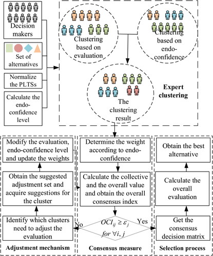
In order to intuitively reflect the consensus model based on endo-confidence, a visual procedure of the proposed model is presented in Figure 1.

Figure 1. The visual procedure of consensus decision-making model with endo-confidence.

Source: calculated by the methods using the original data.

4. Case study

4.1. Decision-making process with the proposed method

In order to prove the feasibility and efficiency of the decision-making model with endo-confidence factor proposed in this paper, a case study is given. In this case, there are four alternatives for experts to make decision which are denoted as $A=\{A_1,A_2,A_3,A_4\}.$ We ask experts to evaluate these alternatives from four attributes $C=\{c_1,c_2,c_3,c_4\}.$ The corresponding weights of each attribute are given as: $y_1=0.15,y_2=0.10,y_3=0.55,y_4=0.20.$ There are twenty experts $E=\{e^1,e^2,\dots ,e^{20}\}$ participated in the decision-making process, giving the corresponding probabilistic linguistic information $x_{ij}^a.$ Then, the decision matrix $X^a={[x_{ij}^a]}_{4\times 4}(a=1,2,\dots ,20)$ is generated randomly. In this case, we set $\alpha =0.4,$ $\beta =0.3,$ ${\chi }_{11,L(p)}=0.9,$ ${\chi }_{11,ec}=0.94$ and ${\epsilon }_1=0.88,$ ${\epsilon }_2=0.87,$ ${\epsilon }_3=0.84,$ ${\epsilon }_4=0.85.$

Step 1. Set $\varphi =0.$ We establish the endo-confidence level ($e{c}_{ij}^a$) of expert $e^a$ based on Section 3.1. The endo-confidence matrixes of experts are shown as follows: $$\begin{array}{c}{c}^1{c}^2{c}^3{c}^4\\ E{C}^1=\begin{array}{c}{A}_1\\ A_2\\ A_3\\ A_4\end{array}{\left[\begin{array}{cccc}0.4683& 0.3950& 0.3883& 0.6199\\ 0.5864& 0.3075& 0.3436& 0.5000\\ 0.5729& 0.5099& 0.5466& 0.5201\\ 0.5184& 0.4682& 0.3869& 0.5503\end{array}\right]}_{4\times 4},\dots ,E{C}^{20}=\begin{array}{c}{A}_1\\ A_2\\ A_3\\ A_4\end{array}{\left[\begin{array}{cccc}{c}^1& c^2& c^3& c^4\\ 0.5184& 0.9200& 0.5000& 0.6481\\ 0.7443& 0.4433& 0.5794& 0.8600\\ 0.7239& 0.5214& 0.6400& 0.6400\\ 0.4759& 0.9600& 0.5263& 0.3100\end{array}\right]}_{4\times 4}\end{array}$$

Step 2. We can obtain the normalised PLTSs by applying the method proposed in Section 3.2. We calculate the similarities of evaluation information among experts. Then, we obtain the order of the upper triangular elements of the similarity matrix (except the diagonal elements) as $1\ge 0.9745\ge$ $0.9647\ge \cdots \ge 0.2650.$ The optimal classification threshold ${\eta }_{11,L(p)}^{\ast }=0.9011$ is determined and the clustering results $G_{11,L(p)}$ are obtained. The similarities of the evaluation information are given below: $$\begin{array}{c}{e}^1{e}^2\cdots e^{20}\\ S{E}_{11}=\begin{array}{c}{e}^1\\ e^2\\ ⋮\\ e^{20}\end{array}{\left[\begin{array}{cccc}1& 0.7832& \cdots & 0.8545\\ & 1& \cdots & 0.6646\\ & & 1& ⋮\\ & & & 1\end{array}\right]}_{20\times 20}\end{array}$$

Subsequently, the similarity matrix of endo-confidence is established according to Equation (18)(18) $$se{c}_{ij}^{ab}(e{c}_{ij}^a,e{c}_{ij}^b)=1-|e{c}_{ij}^a-e{c}_{ij}^b|,a,b\in T$$(18) . Then, we can get the order of the upper triangular elements of the similarity matrix (except the diagonal elements) $1\ge 1\ge 1\ge \cdots \ge 0.5062.$ Thus, we get the optimal classification threshold ${\eta }_{11,ec}^{\ast }=0.94$ and obtain the clustering results $G_{11,ec}.$ $$\begin{array}{c}{e}^1{e}^2\cdots e^{20}\\ SE{C}_{11}=\begin{array}{c}{e}^1\\ e^2\\ ⋮\\ e^{20}\end{array}{\left[\begin{array}{cccc}1& 0.9584& \cdots & 0.9500\\ & 1& \cdots & 0.9915\\ & & 1& ⋮\\ & & & 1\end{array}\right]}_{20\times 20}\end{array}$$

The final clustering results $\overline{G_{11}}$ based on the results of the above two clustering results $G_{11,L(p)}$ and $G_{11,ec}$ are determined. The clustering results based on the similarities of evaluation information, the clustering results based on the similarities of endo-confidence levels and the final clustering results are shown in Table 1.

Table 1. The clustering results and the corresponding weights and endo-confidence levels.

$G_{11,L(p)}$	$e^a$	$\overline{G_{11}}$	$e^a$	$w_{11,\overline{G_{11,g}}}^{(0)}$	$e{c}_{11,\overline{G_{11,g}}}^{(0)}$
$G_{11,L{(p)}_1}$	$e^1,e^4,e^6,e^7,e^{13},e^{15},e^{17}$	$\overline{G_{11,1}}$	$e^1,e^4,e^6,e^7,e^{15},e^{17}$	0.3	0.4455
$G_{11,L{(p)}_2}$	$e^3,e^5,e^8,e^9,e^{10},e^{11},e^{16},e^{18},e^{20}$	$\overline{G_{11,2}}$	$e^3,e^5,e^8,e^{10},e^{20}$	0.25	0.5098
$G_{11,L{(p)}_3}$	$e^{12},e^{14}$	$\overline{G_{11,3}}$	$e^{11},e^{16},e^{18}$	0.15	0.6686
$G_{11,L{(p)}_4}$	$e^2,e^{19}$	$\overline{G_{11,4}}$	$e^2,e^{19}$	0.1	0.5099
$G_{11,ec}$	$e^a$	$\overline{G_{11,5}}$	$e^9$	0.05	0.8400
$G_{11,e{c}_1}$	$e^1,e^2,e^3,e^4,e^5,e^6,e^7,e^8,e^{10},e^{14},e^{15},e^{17},e^{19},e^{20}$	$\overline{G_{11,6}}$	$e^{12}$	0.05	0.6400
$G_{11,e{c}_2}$	$e^{11},e^{12},e^{13},e^{16},e^{18}$	$\overline{G_{11,7}}$	$e^{13}$	0.05	0.6968
$G_{11,e{c}_3}$	$e^9$	$\overline{G_{11,8}}$	$e^{14}$	0.05	0.4400

Source: calculated by the methods using the original data.

Step 3. The weight of each cluster $\overline{G_{11,g}}$ is shown in Table 1. To save space, the results for the weight of each expert $e^a$ in each cluster $\overline{G_{11,g}}$ are omitted here.

Step 4. We can get the collective evaluation information of the cluster $\overline{G_{11,g}}$ and the overall evaluation $\overline{L_{11}^{(0)}(p)}.$ Then, the overall consensus index$OC{I}_{11}^{(0)}=0.8348$ has been worked out. Compared with the consensus threshold ${\epsilon }_1=0.88,$ we can see that the consensus level is not reached. Then, some clusters need to adjust their evaluation information.

Step 5. We rank the clusters $\overline{G_{11,g}}$ according to their similarities and get $\overline{{G^{\prime }}_{11}}.$ Then, we choose cluster $\overline{G_{11,6}}$ to adjust the evaluation information. After calculating the endo-confidence level $e{c}_{11,\overline{G_{11,g}}}^{(0)}$ (see in Table 1), we get the suggested adjustment set $A{S}_{11,\overline{G_{11,g}}}^{(0)}=\{\overline{G_{11,3}},\overline{G_{11,5}},\overline{G_{11,7}}\}$ and further obtain the updated evaluation information and endo-confidence level of the cluster $\overline{G_{11,6}}.$

Step 6. Go back to Step 4. We calculate the overall evaluation and the overall consensus index, then, we compare with the consensus threshold ${\epsilon }_1=0.88$ to judge if the consensus level is reached. We get the overall consensus index for each iteration, that is $OC{I}_{11}^{(0)}=0.8348,$ $OC{I}_{11}^{(1)}=0.8338,$ $OC{I}_{11}^{(2)}=0.8500,$ $OC{I}_{11}^{(3)}=0.8651,$ $OC{I}_{11}^{(4)}=0.8661$ and $OC{I}_{11}^{(5)}=0.8850.$ The renewed weights $\overline{w_{11,\overline{G_{11,g}}}^{(\varphi )}}$ are shown in Table 2. Due to space limitations, the results of the suggestions and the updated evaluation information are omitted.

Table 2. The results of the updated weights.

$\overline{G_{11}}$	$\overline{w_{11,\overline{G_{11,g}}}^{(1)}}$	$\overline{w_{11,\overline{G_{11,g}}}^{(2)}}$	$\overline{w_{11,\overline{G_{11,g}}}^{(3)}}$	$\overline{w_{11,\overline{G_{11,g}}}^{(4)}}$	$\overline{w_{11,\overline{G_{11,g}}}^{(5)}}$
$\overline{G_{11,1}}$	0.1012	0.0998	0.0983	0.0975	0.0961
$\overline{G_{11,2}}$	0.1110	0.1095	0.1077	0.1069	0.1200
$\overline{G_{11,3}}$	0.1353	0.1335	0.1314	0.1379	0.1359
$\overline{G_{11,4}}$	0.1110	0.1095	0.1235	0.1226	0.1208
$\overline{G_{11,5}}$	0.1630	0.1608	0.1583	0.1571	0.1548
$\overline{G_{11,6}}$	0.1383	0.1364	0.1342	0.1332	0.1313
$\overline{G_{11,7}}$	0.1397	0.1378	0.1357	0.1346	0.1327
$\overline{G_{11,8}}$	0.1004	0.1127	0.1109	0.1101	0.1085

Source: calculated by the methods using the original data.

Step 7. After five iterations, the consensus for the alternative $A_1$ over the attribute $c_1$ has been reached. After the consensus achieved for $\forall i,j,$ we obtain the overall evaluation $\overline{L_i(p)},$ and get the corresponding score $E(\overline{L_i(p)}).$ That is $E(\overline{L_1(p)})=s_{3.0851},$ $E(\overline{L_2(p)})=s_{2.9427},$ $E(\overline{L_3(p)})=s_{2.7630}$ and $E(\overline{L_4(p)})=s_{3.0749}.$ Finally, we get the best alternative $A_1.$

4.2. The decision-making method without considering the endo-confidence of DMs

In this paper, we proposed a decision-making model for LSGDM considering the endo-confidence in PLTSs. In order to demonstrate the influence of endo-confidence factors on the decision-making process, here we give a decision-making model without endo-confidence level. The detailed steps are depicted as follows:

Step 1. Set $\varphi =0.$ We convert the original evaluation information into the complete PLTSs according to the method proposed in Section 3.2.

Step 2. Get the similarities of evaluation information by Equation (5)(5) $$\rho (\overline{L^1(p)},\overline{L^2(p)})=1-d(\overline{L^1(p)},\overline{L^2(p)})$$(5) , and use it to distinguish the experts based on Section 3.3. We can obtain the clusters $G_{ij,L(p)}=\{G_{ij,L{(p)}_1},G_{ij,L{(p)}_2},\dots ,G_{ij,L{(p)}_g},\dots ,G_{ij,L{(p)}_{\overline{\xi }}}\}$ and take it as the final clustering results, denoted as $\overline{G_{ij}}=\{\overline{G_{ij,1}},\overline{G_{ij,2}},\dots ,\overline{G_{ij,g}},\dots ,\overline{G_{ij,\sigma }}\}.$

Step 3. Based on the majority principle, we calculate the weight $\overline{w_{ij,\overline{G_{ij,g}}}^a}$ of the experts $e^a$ in each cluster $\overline{G_{ij,g}}:$ (39) $$\overline{w_{ij,\overline{G_{ij,g}}}^a}=\frac{1}{\#N{E}_{\overline{G_{ij.g}}}}$$(39)

Further, according to Equation (23)(23) $$\overline{w_{ij,\overline{G_{ij,g}}}}=\frac{\#N{E}_{\overline{G_{ij.g}}}}{\sum _{g=1}^{\sigma }\#N{E}_{\overline{G_{ij.g}}}}$$(23) , we get the weight $\overline{w_{ij,\overline{G_{ij,g}}}}$ of each cluster $\overline{G_{ij,g}}.$

Step 4. Get the collective and overall evaluation information by utilising Equations (24)–(27), and we can obtain the overall consensus index $OC{I}_{ij}.$ Judge the consensus has been reached or not by comparing $OC{I}_{ij}$ with the threshold ${\epsilon }_j.$ If the consensus level is achieved, then, go to Step 6; otherwise, go to Step 5. If all the clusters have adjusted their evaluation information and the consensus has not been reached yet, the consensus fails and the decision-making process should be terminated.

Step 5. Rank the clusters $\overline{G_{ij,g}}$ according to the similarities $\rho (\overline{L_{ij,\overline{G_{ij,g}}}(p)},\overline{L_{ij}(p)})$ and choose the cluster with the smallest similarity to adjust the evaluation until the consensus reaches. We adjust the evaluation information according to the collective information $\overline{L_{ij}(p)}.$ Notice that, each cluster $\overline{G_{ij,g}}$ can only adjust the evaluation once.

After $\varphi$ iterations, we obtain the rearranged PLTS ${\overline{L_{ij,\overline{G_{ij,g}}}(p)}}^{\ast (\varphi )}=\{{\overline{L_{ij,\overline{G_{ij,g}}}^{(k^{\prime })}}}^{(\varphi )}({\overline{p_{ij}^{(k^{\prime })}}}^{\ast }{}^{(\varphi )})$ $|k^{\prime }=1,2,\dots ,\#{\overline{L_{ij,\overline{G_{ij,g}}}(p)}}^{\ast }{}^{(\varphi )}\}$ of the collective evaluation information ${\overline{L_{ij,\overline{G_{ij,g}}}(p)}}^{(\varphi )}$ and the rearranged PLTS ${\overline{L_{ij}(p)}}^{\ast (\varphi )}=\{{\overline{L_{ij}^{(k^{\prime })}}}^{(\varphi )}({\overline{p_{ij}^{(k^{\prime })}}}^{\ast (\varphi )})|k^{\prime }=1,2,\dots ,\#{\overline{L_{ij}(p)}}^{\ast (\varphi )}\}$ of the overall evaluation ${\overline{L_{ij}(p)}}^{(\varphi )}$ according to the method in Section 2.2.

Then, the updated evaluation information of the cluster $\overline{G_{ij,g}}$ can be calculated by Equation (40)(40) $$\begin{array}{c}{\overline{L_{ij,\overline{G_{ij,g}}}(p)}}^{(\varphi +1)}=\frac{1}{2}\cdot {\overline{L_{ij,\overline{G_{ij,g}}}(p)}}^{\ast (\varphi )}+\frac{1}{2}\cdot {\overline{L_{ij}(p)}}^{*(\varphi )}\\ =\{{\overline{L_{ij,\overline{G_{ij,g}}}^{(k^{\prime })}}}^{(\varphi +1)}({\overline{p_{ij,\overline{G_{ij,g}}}^{(k^{\prime })}}}^{(\varphi +1)})|{\overline{p_{ij,\overline{G_{ij,g}}}^{(k^{\prime })}}}^{(\varphi +1)}\ge 0,\sum _{k^{\prime }=1}^{\#{\overline{L_{ij,\overline{G_{ij,g}}}(p)}}^{(\varphi +1)}}{\overline{p_{ij,\overline{G_{ij,g}}}^{(k^{\prime })}}}^{(\varphi +1)}=1\}\end{array}$$(40) : (40) $$\begin{array}{c}{\overline{L_{ij,\overline{G_{ij,g}}}(p)}}^{(\varphi +1)}=\frac{1}{2}\cdot {\overline{L_{ij,\overline{G_{ij,g}}}(p)}}^{\ast (\varphi )}+\frac{1}{2}\cdot {\overline{L_{ij}(p)}}^{*(\varphi )}\\ =\{{\overline{L_{ij,\overline{G_{ij,g}}}^{(k^{\prime })}}}^{(\varphi +1)}({\overline{p_{ij,\overline{G_{ij,g}}}^{(k^{\prime })}}}^{(\varphi +1)})|{\overline{p_{ij,\overline{G_{ij,g}}}^{(k^{\prime })}}}^{(\varphi +1)}\ge 0,\sum _{k^{\prime }=1}^{\#{\overline{L_{ij,\overline{G_{ij,g}}}(p)}}^{(\varphi +1)}}{\overline{p_{ij,\overline{G_{ij,g}}}^{(k^{\prime })}}}^{(\varphi +1)}=1\}\end{array}$$(40) where (41) $$\begin{array}{c}{\overline{L_{ij,\overline{G_{ij,g}}}^{(k^{\prime })}}}^{(\varphi +1)}=f^{-1}(\frac{1}{2}\cdot f({\overline{L_{ij,\overline{G_{ij,g}}}^{(k^{\prime })}}}^{(\varphi )})+\frac{1}{2}\cdot f({\overline{L_{ij}^{(k^{\prime })}}}^{(\varphi )})),{\overline{p_{ij,\overline{G_{ij,g}}}^{(k^{\prime })}}}^{(\varphi +1)}={\overline{p_{ij}^{(k^{\prime })}}}^{\ast (\varphi )}\\ k^{\prime }=1,2,\dots ,\#{\overline{L_{ij,\overline{G_{ij,g}}}(p)}}^{(\varphi +1)}\text{and}\#{\overline{L_{ij,\overline{G_{ij,g}}}(p)}}^{\ast (\varphi )}=\#{\overline{L_{ij}(p)}}^{\ast (\varphi )}=\#{\overline{L_{ij,\overline{G_{ij,g}}}(p)}}^{(\varphi +1)}.\end{array}$$(41)

For other clusters $\overline{G_{ij,g^{″}}}$ that do not need to adjust their evaluation information, we can also get ${\overline{L_{ij,\overline{G_{ij,g^{″}}}}(p)}}^{(\varphi +1)}:$ (42) $${\overline{L_{ij,\overline{G_{ij,g^{″}}}}(p)}}^{(\varphi +1)}={\overline{L_{ij,\overline{G_{ij,g^{″}}}}(p)}}^{(\varphi )}$$(42)

We keep the weight of each cluster unchanged, that is $\overline{w_{ij,\overline{G_{ij,g}}}^{(\varphi +1)}}=\overline{w_{ij,\overline{G_{ij,g}}}^{(\varphi )}}=\frac{\#N{E}_{\overline{G_{ij.g}}}}{{\sum }_{g=1}^{\sigma }\#N{E}_{\overline{G_{ij.g}}}}.$ Then, let $\varphi =\varphi +1$ and repeat Step 4.

Step 6. Get the consensus evaluation information and obtain the overall evaluation $\overline{L_i(p)}$ based on Equation (37)(37) $$\overline{L_i(p)}=\underset{j=1}{\overset{m}{\oplus }}{y}_j\cdot {\overline{L_{ij}(p)}}^{\ast (\varphi )}=\{\overline{L_i^{(k^{\prime })}}(\overline{p_i^{(k^{\prime })}})|\overline{p_i^{(k^{\prime })}}\ge 0,\sum _{k^{\prime }=1}^{\#\overline{L_i(p)}}\overline{p_i^{(k^{\prime })}}=1\}$$(37) . Then, we calculate the score $E(\overline{L_i(p)})$ of the overall evaluation $\overline{L_i(p)},$ rank and find the best alternative.

4.3. Comparative analysis

In order to prove that the model proposed in Section 3 can reflect the influence of endo-confidence on decision-making process, we change the values of the parameters $\alpha$ and $\beta$ to reflect the effect of different importance degrees of endo-confidence measurement on the decision results. We make a comparison between the clustering results, the final weights of the cluster $\overline{G_{11,g}},$ the overall consensus index $OC{I}_{11}$ and the final decision results. The same data and other parameters in Section 4.1 are utilised. We first set the parameters $\alpha =0.4,$ $\beta =0.3$ and denote it as Model I with Case I. Then, the parameters become $\alpha =0.2$ and $\beta =0.5$ which is named as Model I with Case II. We can see the detailed results of the above two cases in Table 3.

Table 3. The comparative results of Model I (case I and case II) and Model II.

	Model I with case I		Model I with case II		Model II
$\overline{G_{11}}$	$e^a$	$\overline{w_{11,\overline{G_{11,g}}}^{(5)}}$	$e^a$	$\overline{w_{11,\overline{G_{11,g}}}^{(6)}}$	$e^a$	$\overline{w_{11,\overline{G_{11,g}}}^{(3)}}$
$\overline{G_{11,1}}$	$e^1,e^4,e^6,e^7,e^{15},e^{17}$	0.0961	$e^1,e^6,e^7,e^{15},e^{17}$	0.0649	$e^1,e^4,e^6,e^7,e^{13},e^{15},e^{17}$	0.35
$\overline{G_{11,2}}$	$e^3,e^5,e^8,e^{10},e^{20}$	0.1200	$e^3,e^5,e^8,e^{20}$	0.0970	$e^3,e^5,e^8,e^9,e^{10},e^{11},e^{16},e^{18},e^{20}$	0.45
$\overline{G_{11,3}}$	$e^{11},e^{16},e^{18}$	0.1359	$e^{10},e^{11},e^{16}$	0.1090	$e^{12},e^{14}$	0.1
$\overline{G_{11,4}}$	$e^2,e^{19}$	0.1208	$e^2,e^{19}$	0.0905	$e^2,e^{19}$	0.1
$\overline{G_{11,5}}$	$e^9$	0.1548	$e^9$	0.1392
$\overline{G_{11,6}}$	$e^{12}$	0.1313	$e^{12}$	0.1323
$\overline{G_{11,7}}$	$e^{13}$	0.1327	$e^{13}$	0.1067
$\overline{G_{11,8}}$	$e^{14}$	0.1085	$e^{14}$	0.0977
$\overline{G_{11,9}}$			$e^{18}$	0.1152
$\overline{G_{11,10}}$			$e^4$	0.0475
	$\overline{{\upsilon }^i}$	Rank	$\overline{{\upsilon }^i}$	Rank	$\overline{{\upsilon }^i}$	Rank
$A_1$	3.0851	1	3.0988	1	3.0689	2
$A_2$	2.9427	3	2.9437	3	2.9437	3
$A_3$	2.7630	4	2.7694	4	2.7744	4
$A_4$	3.0749	2	3.0790	2	3.0791	1

Source: calculated by the methods using the original data.

Table A1. The meaning of notations used in the proposed model.

Notation	Meaning
$\overline{L}=\{s_l,\dots ,s_{\gamma },\dots ,s_u\}$	The normalised LTS, where $s_l$ and $s_u$ represent the lower and upper bounds of the normalised LTS respectively
$\overline{L(p_{\varsigma })}=\{\overline{L^{(k^{\prime })}}(p_{\varsigma }^{(k^{\prime })})|p_{\varsigma }^{(k^{\prime })}\ge 0,k^{\prime }=1,2,\dots ,\#\overline{L(p_{\varsigma })},{\sum }_{k^{\prime }=1}^{\#\overline{L(p_{\varsigma })}}{p}_{\varsigma }^{(k^{\prime })}\le 1\}$	The PLTS with the expanded original information
$\overline{h(p^{(k^{\prime })})}$	The normalised proportion of the probability distribution
$\overline{L(p)}=\{\overline{L^{(k^{\prime })}}(\overline{p^{(k^{\prime })}})|\overline{p^{(k^{\prime })}}\ge 0,k^{\prime }=1,2,\dots ,\#\overline{L(p)},{\sum }_{k^{\prime }=1}^{\#\overline{L(p)}}\overline{p^{(k^{\prime })}}=1\}$	The normalised PLTS
$E=\{e^1,e^2,\dots ,e^t\}$ ($T=\{1,2,\dots ,t\},$ $a\in T,$ $t\ge 20$)	The finite set of experts
$A=\{A_1,A_2,\dots ,A_n\}$ ($N=\{1,2,\dots ,n\},$ $i\in N,$ $n\ge 3$)	The finite set of potential alternatives
$C=\{c_1,c_2,\dots ,c_m\}$ ($M=\{1,2,\dots ,m\},$ $j\in M,$ $m\ge 2$)	The finite set of attributes
$e{c}^a$	The endo-confidence level of the expert $e^a$
$e{c}_p$	The endo-confidence level from the perspective of total probability
$e{c}_h$	The endo-confidence level based on hesitation
$e{c}_d$	The endo-confidence level from the perspective of preference among linguistic terms
$G_{ij,L(p)}=\{G_{ij,L{(p)}_1},G_{ij,L{(p)}_2},\dots ,G_{ij,L{(p)}_g},\dots ,G_{ij,L{(p)}_{\overline{\xi }}}\}$	The clusters of DMs based on the similarities of evaluation information
$G_{ij,ec}=\{G_{ij,e{c}_1},G_{ij,e{c}_2},\dots ,G_{ij,e{c}_g},\dots ,G_{ij,e{c}_{\overline{\xi }}}\}$	The clusters of DMs based on the similarities of endo-confidence levels among DMs
$\overline{G_{ij}}=\{\overline{G_{ij,1}},\overline{G_{ij,2}},\dots ,\overline{G_{ij,g}},\dots ,\overline{G_{ij,\sigma }}\}$	The final clustering results
${\eta }_{ij,L(p)}^{\ast }$/${\eta }_{ij,ec}^{\ast }$	The optimal classification threshold which is determined by the maximum value of the classification threshold ${{\eta }^{\prime }}_{ij,L(p)}$/${{\eta }^{\prime }}_{ij,ec}$ and the threshold ${\chi }_{ij,L(p)}$/${\chi }_{ij,ec}$ given by DMs
$\overline{w_{ij,\overline{G_{ij,g}}}}$	The weight of the cluster $\overline{G_{ij,g}}$
$\overline{w_{ij,\overline{G_{ij,g}}}^a}$	The weight of the expert $e^a$ in the cluster $\overline{G_{ij,g}}$
${\overline{L_{ij,\overline{G_{ij,g}}}^a(p)}}^{\ast }=\{\overline{L_{ij,\overline{G_{ij,g}}}^{a(k^{\prime })}}({\overline{p_{ij,\overline{G_{ij,g}}}^{(k^{\prime })}}}^{\ast })|k^{\prime }=1,2,\dots ,\#{\overline{L_{ij,\overline{G_{ij,g}}}^a(p)}}^{\ast }\}$	The rearranged PLTSs of the evaluation given by the expert $e^a$ in the cluster $\overline{G_{ij,g}}$
$\overline{L_{ij,\overline{G_{ij,g}}}(p)}$	The collective evaluation information of the cluster $\overline{G_{ij,g}}$
${\overline{L_{ij,\overline{G_{ij,g}}}(p)}}^{\ast }=\{\overline{L_{ij,\overline{G_{ij,g}}}^{(k^{\prime })}}({\overline{p_{ij}^{(k^{\prime })}}}^{\ast })|k^{\prime }=1,2,\dots ,\#{\overline{L_{ij,\overline{G_{ij,g}}}(p)}}^{\ast }\}$	The rearranged PLTS of the collective evaluation information $\overline{L_{ij,\overline{G_{ij,g}}}(p)}$ in the cluster $\overline{G_{ij,g}}$
$\overline{L_{ij}(p)}$	The overall evaluation
$OC{I}_{ij}$	The overall consensus index
$\overline{{G^{\prime }}_{ij,g}}$	The order of the clusters obtained by sorting the similarities ${\rho }_{ij,\overline{G_{ij,g}}}$
$e{c}_{ij,\overline{G_{ij,g}}}$	The endo-confidence level of the cluster $\overline{G_{ij,g}}$
$A{S}_{ij,\overline{G_{ij,g}}}=\left\{\overline{G_{ij,g^{\prime }}}\right|e{c}_{ij,\overline{G_{ij,g^{\prime }}}}\ge e{c}_{ij,\overline{G_{ij,g}}},g^{\prime }\ne g\}$	The suggested adjustment set
$\overline{w_{ij,\overline{G_{ij,g^{\prime }}}}}$	The weight of the cluster $\overline{G_{ij,g^{\prime }}}$ in $A{S}_{ij,\overline{G_{ij,g}}}$
${\overline{L_{ij,\overline{G_{ij,g^{\prime }}}}(p)}}^{\ast }=\{\overline{L_{ij,\overline{G_{ij,g^{\prime }}}}^{(k^{\prime })}}({\overline{p_{ij}^{(k^{\prime })}}}^{\ast })|k^{\prime }=1,2,\dots ,\#{\overline{L_{ij,\overline{G_{ij,g^{\prime }}}}(p)}}^{\ast }\}$	The rearranged PLTSs of the collective evaluation information $\overline{L_{ij,\overline{G_{ij,g^{\prime }}}}(p)}$ in the suggested adjustment set $A{S}_{ij,\overline{G_{ij,g}}}$
$\overline{L_{\mathit{ijA}{S}_{ij,\overline{G_{ij,g}}}}(p)}=\{\overline{L_{\mathit{ijA}{S}_{ij,\overline{G_{ij,g}}}}^{(k^{\prime })}}(\overline{p_{\mathit{ijA}{S}_{ij,\overline{G_{ij,g}}}}^{(k^{\prime })}})|\overline{p_{\mathit{ijA}{S}_{ij,\overline{G_{ij,g}}}}^{(k^{\prime })}}\ge 0,{\sum }_{k^{\prime }=1}^{\#\overline{L_{\mathit{ijA}{S}_{ij,\overline{G_{ij,g}}}}(p)}}\overline{p_{\mathit{ijA}{S}_{ij,\overline{G_{ij,g}}}}^{(k^{\prime })}}=1\}$	Part of the suggestions for the cluster $\overline{G_{ij,g}}$
${\overline{L_{ij,\overline{G_{ij,g}}}(p)}}^{(\varphi )}=\{{\overline{L_{ij,\overline{G_{ij,g}}}^{(k^{\prime })}}}^{(\varphi )}({\overline{p_{ij,\overline{G_{ij,g}}}^{(k^{\prime })}}}^{(\varphi )})|{\overline{p_{ij,\overline{G_{ij,g}}}^{(k^{\prime })}}}^{(\varphi )}\ge 0,{\sum }_{k^{\prime }=1}^{\#{\overline{L_{ij,\overline{G_{ij,g}}}(p)}}^{(\varphi )}}{\overline{p_{ij,\overline{G_{ij,g}}}^{(k^{\prime })}}}^{(\varphi )}=1\}$	The updated evaluation information of the cluster $\overline{G_{ij,g}}$ in the $\varphi$-th round
$e{c^{\prime }}_{ij,\overline{G_{ij,g}}}$	The average endo-confidence level of the cluster $\overline{G_{ij,g^{\prime }}}$ in the suggested adjustment set $A{S}_{ij,\overline{G_{ij,g}}}$
$e{c}_{ij,\overline{G_{ij,g}}}^{(\varphi )}$	The updated endo-confidence level of the cluster $\overline{G_{ij,g}}$ in the $\varphi$-th round
$\overline{w_{ij,\overline{G_{ij,g}}}^{(\varphi )}}$	The updated weight for the cluster $\overline{G_{ij,g}}$ in the $\varphi$-th round
${\overline{L_{ij}(p)}}^{\ast (\varphi )}=\{{\overline{L_{ij}^{(k^{\prime })}}}^{(\varphi )}({\overline{p_i^{(k^{\prime })}}}^{\ast (\varphi )})|k^{\prime }=1,2,\dots ,\#{\overline{L_{ij}(p)}}^{\ast (\varphi )}\}$	The rearranged PLTSs of the consensus decision information ${\overline{L_{ij}(p)}}^{(\varphi )}$
$\overline{L_i(p)}$	The overall evaluation of the alternative $A_i$
$E(\overline{L_i(p)})$	The score of the overall evaluation $\overline{L_i(p)}$

Source: calculated by the methods using the original data.

According to Table 3, we can find that in Case I, the expert $e^{10}$ is the neighbor of experts $e^3$ $e^5,$ $e^8$ and $e^{20},$ while the expert $e^{10}$ is distinguished into one cluster with the experts $e^{11}$ and $e^{16}$ in Case II. In the two cases, the similarities of the evaluation information have not changed. Hence, the difference in clustering results is entirely caused by the difference of the similarities of endo-confidence levels. In other words, the similarity-based clustering algorithm takes both evaluation information and endo-confidence levels into consideration, and the clustering results are more reasonable. Moreover, as we can see in Table 3, we have different updated weights $\overline{w_{11,\overline{G_{11,g}}}^{(\varphi )}}$ due to different clustering results and different modified endo-confidence levels of the cluster $\overline{G_{11,g}}.$ Furthermore, the overall consensus indexes of Case I and Case II equal to $OC{I}_{11}^{(0)}=0.8348$ and $OC{I}_{11}^{(0)}=0.8327$ respectively. We can conclude that under different endo-confidence levels, there are differences in the overall consensus index due to the different collective evaluation information of each cluster and the differences in its corresponding weights. The overall consensus indexes of Case I and Case II after modification are $OC{I}_{11}^{(5)}=0.8850$ and $OC{I}_{11}^{(6)}=0.8898$ respectively. Notice that, the changes in the overall consensus index $\Delta OC{I}_{11}=OC{I}_{11}^{(\varphi )}-OC{I}_{11}^{(0)}$ are significantly different under Case I and Case II, that is ${\Delta }_{I}OC{I}_{11}=0.0502$ and ${\Delta }_{II}OC{I}_{11}=0.0571$ respectively. Thus, we can conclude that the feedback mechanism which considers both evaluation information and endo-confidence levels make sense. The final result of both Case I and Case II is $A_1\succ A_4\succ A_2\succ A_3.$ Although the above two cases conclude in the same result, their scores of the overall evaluation are different. We can find that the parameters $\alpha$ and $\beta$ are sensitive to the decision result.

Furthermore, we make a comparison among Model I (with Case I and Case II) and Model II proposed in Section 4.2. In the clustering process, Model II does not consider the similarities of endo-confidence levels. Hence, the experts with different characteristic are divided into one cluster (see the experts $e^3,e^5,e^8,e^9,e^{10},e^{11},$ $e^{16},e^{18},e^{20}$) which may lead to biased decision results. The weight $\overline{w_{11,\overline{G_{11,g}}}^{(3)}}$ of Model II is always determined by the number of experts in the cluster $\overline{G_{11,g}}.$ On the one hand, the determination of the weights does not consider the psychological factor. On the other hand, the weights could not be flexibly adjusted during the interaction process. After three iterations, the overall consensus index $OC{I}_{11}^{(3)}=0.8839$ and the consensus level is reached. Although Model II can reach consensus in fewer rounds, it will cause more information loss in each round of adjustment. Notice that the final result of Model II is $A_4\succ A_1\succ A_2\succ A_3,$ which is different from the result of Model I. It is obvious that endo-confidence has an impact on decision-making results. Thus, it is necessary to consider experts’ endo-confidence levels when making decisions and the model proposed in this paper has great value and practical significance.

5. Conclusions

In this paper, we propose a decision-making process under PLTSs which considers the endo-confidence levels of DMs. A method to determine the endo-confidence level of each DM from his/her evaluation information is given. We give a novel way to normalise the PLTSs which holds more original information. The similarity-based clustering algorithm is utilised to distinguish the experts into different clusters according to the similarities of both evaluation information and endo-confidence levels. Then, the relationship between endo-confidence and weight is discussed. Motivated by hyperbolic sine function, the weight determination method is proposed. Subsequently, we present the consensus measurement to calculate the overall consensus index and the feedback adjustment mechanism, which can help clusters adjust their evaluation information to reach the consensus level. Also, we give the selection process to choose the best alternative with the consensus evaluation information.

Although the proposed consensus model with endo-confidence has its advantage, sometimes, the single form of evaluation information could not properly describe all the attributes of alternatives. Hence, the consensus based on endo-confidence with heterogeneous evaluation information should be discussed in the future. Also, non-cooperative behaviour is also hot topic in the consensus problem (Gou, Xu, Liao, et al., 2021), and self-confidence have an influence on the degree of non-cooperative behaviour. As a result, considering the effect of endo-confidence on the non-cooperative behaviour in consensus model is another topic in our future study. Moreover, sometimes it is not easy for us to directly obtain sufficient eloquent data in the form of PLTSs. Hence, in the future, we may study the method to extract PLTSs from the natural language by using natural language processing technology, and give the applications of the decision method presented in this paper.

Disclosure statement

No potential conflict of interest was reported by the authors.

Additional information

Funding

The work was supported in part by the Fundamental Research Funds for the Central Universities (JBK2101044).

Notes

1 It is worth mentioning that, the hyperbolic sine function is not the only function that satisfies these conditions.

Appendix

In order to facilitate readers to understand the normalisation method, the clustering procedure and the weight determination method with endo-confidence, we give the following examples in Appendix.

Example 3.

Let $L^1(p)=\{s_4(0.4),s_5(0.5)\}$ and $L^2(p)=\{s_4(0.1),s_5(0.2)\}$ be two PLTSs. According to (2(2) $$E(L(p))=s_{\overline{\upsilon }}$$(2) ), there is $\overline{{\upsilon }^1}=(4\times 0.4+5\times 0.5)/(0.4+0.5)\approx 4.56,$ $E(L^1(p))=s_{4.56}$ and $\overline{{\upsilon }^2}=(4\times 0.1+5\times$ $0.2)/(0.1+0.2)\approx 4.67,$ $E(L^2(p))=s_{4.67}.$ The lower bounds of the normalised PLTS $s_{3.65}$ can be calculated by $l^1=\max [-\frac{1}{2}\times (1-0.9)\times 7+4,0]=3.65,$ and the upper bounds of the normalised PLTS $s_{5.35}$ can be calculated by $u^1=\min [\frac{1}{2}\times (1-0.9)\times 7+5,6]=5.35.$ Then, the normalised LTS is denoted as $\overline{L^1}=\{s_{3.65},s_4,s_5,s_{5.35}\}.$ Similarly, we can obtain the normalised LTS of $L^2(p)$ as $\overline{L^2}=\{s_{1.55},s_2,s_3,s_4,s_5,s_6\}.$ Then, we compare each terms in PLTS $\overline{L^1(p_{\varsigma })}$ with its score, and use Equation (14)(14) $$h(p^{(k^{\prime })})=\{\begin{array}{c}\hspace{0.17em}\text{exp}\hspace{0.17em}({\gamma }^{(k^{\prime })})ifl\le {\gamma }^{(k^{\prime })}\le \overline{\upsilon }\\ \hspace{0.17em}\text{exp}[2\cdot \overline{\upsilon }-{\gamma }^{(k^{\prime })}]if\overline{\upsilon }<{\gamma }^{(k^{\prime })}\le u\end{array}$$(14) to calculate the proportion of probability distribution $h(p^{1(k^{\prime })}).$ As $3.65<4<4.56,$ we can obtain $h(p^{1(1)})=\hspace{0.17em}\text{exp}\hspace{0.17em}(3.65)\approx 38.475$ and $h(p^{1(2)})=\hspace{0.17em}\text{exp}\hspace{0.17em}(4)\approx 54.598.$ Similarly, we can find that $4.56<5<5.35,$ the proportion of probability distribution are $h(p^{1(3)})=\hspace{0.17em}\text{exp}\hspace{0.17em}(2\times 4.56-5)\approx 61.559$ and $h(p^{1(4)})=\hspace{0.17em}\text{exp}\hspace{0.17em}(2\times 4.56$ $-5.35)\approx 43.380.$ Then, we apply Equation (15)(15) $$\overline{h(p^{(k^{\prime })})}=\frac{h(p^{(k^{\prime })})}{\sum _{k^{\prime }=1}^{\#\overline{L(p_{\varsigma })}}h(p^{(k^{\prime })})}$$(15) to get the normalised proportion of probability distribution $\overline{h(p^{1(k^{\prime })})},$ which is $\overline{h(p^{1(1)})}=38.475/198.012\approx 0.194,$ $\overline{h(p^{1(2)})}\approx 0.276,$ $\overline{h(p^{1(3)})}\approx 0.311$ and $\overline{h(p^{1(4)})}\approx 0.219.$ Subsequently, we use Equation (16)(16) $$\overline{p^{(k^{\prime })}}=\overline{h(p^{(k^{\prime })})}\cdot (1-{\sum }_{k^{\prime }=1}^{\#\overline{L(p_{\varsigma })}}{p}_{\varsigma }^{(k^{\prime })})+p_{\varsigma }^{(k^{\prime })},\mathrm{}\sum _{k^{\prime }=1}^{\#\overline{L(p)}}\overline{p^{(k^{\prime })}}=1$$(16) to obtain the normalised probabilities $\overline{p^{1(1)}}=0.194\cdot 0.1+0\approx 0.019,$ $\overline{p^{1(2)}}\approx 0.428,$ $\overline{p^{1(3)}}\approx 0.531$ and $\overline{p^{1(4)}}\approx 0.022.$ Finally, the normalised PLTS is $\overline{L^1(p)}=\{s_{3.65}(0.019),$ $s_4(0.428),s_5(0.531),s_{5.35}(0.022)\}.$ For $L^2(p),$ we can get the normalised PLTS in the same way as $\overline{L^2(p)}=\{s_{1.55}(0.017),s_2(0.027),s_3(0.073),s_4(0.3),s_5(0.480),s_6(0.103)\}.$

Example 4.

Suppose that the upper matrix of similarities of five experts based on the alternative $A_1$ over the attribute $c_1$ is: $$\begin{array}{c}{e}^1{e}^2{e}^3{e}^4{e}^5\\ S{E}_{11}=\begin{array}{c}{e}^1\\ e^2\\ e^3\\ \begin{array}{c}{e}^4\\ e^5\end{array}\end{array}{\left[\begin{array}{ccccc}1& 0.86& 0.91& 0.83& 0.97\\ & 1& 0.93& 0.99& 0.96\\ & & 1& 0.81& 0.98\\ & & & 1& 0.87\\ & & & & 1\end{array}\right]}_{5\times 5}\end{array}$$

Then, ${\eta }_{11,L{(p)}_1}(e^2{e}^4)=0.99>{\eta }_{11,L{(p)}_2}(e^3{e}^5)=0.98>{\eta }_{11,L{(p)}_3}(e^1{e}^5)=0.97>{\eta }_{11,L{(p)}_4}(e^2{e}^5)=0.96>{\eta }_{11,L{(p)}_5}(e^2{e}^3)=0.93$ $>{\eta }_{11,L{(p)}_6}(e^1{e}^3)=0.91>{\eta }_{11,L{(p)}_7}(e^4{e}^5)=0.87>{\eta }_{11,L{(p)}_8}(e^1{e}^2)=0.86>{\eta }_{11,L{(p)}_9}(e^1{e}^4)=0.83>{\eta }_{11,L{(p)}_{10}}(e^3{e}^4)=0.81.$ When ${\eta }_{11,L{(p)}_3}=0.97,$ all the fives experts are involved in cluster, then, the classification threshold ${{\eta }^{\prime }}_{11,L(p)}=0.97.$ Then we get the optimal classification threshold ${\eta }_{11,L(p)}^{\ast }=\max (0.97,0.9)=0.97.$ Considering this, there are two clusters as: $G_{11,L{(p)}_1}=\{e^2,e^4\}$ and $G_{11,L{(p)}_2}=\{e^1,e^3,e^5\}.$

Suppose that the upper matrix of similarities of endo-confidence levels of five experts based on the alternative $A_1$ over the attribute $c_1$ is: $$\begin{array}{c}{e}^1{e}^2{e}^3{e}^4{e}^5\\ SE{C}_{11}=\begin{array}{c}{e}^1\\ e^2\\ e^3\\ \begin{array}{c}{e}^4\\ e^5\end{array}\end{array}{\left[\begin{array}{ccccc}1& 0.82& 0.97& 0.81& 0.93\\ & 1& 0.88& 0.95& 0.91\\ & & 1& 0.79& 0.92\\ & & & 1& 0.84\\ & & & & 1\end{array}\right]}_{5\times 5}\end{array}$$

Then, ${\eta }_{11,e{c}_1}(e^1{e}^3)=0.97>{\eta }_{11,e{c}_2}(e^2{e}^4)=0.95>{\eta }_{11,e{c}_3}(e^1{e}^5)=0.93>{\eta }_{11,e{c}_4}(e^3{e}^5)=0.92>{\eta }_{11,e{c}_5}(e^2{e}^5)=0.91>$ ${\eta }_{11,e{c}_6}(e^2{e}^3)=0.88>{\eta }_{11,e{c}_7}(e^4{e}^5)=0.84>{\eta }_{11,e{c}_8}(e^1{e}^2)=0.82>{\eta }_{11,e{c}_9}(e^1{e}^4)=0.81>{\eta }_{11,e{c}_{10}}(e^3{e}^4)=0.79.$ We can get ${{\eta }^{\prime }}_{11,ec}=0.93.$ Then, the optimal classification threshold ${\eta }_{11,ec}^{\ast }=\max (0.93,0.94)=0.94.$ Considering this, there are three clusters as: $G_{11,e{c}_1}=\{e^2,e^4\},$ $G_{11,e{c}_2}=\left\{e^5\right\}$ and $G_{11,e{c}_3}=\{e^1,e^3\}.$

According to the above clustering results based on evaluation and endo-confidence levels, we can see that $G_{11,L{(p)}_1}\cap G_{11,e{c}_1}=\{e^2,e^4\},$ $G_{11,L{(p)}_2}\cap G_{11,e{c}_3}=\{e^1,e^3\}$ and $G_{11,L{(p)}_2}\cap G_{11,e{c}_2}=\left\{e^5\right\}.$ As a result, we can finally acquire the final clustering results as $\overline{G_{11,1}}=\{e^1,e^3\},$ $\overline{G_{11,2}}=\left\{e^5\right\}$ and $\overline{G_{11,3}}=\{e^2,e^4\}.$

Example 5.

If there are six experts in the cluster $\overline{G_{11,g}}$ whose endo-confidence levels are $e{c}_{11,\overline{G_{11,g}}}^1=0.1,$ $e{c}_{11,\overline{G_{11,g}}}^2=0.2,$ $e{c}_{11,\overline{G_{11,g}}}^3=0.45,$ $e{c}_{11,\overline{G_{11,g}}}^4=0.55,$ $e{c}_{11,\overline{G_{11,g}}}^5=0.8$ and $e{c}_{11,\overline{G_{11,g}}}^6=0.9.$ First, we use Equation (21)(21) $$\overline{e{c}_{ij,\overline{G_{ij,g}}}^a}=2\cdot e{c}_{ij,\overline{G_{ij,g}}}^a-1,\mathrm{}a\in \overline{G_{ij,g}}$$(21) to get $\overline{e{c}_{11,\overline{G_{11,g}}}^1}=2\cdot 0.1-1=-0.8,$ $\overline{e{c}_{11,\overline{G_{11,g}}}^2}=-0.6,$ $\overline{e{c}_{11,\overline{G_{11,g}}}^3}=-0.1,$ $\overline{e{c}_{11,\overline{G_{11,g}}}^4}=0.1,$ $\overline{e{c}_{11,\overline{G_{11,g}}}^5}=0.6$ and $\overline{e{c}_{11,\overline{G_{11,g}}}^6}=0.8.$ Then, Equation (20)(20) $$w_{ij,\overline{G_{ij,g}}}^a=2^{\overline{e{c}_{ij,\overline{G_{ij,g}}}^a}-1}-2^{-\overline{e{c}_{ij,\overline{G_{ij,g}}}^a}-1}+1$$(20) is utilised to calculate the weights of experts $w_{11,\overline{G_{11,g}}}^1\approx 0.417,$ $w_{11,\overline{G_{11,g}}}^2\approx 0.572,$ $w_{11,\overline{G_{11,g}}}^3\approx 0.931,$ $w_{11,\overline{G_{11,g}}}^4\approx 1.069,$ $w_{11,\overline{G_{11,g}}}^5\approx 1.428$ and $w_{11,\overline{G_{11,g}}}^6\approx 1.583.$ Finally, we apply Equation (22)(22) $$\overline{w_{ij,\overline{G_{ij,g}}}^a}=\frac{w_{ij,\overline{G_{ij,g}}}^a}{\sum _{a=1}^{\#N{E}_{\overline{G_{ij.g}}}}{w}_{ij,\overline{G_{ij,g}}}^a},\mathrm{}\mathrm{}\sum _{a=1}^{\#N{E}_{\overline{G_{ij.g}}}}\overline{w_{ij,\overline{G_{ij,g}}}^a}=1$$(22) and get the normalised weights $\overline{w_{11,\overline{G_{11,g}}}^1}\approx 0.0694,$ $\overline{w_{11,\overline{G_{11,g}}}^2}\approx 0.0954,$ $\overline{w_{11,\overline{G_{11,g}}}^3}=0.1551,$ $\overline{w_{11,\overline{G_{11,g}}}^4}\approx 0.1782,$ $\overline{w_{11,\overline{G_{11,g}}}^5}=0.2380,$ $\overline{w_{11,\overline{G_{11,g}}}^6}=0.2639.$ We can find that when the expert’s endo-confidence level is large or small, the weight increases by 0.026 with the 0.1 increase of endo-confidence. And when the expert’s endo-confidence level is close to the average level, the weight changes by 0.023 as the 0.1 increase of endo-confidence level.

References

- Bashir, Z., Rashid, T., & Xu, Z. S. (2018). Hesitant fuzzy preference relation based on α–normalization with self confidence in decision making. Journal of Intelligent & Fuzzy Systems, 35(3), 3421–3435. https://doi.org/10.3233/JIFS-17380
- Ding, Z. G., Chen, X., Dong, Y. C., & Herrera, F. (2019). Consensus reaching in social network DeGroot Model: The roles of the self-confidence and node degree. Information Sciences, 486, 62–72. https://doi.org/10.1016/j.ins.2019.02.028
- Fang, R., Liao, H. C., & Xu, Z. S. (2020). Probabilistic cutting method for group decision making with general probabilistic linguistic preference relation. IEEE Transactions on Systems, Man, and Cybernetics: Systems, Technical Report.
- Gou, X. J., Liao, H. C., Wang, X. X., Xu, Z. S., & Herrera, F. (2019). Consensus based on multiplicative consistent double hierarchy linguistic preferences: Venture capital in real estate market. International Journal of Strategic Property Management, 24(1), 1–23. https://doi.org/10.3846/ijspm.2019.10431
- Gou, X. J., Xu, Z. S., & Herrera, F. (2018). Consensus reaching process for large-scale group decision making with double hierarchy hesitant fuzzy linguistic preference relations. Knowledge-Based Systems, 157, 20–33. https://doi.org/10.1016/j.knosys.2018.05.008
- Gou, X. J., Xu, Z. S., Liao, H. C., & Herrera, F. (2021). Consensus model handling minority opinions and noncooperative behaviors in large-scale group decision-making under double hierarchy linguistic preference relations. IEEE Transactions on Cybernetics, 51(1), 283–296. https://doi.org/10.1109/TCYB.2020.2985069
- Gou, X. J., Xu, Z. S., Wang, X. X., & Liao, H. C. (2021). Managing consensus reaching process with self-confident double hierarchy linguistic preference relations in group decision making. Fuzzy Optimization and Decision Making, 20(1), 51–79. https://doi.org/10.1007/s10700-020-09331-y
- Guha, D., & Chakraborty, D. (2011). Fuzzy multi attribute group decision making method to achieve consensus under the consideration of degrees of confidence of experts’ opinions. Computers & Industrial Engineering, 60(4), 493–504. https://doi.org/10.1016/j.cie.2010.11.017
- Hinsz, V. B. (1990). Cognitive and consensus processes in group recognition memory performance. Journal of Personality and Social Psychology, 59(4), 705–718. https://doi.org/10.1037/0022-3514.59.4.705
- Liu, W. Q., Dong, Y. C., Chiclana, F., Cabrerizo, F. J., & Herrera-Viedma, E. (2017). Group decision-making based on heterogeneous preference relations with self-confidence. Fuzzy Optimization and Decision Making, 16(4), 429–447. https://doi.org/10.1007/s10700-016-9254-8
- Liu, X., Xu, Y. J., Ge, Y., Zhang, W. K., & Herrera, F. (2019). A group decision making approach considering self-confidence behaviors and its application in environmental pollution emergency management. International Journal of Environmental Research and Public Health, 16(3), 385. https://doi.org/10.3390/ijerph16030385
- Liu, X., Xu, Y. J., & Herrera, F. (2019). Consensus model for large-scale group decision making based on fuzzy preference relation with self-confidence: Detecting and managing overconfidence behaviors. Information Fusion, 52, 245–256. https://doi.org/10.1016/j.inffus.2019.03.001
- Liu, X., Xu, Y. J., Montes, R., Dong, Y. C., & Herrera, F. (2019). Analysis of self-confidence indices-based additive consistency for fuzzy preference relations with self-confidence and its application in group decision making. International Journal of Intelligent Systems, 34(5), 920–946. https://doi.org/10.1002/int.22081
- Liu, X., Xu, Y. J., Montes, R., & Herrera, F. (2019). Social network group decision making: Managing self-confidence-based consensus model with the dynamic importance degree of experts and trust-based feedback mechanism. Information Sciences, 505, 215–232. https://doi.org/10.1016/j.ins.2019.07.050
- Liu, W. Q., Zhang, H. J., Chen, X., & Yu, S. (2018). Managing consensus and self-confidence in multiplicative preference relations in group decision making. Knowledge-Based Systems, 162, 62–73. https://doi.org/10.1016/j.knosys.2018.05.031
- Mi, X. M., Liao, H. C., Wu, X. L., & Xu, Z. S. (2020). Probabilistic linguistic information fusion: A survey on aggregation operators in terms of principles, definitions, classifications, applications, and challenges. International Journal of Intelligent Systems, 35(3), 529–556. https://doi.org/10.1002/int.22216
- Pang, Q., Wang, H., & Xu, Z. S. (2016). Probabilistic linguistic term sets in multi-attribute group decision making. Information Sciences, 369, 128–143. https://doi.org/10.1016/j.ins.2016.06.021
- Rodriguez, R. M., Martinez, L., & Herrera, F. (2012). Hesitant fuzzy linguistic term sets for decision making. IEEE Transactions on Fuzzy Systems, 20(1), 109–119. https://doi.org/10.1109/TFUZZ.2011.2170076
- Song, Y. M., & Li, G. X. (2019). A large-scale group decision-making with incomplete multi-granular probabilistic linguistic term sets and its application in sustainable supplier selection. Journal of the Operational Research Society, 70(5), 827–841. https://doi.org/10.1080/01605682.2018.1458017
- Tang, M., & Liao, H. C. (2021). From conventional group decision making to large-scale group decision making: What are the challenges and how to meet them in big data era? A state-of-the-art survey. Omega, 100, 102141. https://doi.org/10.1016/j.omega.2019.102141
- Tian, X. L., Niu, M. L., Zhang, W. K., Li, L. H., & Herrera-Viedma, E. (2021). A novel TODIM based on prospect theory to select green supplier with Q-rung orthopair fuzzy set. Technological and Economic Development of Economy, 27(2), 284–310. https://doi.org/10.3846/tede.2020.12736
- Ureña, R., Chiclana, F., Fujita, H., & Herrera-Viedma, E. (2015). Confidence-consistency driven group decision making approach with incomplete reciprocal intuitionistic preference relations. Knowledge-Based Systems, 89, 86–96. https://doi.org/10.1016/j.knosys.2015.06.020
- Wang, H., Liao, H. C., Huang, B., & Xu, Z. S. (2020). Determining consensus thresholds for group decision making with preference relations. Journal of the Operational Research Society, https://doi.org/10.1080/01605682.2020.1779626
- Wang, J. Q., Wu, J. T., Wang, J., Zhang, H. Y., & Chen, X. H. (2014). Interval-valued hesitant fuzzy linguistic sets and their applications in multi-criteria decision-making problems. Information Sciences, 288, 55–72. https://doi.org/10.1016/j.ins.2014.07.034
- Wei, G. W., Lu, J. P., Wei, C., & Wu, J. (2020). Probabilistic linguistic GRA method for multiple attribute group decision making. Journal of Intelligent & Fuzzy Systems, 38(4), 4712–4721. https://doi.org/10.3233/JIFS-191416
- Wu, X. L., Liao, H. C., Xu, Z. S., Arian, H., & Francisco, H. (2018). Probabilistic linguistic MULTIMOORA: A multi-criteria decision making method based on the probabilistic linguistic expectation function and the improved Borda rule. IEEE Transactions on Fuzzy Systems, 26(6), 3688–3702. https://doi.org/10.1109/TFUZZ.2018.2843330
- Wu, X. L., & Liao, H. C. (2019). A consensus-based probabilistic linguistic gained and lost dominance score method. European Journal of Operational Research, 272(3), 1017–1027. https://doi.org/10.1016/j.ejor.2018.07.044
- Xu, X. H., Du, Z. J., Chen, X. H., & Cai, C. G. (2019). Confidence consensus-based model for large-scale group decision making: A novel approach to managing non-cooperative behaviors. Information Sciences, 477, 410–427. https://doi.org/10.1016/j.ins.2018.10.058
- Xu, Z. S., He, Y., & Wang, X. Z. (2019). An overview of probabilistic-based expressions for qualitative decision-making: techniques, comparisons and developments. International Journal of Machine Learning and Cybernetics, 10(6), 1513–1528. https://doi.org/10.1007/s13042-018-0830-9
- Xu, Z. S. (2004). A method based on linguistic aggregation operators for group decision making with linguistic preference relations. Information Sciences, 166(1–4), 19–30. https://doi.org/10.1016/j.ins.2003.10.006
- Zadeh, L. A. (1975). The concept of a linguistic variable and its application to approximate reasoning-I, II. Information Science, 8, III.
- Zha, Q. B., Liang, H. M., Kou, G., Dong, Y. C., & Yu, S. (2019). A feedback mechanism with bounded confidence-based optimization approach for consensus reaching in multiple attribute large-scale group decision-making. IEEE Transactions on Computational Social Systems, 6(5), 994–1006. https://doi.org/10.1109/TCSS.2019.2938258
- Zhang, H. J., Li, C. C., Liu, Y. T., & Dong, Y. C. (2021). Modelling personalized individual semantics and consensus in comparative linguistic expression preference relations with self-confidence: An optimization-based approach. IEEE Transactions on Fuzzy Systems, 29(3), 627–640. https://doi.org/10.1109/TFUZZ.2019.2957259
- Zhang, X. L., Liao, H. C., Xu, B., & Xiong, M. F. (2020). A probabilistic linguistic-based deviation method for multi-expert qualitative decision making with aspirations. Applied Soft Computing, 93, 106362. https://doi.org/10.1016/j.asoc.2020.106362
- Zhang, Y. X., Xu, Z. S., Wang, H., & Liao, H. C. (2016). Consistency-based risk assessment with probabilistic linguistic preference relation. Applied Soft Computing, 49, 817–833.
- Zhang, Z., Kou, X. Y., Yu, W. Y., & Gao, Y. (2020). Consistency improvement for fuzzy preference relations with self-confidence: An application in two-sided matching decision making. Journal of the Operational Research Society. https://doi.org/10.1080/01605682.2020.1748529