The effects of skewness on hedging decisions: an application of the skew-normal distribution in WTI and Brent futures

Abstract

Skewness, as a proxy for extreme risks or losses, deserves more attention from risk management work of portfolio selection and futures hedging. We evaluate the hedging performance of strategies considering the skewness for two major benchmark international crude oil markets, Brent and WTI, with sample period ranging from June 11, 2018, to May 19, 2021. This paper contributes to the literature by accounting for futures basis and the skewness of the hedged portfolio return. Specifically, we first extend the existing literature of Lien (2010), whose study investigated the effect of skewness on optimal production and hedging decisions, to the case of a futures bias existing. Then, we propose minimum-risk hedging models wherein the return of the hedged portfolio return is assumed to follow a skew-normal distribution, which is a generalization of normality assumption. From the empirical results, we find that skewness cannot be ignored, otherwise it will lead to wrong hedging decision. Furthermore, hedging strategies under skew-normal distribution are outperformed than that under the normal distribution assumption. The research results of this paper have important implications for investors and decision makers to hedge the price risk of crude oil in extreme market conditions.

Keywords:

• Futures hedging
• risk measure
• hedge efficiency
• skew-normal distribution
• crude oil markets

JEL CODES:

• C14
• C63
• G11

1. Introduction

Affected by many factors like production, import, export and economic fundamentals, most of commodities face tremendous fluctuations of price generally, which makes it crucially important to manage price risks. Take crude oil market as an example, sharp fluctuations in crude oil prices will impact inflation levels and the economic development of various countries around the world. In 2019, intensified trade disputes and drastic geopolitical changes triggered several shocks in the oil market. In 2020, the COVID-19 epidemic spread over the world, coupled with the complexity of the international situation, the international oil price collapsed. On April 21st, 2020, WTI crude oil futures plunged 300% to −37.63 dollars/barrel. Global crude oil market experienced “A night of terror” in the history of crude oil trading. This round of sharp drop in oil prices has brought a huge impact on the crude oil production industry and energy enterprises. Affected by the sharp drop in the price of crude oil futures contracts in the United States, the three major stock indexes in the United States continued to fall. Among them, the Dow Jones Industrial Average closed at 23018.88 points, down 631.56 points, or 2.67%. The S & P 500 index and the NASDAQ index fell 3.07% and 3.48% respectively. The Dow Jones Industrial Average has lost more than 1200 points in two trading days. Therefore, the commodity market gives us an impression that prices fluctuate significantly and violently, and there are frequent extreme prices. Under the extreme market, the skewness of asset returns is usually remarkable. How to hedge the risk of the international crude oil price fluctuations under conditions of asymmetry becomes an important issue among practitioners and scholars. People usually use financial derivatives, i.e. forwards, futures or options to hedge against price fluctuations, among them, futures are widely used in financial risk management. In the practice of futures hedging, the main procedure is to determine the optimal hedging ratio (OHR), which is a measurement of the proportion of an investment that is protected by a related hedging action. Obviously, OHR varies for different hedge purposes. Generally, we can obtain the OHR by optimizing specific objective functions, such as minimizing risk measures or maximizing utility functions, for the former, researchers have conducted considerable research into hedging strategies based on criteria of minimum-variance, minimum-VaR, and minimum-CVaR. For example, Johnson (1960), Ederington (1979), Myers and Thompson (1989) used the minimum-variance hedge model to obtain the hedge ratio. Feng et al. (2012), Reboredo and Ugando (2015), Segnon et al. (2017), Abadie et al. (2017), Yu et al. (2018) studied the hedging problems based on minimum-VaR models. Tekiner-Mogulkoc et al. (2015), Lu et al. (2016), Hemmati et al. (2016), Liu et al. (2017), Roustai et al. (2018), Chai and Zhou (2018) decided the hedge ratio by using the objective of minimum-CVaR. Despite the shortcomings of taking variance, VaR and CVaR as the risk indicators, they are widely used in academy and practice to manage the problem of hedging risk. Thus, this paper examines the hedging strategies based on the frameworks of minimum-variance, minimum-VaR and minimum-CVaR.

No matter which risk measure is adopted, the key point is that we need some assumption or cognition about the distribution of data before conducting a study. Most of existing literature argue that the asset return follows a normal distribution, however, the actual return distribution of assets has more leptokurtosis and fatter tails than the normal distribution (Naqvi et al.,2017, Barañano et al., 2020), so it’s likely that the normal assumption would lead up to the underestimate of risks and the bias of hedging strategy to a large extent. In light of this, this paper investigates the effect of skewness on hedging decision through numerical analysis and empirical test to WTI crude oil and Brent crude oil. The reasons why selecting crude oil as the research object fall within three points: At first, crude oil is a kind of important commodity and strategic materials, correlated with economic and financial activities tightly (Bhutto et al., 2020; Falkowski et al.,2020; Hamiton, 2009; Wang et al.,2019). Then, out of its own characteristics, crude oil has the relatively bigger volatility and skewness, which offers great research foundation. Finally, from the perspective of existing literature, research based on the background of crude oil does not account for the skewness risks in most cases, which may bring the problem of risk misestimation.

The rest of the paper is organized as follows. Firstly, we review relevant literature and elaborate the essence and effect of skewness from the economic theoretical moment in Section 2. Then the skew-normal distribution is briefly introduced in Section 3. Section 4 presents the hedging models based on three risk measures of variance, VaR and CVaR. Empirical analysis and its results are given in Section 5. Finally, we conclude the paper in the final section.

2. Literature review

In this section, we connect the related earlier research to the issues addressed in this paper. Two streams of research in particular are worth summarizing in the context of this study. One is the purpose of introducing hedging methods with futures. The other is the necessity of considering skewness in hedging. After a brief review of literature, we also discuss how this paper fits in with the literature.

As we know, a futures contract is an agreement between two parties to buy or sell an asset at a certain time in the future for a certain price. Futures contracts can be very useful in limiting the risk exposure that an investor has in a trade, so both practitioners and academicians have shown great interest in the issue of hedging with futures contracts. Futures hedging related papers found in the database of Science Direct are shown in Figure 1.

Figure 1. The number of literature related to crude oil hedging.

Source: Wind database.

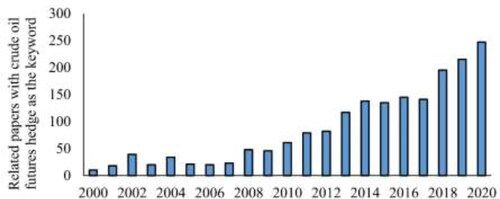
It can be seen in Figure 1 that the number of the research on crude oil futures hedging is increasing year by year. Crude oil futures hedging has become a practical common concern problem in the industry and academia. Through combing these retrieved literature, we find that many of them study the methods to decide OHR, wherein the routine is to model volatilities of spot and futures returns. There are two main methods for modeling and forecasting in the volatilities of crude oil prices. The first approach adopts popular GARCH-type models, such as Wang et al. (2019), Chun et al. (2019), Okorie and Lin (2020). The second approach is the Markov regime-switching model and its improved models (Alizadeh et al., 2008). The assumption of volatility models mentioned above is that the residuals obey a normal or Student-t distribution, few studies provide theoretical and empirical results considering the effect of skewness on OHR.

With the deepening of understanding of financial market, academics see more value of skewness in financial issue research. Skewness means fat tail and asymmetry in asset returns (Adcock et al., 2015). Compared to positive skewness, it seems that we are caring more about the negative skewness, which scales to the possibility at which extremes occur, just like the black swan event in stock market, unpredictable and devastating. In the classical financial theories, the proposal of Capital Asset Pricing Model (Sharpe, 1964) provided a new guideline to identify risks and price asset, while its basic assumption is that returns follow the normal distribution, which neglects the influence of extreme loss, so the skewness, as a proxy for tail risk, gets more and more attention and has been extensively applied in financial issue research afterwards. For example, Kraus and Litzenberger (1976) developed the CAPM model with the skewness incorporated. Adcock (2010) proposed a general multivariate model, incorporating both skewness and kurtosis, based on the multivariate extended skew-Student-t distribution, to investigate asset pricing and portfolio selection issue. Eling (2012) confirmed that the skew-normal distribution was a better alternative for modeling capital market returns compared to the normal distribution. Carmichael and Coën (2013) derived explicit expressions of assets skewness premiums and studied the effect of skewness and coskewness on asset valuation. Bernardi (2013) provided an analytical formula for some well-known risk measures based on finite mixtures of univariate skewed normal. Other skewness relevant papers can be found in Mills (1995), Harvey and Siddique (2000), Bauwens and Laurent (2005), Vernic (2006), Beranger et al. (2019).

In spite of the extensive discussion of skewness in the field of finance, however, for the risk management, especially for the case with futures hedging, existing research is not enough. Harvey et al. (2004) applied the Bayesian approach to skew-normal distribution to determine the optimal portfolio within a family of linear utility functions. Benedetti (2004) adopted both skew-normal and skew-t distributions to construct the optimal hedge fund portfolios. Although the literature mentioned above has analyzed the influence of skewness, it involves some unreasonable assumptions. Lien (2010) looked into the effect of skewness on production and hedging decision, not accounting for the basis risk between spot and futures. Barbi and Romagnoli (2018) checked out the effect of skewness on optimal futures demand, but solely used a standard constant relative risk aversion utility function. In order to further investigate the effect of skewness on futures hedging and cover the shortage of existing research, this paper assumes that the return of the hedged portfolio follows a skew-normal distribution, adopts Variance, VaR and CVaR as risk measures, incorporates the futures basis, and analyzes how the skewness and its changes influence the optimal hedging decisions through empirical test based on the crude oil data.

3. The skew-normal distribution

The Skew-normal distribution has been introduced by Azzalini (1985), which extends the normal distribution by introducing a parameter to express skewness. Suppose X is a random variable with a standard skew-normal distribution, we denote it by $X\sim SN(0,1;\lambda ).$ Here, $\lambda$ is the shape parameter, also measures the skewness. The probability density function of a standard skew-normal distribution is: (1) $$f\left(x\right)=2\varphi \left(x\right)\mathrm{\Phi }\left(\lambda x\right)$$(1) where $\varphi (·)$ and $\mathrm{\Phi }(·)$ are the probability density function and cumulative distribution function for the standard normal distribution, respectively. Negative skewness means $\lambda$ is negative, while a positive skewness means a positive $\lambda .$ When $\lambda =0,$ a standard skew-normal distribution degrades into a standard normal distribution. Thus, the standard skew-normal distribution generalizes the standard normal distribution. Furthermore, we can introduce a general skew-normal distribution via a linear transformation as follows.

If $X\sim SN(0,1;\lambda ),$ and (2) $$Y=\xi +\omega X$$(2) then $Y$ obeys a skew-normal distribution, i.e. $Y\sim SN(\xi ,{\omega }^2,\lambda ).$ Here, $\xi$ and $\omega$ are location and scale parameters, respectively.

The most general theoretical results on the subjective characterization of risk measures are VaR and CVaR, which can be expressed as the function of quantile. If we assume the hedged portfolio return has a skew-normal distribution, the key step of calculating the risks is to obtain the α-quantile of the hedged portfolio return. However, it is difficult to find the expression of the α-quantile of a skew-normal distribution. Fortunately, Fung and Seneta (2016) provides the following approximate α-quantile function $F^{-1}(\alpha )$ of a standard skew-normal distribution. (3) $$F^{-1}\left(\alpha \right)=\{\begin{array}{c}-\sqrt{-\frac{2}{1+{\lambda }^2}ln(-2\mathit{\text{πλαln}}(2\pi \lambda \alpha \left)\right)},\mathit{\text{if λ}}>0\\ -\sqrt{-2ln\left(\frac{\alpha }{2}\sqrt{-4\pi ln\left(\frac{\alpha }{2}\sqrt{2\pi }\right)}\right)},\mathit{\text{if λ}}<0\end{array}\mathrm{}as\mathrm{}\alpha \to 0^{+}$$(3)

Since $\alpha$ is assumed to be 0.01, 0.025 or 0.05, which are closed to 0, Eq.3(3) $$F^{-1}\left(\alpha \right)=\{\begin{array}{c}-\sqrt{-\frac{2}{1+{\lambda }^2}ln(-2\mathit{\text{πλαln}}(2\pi \lambda \alpha \left)\right)},\mathit{\text{if λ}}>0\\ -\sqrt{-2ln\left(\frac{\alpha }{2}\sqrt{-4\pi ln\left(\frac{\alpha }{2}\sqrt{2\pi }\right)}\right)},\mathit{\text{if λ}}<0\end{array}\mathrm{}as\mathrm{}\alpha \to 0^{+}$$(3) is applicable for calculating the values of VaR and CVaR with the transformation of $F_y^{-1}(\alpha )=F^{-1}(\alpha )\omega +\xi .$

4. Futures hedging frameworks

Hedging risk is the main function of futures. We suppose that an investor uses crude oil futures to avoid the price risk of crude oil spot. Then we can propose a hedged portfolio including one unit of underlying asset in long position and a certain amount of futures in short position. Let $\widetilde{r_p},$ $\widetilde{r_s}$ and $\widetilde{r_f}$ be the random returns of the hedged portfolio, spot commodity, futures commodity respectively. Denote $h$ be the hedge ratio, then the return of the hedged portfolio can be expressed by (4) $$\widetilde{r_p}=\widetilde{r_s}-h\widetilde{r_f}$$(4)

In this paper, we assume that $\widetilde{r_p}$ follows a skew-normal distribution, i.e., $\widetilde{r_p}\mathrm{}˜SN(\xi ,\omega ;\lambda ).$ Given a futures position of $h,$ we utilize the maximum likelihood estimation (MLE) method to estimate the parameters $\xi ,$ $\omega$ and $\lambda$ of $\widetilde{r_p}.$ Note that MLE can be implemented by the SN.mle package in R software. Therefore, we don’t intend to present the tedious theoretical formula of MLE method.

4.1. The minimum-variance hedging framework

Ederington (1979) derived the optimal hedge ratio based on minimum-variance hedging, wherein the optimal hedging ratio is decided by minimizing the variance of $\widetilde{r_p}.$ According to Eq.(4)(4) $$\widetilde{r_p}=\widetilde{r_s}-h\widetilde{r_f}$$(4) , the variance of the hedged portfolio return is (5) $${\sigma }_p^2={\sigma }_s^2+h^2{\sigma }_f^2-2h\rho {\sigma }_s{\sigma }_f$$(5) where ${\sigma }_{sf}$ denotes the covariance of $\widetilde{r_s}$ and $\widetilde{r_f}$ with correlation coefficient of $\rho .$ ${\sigma }_s$ and ${\sigma }_f$ are the standard deviations of the spot and futures returns, respectively. Then, we can obtain the optimal hedge ratio by solving the unconstrained model of ${\mathit{min}}_h{\sigma }_p^2.$ (6) $$h_{MV}^{\mathrm{*}}=\rho \frac{{\sigma }_s}{{\sigma }_f}$$(6)

4.2. The minimum-VaR hedging framework

When considering unilateral risk or extreme risk, variance is no longer an appropriate measure of risk since it equates gains with losses. This has led to the emergence of alternative measures of risk. Of these, perhaps the most widely used is Value at Risk (VaR). Value-at-Risk (VaR) is a candidate risk measure, which is defined as a potential amount of loss on a portfolio with a given probability over a certain period. As shown in the previous literature, some researchers have studied the hedging strategies for risk control of energy price based on minimum-VaR hedging (see Youssef et al., 2015). Under the skew-normal distribution of the hedged portfolio return in this paper, we provide the risk measure of VaR as follows.

Proposition 1.

Assume that the return of the hedged portfolio has a skew-normal distribution, $\widetilde{r_p}˜SN(\xi ,{\omega }^2;\lambda ),$ then the risk of the hedged portfolio return measured by VaR is (7) $$\mathit{VaR}=-F^{-1}\left(\alpha \right)\omega -\xi$$(7)

And the optimal hedge ratio minimizing VaR solves the following first-order condition of (8) $${\frac{\partial \mathit{VaR}}{\partial h}|}_{h=h_{\mathit{VaR}}^{\mathrm{*}}}=0$$(8) where $F^{-1}(\alpha )$ is the α − quantile of the standard skew-normal distribution, which is calculated from Eq.3(3) $$F^{-1}\left(\alpha \right)=\{\begin{array}{c}-\sqrt{-\frac{2}{1+{\lambda }^2}ln(-2\mathit{\text{πλαln}}(2\pi \lambda \alpha \left)\right)},\mathit{\text{if λ}}>0\\ -\sqrt{-2ln\left(\frac{\alpha }{2}\sqrt{-4\pi ln\left(\frac{\alpha }{2}\sqrt{2\pi }\right)}\right)},\mathit{\text{if λ}}<0\end{array}\mathrm{}as\mathrm{}\alpha \to 0^{+}$$(3)

4.3. The minimum-CVaR hedging framework

Although VaR is widely used in risk management, it is not a “coherent” measure and fails to satisfy the “subadditivity” property (Artzner et al., 1999). Besides, VaR cannot capture the extreme losses that are greater than the threshold amount (Rockafellar & Uryasev, 2002). Conditional Value-at-Risk (CVaR) is another tool for risk measuring, which provides the tail information of loss and is favorable to keeping away the extreme finance risk with very small probability. In the context of futures hedging, Harris and Shen (2006) estimated minimum-VaR and minimum-CVaR hedge ratios nonparametrically using historical simulation data. Roustai et al. (2018) applied CVaR to quantify the loss in energy markets recently. We also provide the CVaR of the hedged portfolio return in the following Proposition.

Proposition 2.

Assume that the hedged portfolio return has a skew-normal distribution, $\widetilde{r_p}˜SN(\xi ,\omega ;\lambda ),$ then the risk of $\widetilde{r_p}$ measured by CVaR is (9) $$\mathit{CVaR}=-\omega k_{\alpha }-\xi$$(9) where $k_{\alpha }=\frac{{\int }_{-\mathrm{\infty }}^{F^{-1}(\alpha )}xf(x)dx}{\alpha },$ $f(·)$ is the probability density function of a standard skew-normal distribution. $F^{-1}(\alpha )$ is the α − quantile of the standard skew-normal distribution, which is calculated from Eq.3(3) $$F^{-1}\left(\alpha \right)=\{\begin{array}{c}-\sqrt{-\frac{2}{1+{\lambda }^2}ln(-2\mathit{\text{πλαln}}(2\pi \lambda \alpha \left)\right)},\mathit{\text{if λ}}>0\\ -\sqrt{-2ln\left(\frac{\alpha }{2}\sqrt{-4\pi ln\left(\frac{\alpha }{2}\sqrt{2\pi }\right)}\right)},\mathit{\text{if λ}}<0\end{array}\mathrm{}as\mathrm{}\alpha \to 0^{+}$$(3) .

In order to solve the tedious integral, we derive the analytical expression of $k_{\alpha }$ based on Eq.1(1) $$f\left(x\right)=2\varphi \left(x\right)\mathrm{\Phi }\left(\lambda x\right)$$(1) . Thus, the explicit formula of CVaR is shown by (10) $$\mathit{CVaR}=-\omega k_{\alpha }-\xi \mathrm{}=-\frac{2\omega }{\alpha }{\int }_{-\mathrm{\infty }}^{F^{-1}\left(\alpha \right)}y\varphi \left(y\right)\mathrm{\Phi }\left(\lambda y\right)dy$$(10) $$\mathrm{}=-\frac{2\omega }{\alpha }\left[\frac{-1}{\sqrt{2\pi }}{e}^{-\frac{1}{2}{\left(F^{-1}\right(\alpha \left)\right)}^2}\mathrm{\Phi }\right(\lambda F^{-1}\left(\alpha \right))+\frac{\lambda }{\sqrt{2\pi (2+{\lambda }^2)}}\mathrm{\Phi }(\sqrt{1+{\lambda }^2}{F}^{-1}\left(\alpha \right)\left)\right]$$

Similarly, we can obtain the optimal hedge ratio $h_{\mathit{CVaR}}^{\mathrm{*}}$ by minimizing CVaR in Eq.10(10) $$\mathit{CVaR}=-\omega k_{\alpha }-\xi \mathrm{}=-\frac{2\omega }{\alpha }{\int }_{-\mathrm{\infty }}^{F^{-1}\left(\alpha \right)}y\varphi \left(y\right)\mathrm{\Phi }\left(\lambda y\right)dy$$(10) .

4.4. Hedge effectiveness

In order to effectively compare the hedging performance under the distribution assumption of normal or skew-normal, it needs to select appropriate evaluation criteria. There are some criteria for evaluating hedging performance, wherein the most widely used criteria is hedging effectiveness (Castelino, 1992; Ederington, 1979), which is shown by (11) $$HE=1-\frac{{\rho }_{\mathit{hedged}}}{{\rho }_{\mathit{unhedged}}}$$(11) where ${\rho }_{\mathit{hedged}}$ and ${\rho }_{\mathit{unhedged}}$ denote the risks of the hedged portfolio and unhedged portfolio returns, respectively. In this paper, the risks are Variance, VaR and CVaR. The larger HE is, the more effective the hedging model is.

5. Empirical analysis

There are many factors affect the globalized oil markets, such as the demand and supply for crude oil, economic and political disputes, and outbreak of events, these factors make the crude oil be suffered from large price shocks. Crude oil prices affect life, production, social stability, and so on. From a practical perspective, it is crucial to hedge the crude oil price risk especially in periods of dramatic price change. In empirical study, we investigate the performance of crude oil hedge portfolios when crude oil market’s skewness exists.

5.1. Data

In this part, we evaluate the risk and calculate the optimal hedge ratio based on the proposed models. To begin with, we collect price data (denominated in US dollars) of crude oil spot commodity and futures contracts from the two major worldwide crude oil markets of WTI and Brent. The closing prices of 759 trading days are from June 11, 2018 through May 19, 2021. The first time interval is from June 11, 2018 to March 19, 2019, used for in-sample testing, and the remaining is left for evaluating out-of-sample hedging performances by rolling window method with window width 200. All price data are collected from the wind database. Since the price of crude oil futures appears to be negative in the time interval, we define the returns $r_t$ as the following equation: (12) $$r_t=\frac{p_t-p_{t-1}}{p_{t-1}}$$(12) where $p_t$ is the value of the prices of crude oil spot and futures at time $t.$

Figures 2 and 3 present the prices and returns of Brent crude oil and WTI crude oil. It is easy to see that the trend of Brent crude oil spot and futures prices is basically the same. However, WTI crude oil futures has a remarkable basis due to the negative price in April 2020. We can also see that oil prices in the two crude oil markets fluctuates fiercely. Some outbreak events such as Sino-US trade war and COVID-19 may cause crashes in oil prices. The significant volatility of crude oil returns can also be seen in Figure 3.

Figure 2. Prices of Brent and WTI crude oil.

Source: Wind database.

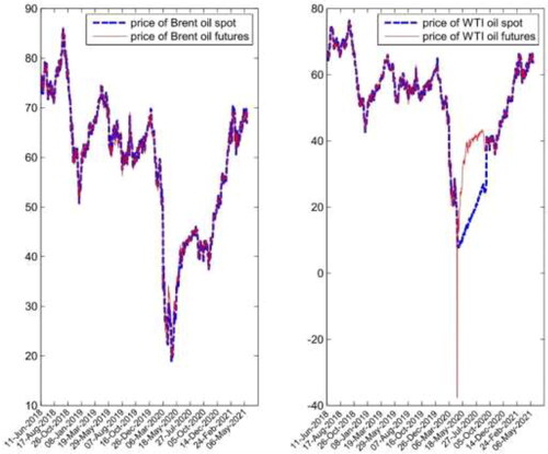
Figure 3. Returns of Brent and WTI crude oil.

Source: Wind database.

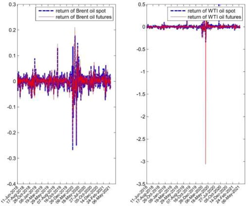
In Table 1, we provide the summary statistics of returns series for Brent and WTI crude oil. The largest unconditional mean returns are 0.0686% and −0.4244% for spot and futures data, respectively. In general, unconditional mean returns for the two crude oil investigated are small. Among all commodities considered, WTI futures appears to have the highest unconditional volatility of 1.5949% and Brent crude oil spot has the lowest unconditional volatility of 0.0888%. According to the skewness and leptokurtosis, unconditional distributions of spot and futures returns for the two crude oil are asymmetric, fat-tailed, and non-Gaussian.

Table 1. Descriptive statistics of spot and futures.

	WTI Spot Return	WTI Futures Return	Brent Spot Return	Brent Futures Return
Mean	0.000686	−0.004224	0.000283	0.000284
Min	−0.341410	−3.059700	−0.268700	−0.244040
Max	0.497090	0.376620	0.176810	0.210190
Var	0.001443	0.015949	0.000888	0.000912
Std	0.037992	0.126290	0.029791	0.030193
Skew	0.931990	−19.948500	−1.081700	−0.619280
Kurt	58.991800	465.965500	22.603300	19.764100
Corr	0.588760		0.937320

Source: Wind database.

To further test the normality of the returns, we present the Q-Q plots of Brent and WTI crude oil returns in Figure 4.

Figure 4. Q-Q plots of Brent and WTI crude oil returns.

Source: Wind database.

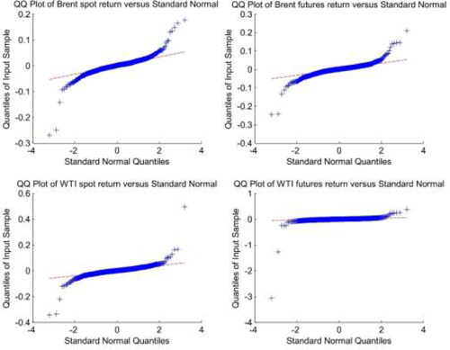
Figure 4 exhibits Q-Q plots for the spot and futures returns of WTI and Brent crude oil. We can see that many dots are located on or near the straight line with some of the other dots lying far away from the line, which results in the non-normality for returns of spot and futures. These characteristics make the skew-normal distribution a suitable distribution for the crude oil data since it accounts for both skewness and kurtosis. And then we apply the Jarque and Bera (1987) test statistic to test the partial normality of our data sets as our frames of reference are based on the shape of the distribution. Here, JBtest is proposed to test whether the sample data is normally distributed.

We can see from Table 2, none of the indices are well described under the hypothesis of normal distribution and the test rejected all H0 of normal distribution at a very high confidence level. Therefore, the returns of WTI and Brent are not normally distributed.

Table 2. Results of JBtest.

	H	P	JBSTAT	CV
WTI Return of Spot	1	1.0000e-03	99256.9485	5.9048
WTI Return of Futures	1	1.0000e-03	6828750.2962	5.9048
Brent Return of Spot	1	1.0000e-03	12301.2150	5.9048
Brent Return of Futures	1	1.0000e-03	8936.2103	5.9048

Source: Wind database.

5.2. Skewness test of the hedged portfolio

To further confirm the conclusion that crude oil futures and spot are skewed, we use the window sliding method to calculate the skewness of the hedged portfolio return shown in Figure 5, wherein the position of futures is fixed as 0.9, and the sliding window is 200 days.

Figure 5. Skewness of the crude oil hedged portfolio returns.

Source: Wind database.

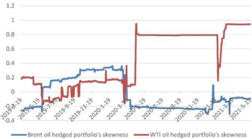
From Figure 5, we can find that the skewness of the Brent and WTI crude oil hedged portfolio return are not zero within 560 intervals of sliding test. It is widely known that the skewness of normal distribution is 0. That is, the returns series of the Brent and WTI crude oil hedged portfolio are not normally distributed. In particular, in April 2020 after the global outbreak of COVID-19, the skewness of the crude oil hedged portfolio returns increases significantly. This reflects the significance of this paper to study the influence of skewness on hedging decision. As stated in the introduction, the skewness of asset returns is usually remarkable under the extreme market.

According to Eqs.7(7) $$\mathit{VaR}=-F^{-1}\left(\alpha \right)\omega -\xi$$(7) and 9(9) $$\mathit{CVaR}=-\omega k_{\alpha }-\xi$$(9) , we can see that the hedge ratio minimizing the specific risk is closely related to the parameters of skew-normal distribution. From a forward direction, the return of the hedged portfolio $\widetilde{r_p}$ is different with different position of $h,$ which leads to different parameters in the distribution of $\widetilde{r_p}.$ In other words, parameters of the distribution and the position of futures are interactive. Figure 6 presents the relations between distribution parameters and the futures position $h.$

Figure 6. The effects of the hedge ratio on the distribution parameters.

Source: Wind database.

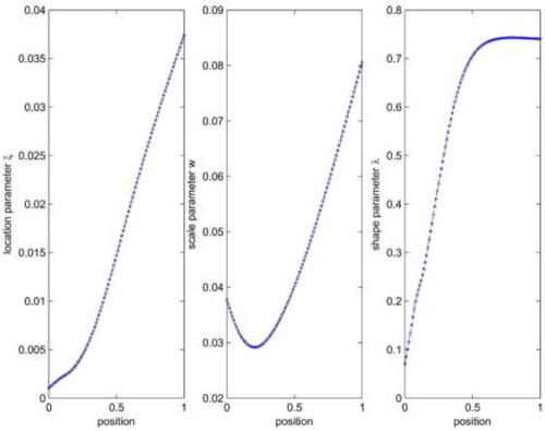
As can be seen from Figure 6, the distribution parameters of the hedged portfolio are dependent with the futures position $h.$ Therefore, we cannot provide the explicit formulas of the optimal hedge ratio that minimizing the risk expressed by Eqs.7(7) $$\mathit{VaR}=-F^{-1}\left(\alpha \right)\omega -\xi$$(7) and 9(9) $$\mathit{CVaR}=-\omega k_{\alpha }-\xi$$(9) . While, we can employ the traversal algorithm of position to obtain the optimal ratio in this paper.

5.3. The effect of skewness on hedging

In order to illustrate the effect of considering skewness on risk identification and hedging strategy, a hedging performance comparison between normal assumption and skewed normal assumption is conducted. Using the same sample data, the optimal hedge ratios are calculated using rolling windows method. Specifically, the sample returns data are divided into two segments: The first 200 observations are used for modelling, and the subsequent 560 observations to make the comparison.

At first, we want to confirm, even if the hedging position is not optimal, that’s to say, a series of possible hedging positions are incorporated into the hedging strategies, the risks after hedging based on the skewed normal distribution are smaller than that based on the normal distribution. The figures below show the simulation results that portfolio risk corresponding to different hedging ratios.

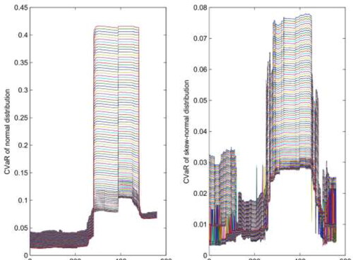
In order to save space, only results of adopting CVaR are showed here, results based on other risk measures are similar. From Figure 7, the maximum value of risks after hedging under the frame of skewed normal approximate 0.08 while the maximum for normal distribution reaches 0.1, and all the risk values within skewed normal distribution are slightly smaller than that within normal distribution. This sort of law can be seen clearly in Figure 8. In the results of adopting WTI crude oil data, risks after hedging based on the skewed normal distribution are considerably lower than that based on normal distribution. Conclusions can be drawn from aforementioned results that, whatever hedging strategies are adopted, skewed normal distribution enables us to identify risk fully and reduce it to the lowest.

Figure 7. CVaR of Brent crude oil hedged portfolio with different positions.

Source: Wind database.

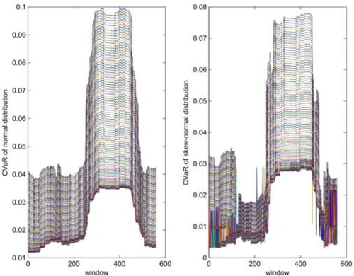
Figure 8. CVaR of WTI crude oil hedged portfolio with different positions.

Source: Wind database.

Following numerical simulation, we conduct an empirical analysis through real data, including in-sample and out-of-sample tests, the former means using optimal hedging ratios of current period to hedging current risk while the latter means using current optimal hedging ratios to hedging the risk of next period. For the in-sample test, we first calculate optimal hedging positions by means of rolling window method, then get a series of returns of portfolios by incorporating optimal positions, finally calculate risks of these portfolio returns, which are represented in Tables 3 and 4.

Table 3. variance and VaR of the hedged portfolio with Brent oil futures.

$\alpha$	Unhedged variance	Normal variance	Normal efficiency	skew-normal variance	skew-normal efficiency
0.01	0.00106804	0.00014093	0.8680	0.00013873	0.8701
0.025	0.00106804	0.00014132	0.8677	0.00013935	0.8695
0.05	0.00106804	0.00014097	0.8680	0.00013964	0.8693
$\alpha$	Unhedged VaR	Normal VaR	normal efficiency	skew-normal VaR	skew-normal efficiency
0.01	0.08310697	0.03545438	0.5734	0.03249129	0.6090
0.025	0.06158675	0.02236547	0.6368	0.02221084	0.6394
0.05	0.04033000	0.01452311	0.6399	0.01448651	0.6408

Source: Wind database.

Table 4. variance and VaR of the hedged portfolio with WTI oil futures.

$\alpha$	Unhedged variance	Normal variance	Normal efficiency	skew-normal variance	skew-normal efficiency
0.01	0.00180836	0.01325607	−6.3304	0.00823415	−3.5534
0.025	0.00180836	0.01352966	−6.4817	0.00845996	−3.6783
0.05	0.00180836	0.01356996	−6.5040	0.00845907	−3.6778
$\alpha$	Unhedged VaR	Norma VaR	normal efficiency	skew-normal VaR	skew-normal efficiency
0.01	0.10969608	0.08227521	0.0489	0.04887263	0.5545
0.025	0.06889837	0.03658715	0.0315	0.03151173	0.5426
0.05	0.04634164	0.01898693	0.0235	0.02348099	0.4933

Source: Wind database.

Tables 3 and 4 show that, for Brent crude oil, whether it is based on the minimum variance strategy or the minimum VaR strategy, the hedging portfolios obtained under the normal assumption and the skewed normal assumption can significantly reduce the risk of the spot. The efficiency of the strategy based on the minimum variance target is 86%, the efficiency of the strategy based on the minimum VaR target is slightly lower, but both exceed 60%, indicating that both strategies can effectively avoid the risk of spot price fluctuations. But for WTI crude oil, the effects of the two strategies are not very satisfactory: the risk aversion of the strategy with VaR as the risk measurement is less than 60%, and the strategy with the variance as the risk measurement may even increase the risk of volatility. The most important point is that, for all the crude oil varieties and risk measures, the hedging efficiency under the framework of skewed normal distribution is always better than that of normal distribution, especially for WTI crude oil with VaR as risk measure. This further illustrates that the skewness of asset portfolio in hedging cannot be ignored.

The out-of-sample test results are showed in Figures 9–11. Here we first calculate optimal hedging ratios through rolling window method, then hedge the risk using optimal hedging ratios, so the figures show the risks after hedging based on different risk measures. Only results of Brent crude oil are showed for the sake of saving space. The confidence level is assumed to be 0.05 and the abscissa represents the scrolling inspection window.

Figure 9. variance of Brent crude oil hedged portfolio.

Source: Wind database.

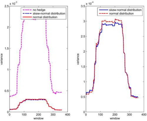
Figure 10. VaR of Brent crude oil hedged portfolio.

Source: Wind database.

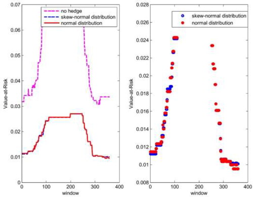
Figure 11. CVaR of Brent crude oil hedged portfolio.

Source: Wind database.

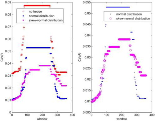
From Figures 9–11, we can see clearly how effective the hedging strategy obtained by the two hypotheses under each risk measure is. On the whole, the risk of each hedging portfolio is significantly lower than that of the spot. Through the right figures above, it is more convenient to compare strategies based on skew-normal distribution and normal distribution. At first, no single strategy, based on normal distribution or skewed normal distribution, has been shown to be absolutely superior, but most of the time the risk of the hedging portfolio under the skew-normal assumption is less than the normal assumption. In addition, under the three risk measures, the risk gap between strategies, considering skewness or not considering skewness, is different. The biggest gap appears in the case of CVaR while the gap of using VaR as risk measure is the smallest. Relatively speaking, when CVaR as the risk measure, neglect of skewness would cause greater bias, so skewness deserves more attention.

6. Conclusion

In this work we have investigated the effect of skewness on hedging decisions and hedging performance. We have used the skew-normal distribution to perform this task. The rationale behind the use of skew-normal distribution stems from the fact that it provides very good estimates for the crude oil data with highly asymmetric behavior and consequently with large skewness values. Some main valuable conclusions are soundly drawn.

Negative skewness exists in real-world hedged portfolios of crude oil generally, that’s to say, the possibility at which losses or extreme losses occur may be bigger than we think, and they deserve our attention. The results suggested that, skewness has a substantial impact on hedging decisions. Especially, when impacted by extreme events, the influence of skewness on decision-making cannot be ignored. The hedging strategy that ignores skewness is questioned because the hedging effect based on normal distribution assumption is not as good as that under skew-normal distribution assumption. Based on the conclusions in this paper, we can see, skewness is a considerable factor for micro-financial market research, and extreme risks should be accounted by every investor or producer. Although price fluctuations and extremes are likely to appear in most of commodities and assets, risks faced by crude oil may be the biggest, because crude oil is not only a commodity but a strategic military material. In addition, since prices of some products, like crude oil, are easy to be influenced by international political situation and present some kind of periodical characteristics, so how to identify the periods or states hidden behind and make accurate hedging decisions will be an interesting research direction.

Disclosure statement

No potential conflict of interest was reported by the authors.

Additional information

Funding

This paper is supported by Funds for International Cooperation and Exchange of the National Natural Science Foundation of China (71720107002); National Natural Science Foundation of China (No.71501076); Natural Science Fund of Guangdong (No.2014A030310454); Financial Service Innovation and Risk Management Research Base of Guangzhou; The Raising initial capital for High-level Talents of Central China Normal University (30101190001); Fundamental Research Funds for the Central Universities (CCNU19A06043, CCNU19TD006, CCNU19TS062); Humanities and Social Science Planning Fund from Ministry of Education (Grant No.21YJC790148).

References

- Abadie, L. M., Goicoechea, N., & Galarraga, I. (2017). Carbon risk and optimal retrofitting in cement plants: an application of stochastic modelling, Monte Carlo simulation and real options analysis. Journal of Cleaner Production, 142(1), 3117–3130. https://doi.org/10.1016/j.jclepro.2016.10.155
- Adcock, C. J. (2010). Asset pricing and portfolio selection based on the multivariate extended skew-Student-t distribution. Annals of Operations Research, 176(1), 221–234. https://doi.org/10.1007/s10479-009-0586-4
- Adcock, C., Eling, M., & Loperfido, N. (2015). Skewed distributions in finance and actuarial science: a review. The European Journal of Finance, 21(13–14), 1253–1281. https://doi.org/10.1080/1351847X.2012.720269
- Alizadeh, A. H., Alizadeh, N. K., & Pouliasis, P. K. (2008). A Markov regime switching approach for hedging energy commodities. Journal of Banking & Finance, 32 (9), 1970–1983. https://doi.org/10.1016/j.jbankfin.2007.12.020
- Artzner, P., Eber, F., Eber, J. M., & Heath, D. (1999). Coherent measures of risk. Mathematical Finance, 9(3), 203–228. https://doi.org/10.1111/1467-9965.00068
- Azzalini, A. (1985). A class of distribution which includes the normal ones. Scandinavian Journal of Statistic, 12, 171–178.
- Barañano, A., De La Peña, J. I., & Moreno, R. (2020). Valuation of real-estate losses via Monte Carlo simulation. Economic Research-Ekonomska Istraživanja, 33(1), 1867–1888. https://doi.org/10.1080/1331677X.2020.1756372
- Barbi, M., & Romagnoli, S. (2018). Skewness, basis risk, and optimal futures demand. International Review of Economics & Finance, 58(11), 14–29. https://doi.org/10.1016/j.iref.2018.02.021
- Bauwens, L., & Laurent, S. (2005). A new class of multivariate skew densities, with application to generalized autoregressive conditional heteroscedasticity models. Journal of Business & Economic Statistics, 23(3), 346–354. https://doi.org/10.1198/073500104000000523
- Benedetti, S. M. (2004). Hedge fund portfolio selection with higher moments [Master thesis]. University of Zurich.
- Beranger, B., Padoan, S. A., Xu, Y., & Sisson, S. A. (2019). Extremal properties of the univariate extended skew-normal distribution. Statistics & Probability Letters, 147, 73–82. https://doi.org/10.1016/j.spl.2018.09.018
- Bernardi, M. (2013). Risk measures for skew normal mixtures. Statistics & Probability Letters, 83(8), 1819–1824. https://doi.org/10.1016/j.spl.2013.04.016
- Bhutto, S. A., Ahmed, R. R., Streimikiene, D., Shaikh, S., & Streimikis, J. (2020). Portfolio investment diversification at global stock market: A cointegration analysis of emerging BRICS(P) group. Acta Montanistica Slovaca, 25(1), 57–69.
- Carmichael, B., & Coën, A. (2013). Asset pricing with skewed-normal return. Finance Research Letters, 10(2), 50–57. https://doi.org/10.1016/j.frl.2013.01.001
- Castelino, M. G. (1992). Hedge effectiveness: Basis risk and minimum variance hedging. Journal of Futures Markets, 12(2), 187–201. https://doi.org/10.1002/fut.3990120207
- Chai, S. L., & Zhou, P. (2018). The Minimum-CVaR strategy with semi-parametric estimation in carbon market hedging problems. Energy Economics, 76, 64–75. https://doi.org/10.1016/j.eneco.2018.09.024
- Chun, D., Cho, H., & Kim, J. (2019). Crude oil price shocks and hedging performance: A comparison of volatility models. Energy Economics, 18(6), 1132–1147.
- Ederington, L. H. (1979). The hedging performance of the new futures markets. The Journal of Finance, 34(1), 157–170. https://doi.org/10.1111/j.1540-6261.1979.tb02077.x
- Eling, M. (2012). Fitting insurance claims to skewed distributions: are the skew-normal and skew-student good models? Insurance: Mathematics and Economics, 51(2), 239–248. https://doi.org/10.1016/j.insmatheco.2012.04.001
- Falkowski, M., Sierpińska-Sawicz, A., & Szczepankowski, P. (2020). The effectiveness of hedge fund investment strategies under various market conditions. Contemporary Economics, 14(2), 127–144. https://doi.org/10.5709/ce.1897-9254.336
- Feng, Z. H., Wei, Y. M., & Wang, K. (2012). Estimating risk for the carbon market via extreme value theory: an empirical analysis of the EU ETS. Applied Energy, 99, 97–108. https://doi.org/10.1016/j.apenergy.2012.01.070
- Fung, T., & Seneta, E. (2016). Tail asymptotics for the bivariate skew normal. Journal of Multivariate Analysis, 144, 129–138. https://doi.org/10.1016/j.jmva.2015.11.002
- Hamiton, J. D. (2009). Understanding crude oil prices. Energy, 30, 179–206.
- Harris, R. D. F., & Shen, J. (2006). Hedging and value at risk. Journal of Futures Markets, 26(4), 369–390. https://doi.org/10.1002/fut.20195
- Harvey, C. R., Liechty, M., Lietchy, W., & Muller, P. (2004). Portfolio selection with higher moments: A Bayesian decision theoretical approach (working paper). Duke University.
- Harvey, C. R., & Siddique, A. (2000). Conditional skewness in asset pricing tests. The Journal of Finance, 55(3), 1263–1295. https://doi.org/10.1111/0022-1082.00247
- Hemmati, R., Saboori, H., & Saboori, S. (2016). Stochastic risk-averse coordinated scheduling of grid integrated energy storage units in transmission constrained windthermal systems within a conditional value-at-risk framework. Energy, 113 (15), 762–775. https://doi.org/10.1016/j.energy.2016.07.089
- Jarque, C. M., & Bera, A. K. (1987). A test for normality of observations and regression residuals. International Statistical Review/Revue Internationale de Statistique, 55(2), 163–172. https://doi.org/10.2307/1403192
- Johnson, L. L. (1960). The theory of hedging and speculation in commodity futures. The Review of Economic Studies, 27(3), 139–151. https://doi.org/10.2307/2296076
- Kraus, A., & Litzenberger, R. H. (1976). Skewness preference and the valuation of risk assets. The Journal of Finance, 31(4), 1085–1100.
- Lien, D. (2010). The effects of skewness on optimal production and hedging decisions: An application of the skew-normal distribution. Journal of Futures Markets, 30(3), 278–289.
- Liu, B., Ji, Q., & Fan, Y. (2017). Dynamic return-volatility dependence and risk measure of CoVaR in the oil market: a time-varying mixed copula model. Energy Economics, 68, 53–65. https://doi.org/10.1016/j.eneco.2017.09.011
- Lu, Z. G., Qi, J. T., Wen, B., & Li, X. P. (2016). A dynamic model for generation expansion planning based on conditional value-at-risk theory under low-carbon economy. Electric Power Systems Research, 141, 363–371. https://doi.org/10.1016/j.epsr.2016.08.011
- Mills, T. C. (1995). Modelling skewness and Kurtosis in the London stock exchange Ft-Se index return distributions. Journal of the Royal Statistical Society, 44(3), 323–332.
- Myers, R. J., & Thompson, S. R. (1989). Generalized optimal hedge ratio estimation. American Journal of Agricultural Economics, 71(4), 858–867. https://doi.org/10.2307/1242663
- Naqvi, B., Mirza, N., Naqvi, W. A., & Rizvi, S. K. A. (2017). Portfolio optimization with higher moments of risk at the Pakistan Stock Exchange. Economic Research-Ekonomska Istraživanja ˇ, 30(1), 1594–1610. https://doi.org/10.1080/1331677X.2017.1340182
- Okorie, D. I., & Lin, B. (2020). Crude oil price and cryptocurrencies: Evidence of volatility connectedness and hedging strategy. Energy Economics, 87(3), 104703. https://doi.org/10.1016/j.eneco.2020.104703
- Reboredo, J. C., & Ugando, M. (2015). Downside risks in EU carbon and fossil fuel markets. Mathematics and Computers in Simulation, 111(5), 17–35. https://doi.org/10.1016/j.matcom.2014.12.001
- Rockafellar, R. T., & Uryasev, S. (2002). Conditional value-at-risk for general loss distributions. Journal of Banking & Finance, 26 (7), 1443–1471. https://doi.org/10.1016/S0378-4266(02)00271-6
- Roustai, M., Rayati, M., Sheikhi, A., & Ranjbar, A. (2018). A scenario-based optimization of smart energy hub operation in a stochastic environment using conditional-valueat-risk. Sustainable Cities and Society, 39(5), 309–316. https://doi.org/10.1016/j.scs.2018.01.045
- Segnon, M., Lux, T., & Gupta, R. (2017). Modeling and forecasting the volatility of carbon dioxide emission allowance prices: a review and comparison of modern volatility models. Renewable and Sustainable Energy Reviews, 69(3), 692–704. https://doi.org/10.1016/j.rser.2016.11.060
- Sharpe, W. E. (1964). Capital asset prices: A theory of market equilibrium under condition of risk. The Journal of Finance, 19(3), 425–442.
- Tekiner-Mogulkoc, H., Coit, D. W., & Felder, F. A. (2015). Mean-risk stochastic electricity generation expansion planning problems with demand uncertainties considering conditional value-at-risk and maximum regret as risk measures. International Journal of Electrical Power & Energy Systems, 73(12), 309–317. https://doi.org/10.1016/j.ijepes.2015.05.003
- Vernic, R. (2006). Multivariate skew-normal distributions with applications in insurance. Insurance: Mathematics and Economics, 38(2), 413–426. https://doi.org/10.1016/j.insmatheco.2005.11.001
- Wang, Y. D., Geng, Q. J., & Meng, F. Y. (2019). Futures hedging in crude oil markets: A comparison between minimum-variance and minimum-risk frameworks. Energy, 181, 815–826. https://doi.org/10.1016/j.energy.2019.05.226
- Youssef, M., Belkacem, L., & Mokni, K. (2015). Value-at-risk estimation of energy commodities: a long-memory GARCH-EVT approach. Energy Economics, 51, 99–110. https://doi.org/10.1016/j.eneco.2015.06.010
- Yu, W. H., Yang, K., Wei, Y., & Lei, L. K. (2018). Measuring Value-at-Risk and Expected Shortfall of crude oil portfolio using extreme value theory and vine copula. Physica A: Statistical Mechanics and Its Applications, 490(9), 1423–1433. https://doi.org/10.1016/j.physa.2017.08.064