A double interaction-based financing group decision-making framework considering uncertain information and inconsistent assessment

Abstract

Financing group decision-making (FGDM), which is an important stage of project financing, has unique characteristics: large investments and long payback horizons. Its evaluation results are likely to be distorted if we ignore the uncertain information and inconsistent assessment during the decision-making process. In this study, we propose a double interaction-based FGDM framework under uncertain information and inconsistent assessment. We modify the weight setting of evidence reasoning and aggregation method of probabilistic linguistic term sets to process the above two issues. The proposed framework is applied in a detailed case study analysis to display its effectiveness and stability. We expect the double interaction-based group decision-making framework under uncertain information and inconsistent assessment to be a useful tool to understand FGDM processes.

Keywords:

• Financing group decision-making
• uncertain information
• inconsistent assessment
• probabilistic linguistic term sets
• evidence reasoning
• double interaction

JEL CODES:

• B41
• C02
• D81
• G11

1. Introduction

Financing group decision-making (FGDM) refers to the important process of governments deciding to provide long-term funding, and plays a decisive role in large-scale projects, such as infrastructure development (Kissinger et al., 2019; Steffen, 2018). Understanding FGDM can directly and/or indirectly help governments to solve the funding problems of major projects (Chemmanur & John, 1996; Lamont, 1997), and thus deserves to be studied.

As an important stage of project financing, FGDM is a selection process that includes multiple factors (Tsai et al., 2013). Accordingly, it is also a complex multi-attribute group decision-making (MAGDM) problem. In contrast to general group decision-making problems, FGDM situations have unique characteristics, namely, they consider very large investments and long payback horizons. It is also almost impossible to change the financing scheme once it has been selected. Therefore, choosing a reasonable financing strategy is extremely important at the FGDM stage (Alavipour & Arditi, 2018).

This issue has both practical and theoretical significance. To investigate it, this study considers the following research question. What are the key factors while deciding? Different people have their own ideas. Past literature has identified the evaluation index system and applied it to the evaluation process (Chang, 2014; Grimsey & Lewis, 2002; Zhang, 2006). The consensus is that it is meaningful for decision makers to choose a reasonable evaluation index.

Other research has focused on information expression (Alonso, 2013; Gou et al., 2020; Sahi et al., 2013). Due to the incompleteness of information sets in real world decision situations, uncertainty often exists in the FGDM process (Jiang et al., 2005). To analyze this issue, Herrera et al. (1997) put forward linguistic information expression in group decision-making. Rodriguez et al. (2012) proposed to convert the natural language used in information evaluation into hesitant fuzzy linguistic term sets for analysis. In addition, Lourenzutti et al. (2017) proposed a language distribution assessment to express experts’ evaluations of an object, which requires experts to have a definite evaluation for the evaluation object. However, most evaluations are not entirely certain. Thus, Pang et al. (2016) proposed probabilistic linguistic term sets (PLTS), in which a set of linguistic terms and their corresponding probabilities are used to evaluate alternatives, and thereby, solve the complex problem of uncertain information. On this basis, Zhang et al. (2016) defined the distance measure of PLTS and studied its additive consistency, and Cheng et al. (2018) further combined PLTS and interactive technology to establish a risk investment evaluation model.

In addition to considering the evaluation index system and information expression, how to deal with uncertain information and aggregate the evaluated results are also important considerations in FGDM. The term “uncertain information” was defined by Zadeh (1965) to represent the uncertainties caused by the limited cognitive ability of human beings. It has a significant influence in decision-making processes (Liu et al., 2019; Tao et al., 2020). Some methods have been established to manage the effects of uncertain information on decision-making, such as probability theory, fuzzy sets, and evidence reasoning (ER). Among them, the ER theory is widely used because of its simplicity and the ease of dealing with multi-attribute decision analysis problems under uncertainty. The ER theory proposed by Yang and Xu (2002) and they distinguish indeterminate information, and ignorant information as distinct forms of uncertain information. This theory has a significant advantage regarding the fusion of multiple sources of information under uncertain information (Yang, 2001) and has been widely applied since it was proposed ( Chin et al., 2009; Kong et al., 2015; Tang et al., 2017; Wang, Kai, Guan, Yu, & Liu et al., 2019 ).

Additionally, the weighting assigned to different options in a decision, referred to as weight setting, has a significant influence on the decision result. Scholars have studied how decision-makers determine the relevant weights using the existing information in the decision-making process (Yuan et al., 2020). Specifically, the gray correlation helps study the problem of grey space, measuring the correlation between the reference sequence and the comparison sequence. Mao and Wu (2019) improved the gray correlation analysis approach by using probabilistic linguistic measurement distance to determine the corresponding attribute weights. Wang et al. (2019) used gray correlation analysis and the analysis hierarchy process to obtain the weight values of the indices. Yue (2017) developed an entropy-based approach to understand the weight setting process of experts in a group decision-making setting. Chang et al. (2013) proposed that the weights of options with high information consistency should be increased to prevent causing insufficient probabilities under uncertain information. Nonetheless, a research gap remains. In our framework, we propose the concept of “uncertainty degree” to investigate how uncertain information affects the weight setting process.

Another important issue is information aggregation. In recent years, some information aggregation approaches have been developed. Yang (2001) developed an ER algorithm, which is a flexible and useful mathematical tool for combining uncertain information sets. Pang et al. (2016) proposed the probabilistic linguistic weighted averaging (PLWA) operator based on the PLTS. However, in FGDM, each assessment of an expert’s decision-making process is carried out independently, which makes it difficult to draw a consistent conclusion using the above information aggregation method. Specifically, information interactions need to be considered.

Studies from the past few decades show that interactive decision-making with constant communication and interactions among evaluation experts means participants gradually and dynamically learn personal preference structures and thus, obtain the most satisfactory results (Bashiri & Badri, 2011; Han & Li, 1994; Reverberi & Talamo, 1999). To represent this, Han and Li (1994) proposed a simple calculation formula to evaluate the revised priority order. Lourenzutti et al. (2017) considered groups of decision makers with all their different opinions, heterogeneous types of information, criteria interaction, fuzzy measure identification and dynamic environments. Cheng at el. (2018) considered the consistency of assessing results and the weights of attributes through interactions among venture capital providers, and between venture capital providers and entrepreneurs. Chen and Zhang (2020) focused on the interaction among criteria in their methodology to deduce the weighting system. Among the existing approaches to information aggregation with interaction, most of the existing research focuses on interaction between experts. It lacks consideration of interaction between decision parameters. Different parameters may lead to different results. Decision makers must decide which parameters should be chosen to influence decisions and which results are credible without interaction.

The above literature review highlights several research gaps. (1) It is not clear how to process uncertain information using PLTS. This implies that for FGDM, how to set and adjust weights in an uncertain environment has not been well-studied. (2) In the information aggregation process, interactions between experts have been considered, but the interactions between parameters are rarely considered. Further, analysis of these two types of interaction under uncertain information at the same time are even more scarce.

To construct an effective method in FGDM and choose the most appropriate financing scheme, we propose a double interaction-based FGDM under uncertain information and inconsistent assessment. The highlights of our study can be summarized as follows: First, we propose a double interaction-based aggregation framework, which considers the consistency and similarity of the PLTS matrix together with gray correlation analysis under uncertain information and inconsistent assessment. Second, we use the modified ER and PLTS to process uncertain information, and provide evidence of their effectiveness. Third, different tools are applied in robustness tests to verify the validity of our framework.

The remainder of this study is organized as follows: In Section 2, we introduce the basic concepts of PLTS and ER. In Section 3, we propose a double interaction-based MAGDM method using the improved ER and PLTS under uncertain information and inconsistent assessment. In Section 4, the FGDM process is shown with the help of a case study and the validity of our framework is further verified. The final section presents the conclusions and future research directions.

2. Preliminaries

Here, we introduce some basic concepts and features of PLTS and ER and describe the process of interactive decision making.

2.1. Probabilistic linguistic term set

According to Pang et al. (2016), the PLTS formed by combining linguistic term sets and probability can be widely used. Thereby, the decision maker not only gives a language-based evaluation of a target object, but also supplies the probability information of the evaluation.

Definition 1

(Pang et al., 2016). Let $H=\left\{H_{\alpha }\right|\alpha =0,\mathrm{}1,\dots ,\tau \}$ be a linguistic term; then, a set of probabilistic linguistic terms$\mathrm{}S(p)$ is defined as follows: (1) $$S\left(p\right)=\left\{S^{\left(k\right)}\left(p^{\left(k\right)}\right)|S^{（k）}\in H,p^{\left(k\right)}\ge 0,\mathrm{k}=1,\mathrm{}2,\dots ,\#\mathrm{S}\left(\mathrm{p}\right),\sum _{k=1}^{\#\mathrm{S}\left(\mathrm{p}\right)}{\mathrm{p}}^{\left(k\right)}\le 1\right\},$$(1) where $S^{\left(k\right)}(p^{\left(k\right)})$ is the probability $p^{\left(k\right)}$ of the linguistic term $S^{\left(k\right)};\#\mathrm{S}(\mathrm{p})$ represents the number of different linguistic terms in $S(p).$

According to Pang et al. (2016), any two linguistic terms that belong to $H$ can be combined as follows: (2) $$S^{\left(k_i\right)}{p}^{\left(k_i\right)}\mathrm{*}{S}^{\left(k_i\right)}{p}^{\left(k_j\right)}=H_{p^{\left(k_i\right)}\mathrm{*}i+p^{\left(k_j\right)}\mathrm{*}j}.$$(2)

Definition 2

(Pang et al., 2016). Let $S_i(p)=\{S_i^{\left(k_i\right)}(p_i^{\left(k_i\right)})|k_i=1,\mathrm{}2,\dots ,\#{\mathrm{S}}_i(\mathrm{p})$}$\left(i=1,\mathrm{}2,\dots ,s\right)$ be the probabilistic linguistic term set; the corresponding weights are$\mathrm{}\omega =\{{\omega }_1,{\omega }_2,\dots ,{\omega }_s\}$ and they satisfy ${\omega }_iϵ[0,1]\mathrm{}$ and ${\sum }_{i=1}^s{\omega }_i=1.$ The PLWA operator is as follows: (3) $${\mathit{PLWA}}_{\omega }\left({\mathrm{S}}_1\left(\mathrm{p}\right),{\text{S}}_2\left(\mathrm{p}\right),\mathrm{\cdots },{\text{S}}_{\mathrm{s}}\left(\mathrm{p}\right)\right)\mathrm{}={\omega }_1{S}_1\left(p\right)+{\omega }_2{S}_2\left(p\right)+\cdots {\omega }_s{S}_s\left(p\right).$$(3)

Definition 3

(Pang et al., 2016). Let$\mathrm{}H=\left\{H_{\alpha }\right|\alpha =0,1,\dots ,\tau \}$ be a linguistic term; $S_1(p)=\{S_1^{\left(k_1\right)}(p_1^{\left(k_1\right)})|\mathrm{k}=1,\mathrm{}2,\dots ,\#{\mathrm{S}}_1(\mathrm{p})$} and $S_2(p)=\{S_2^{\left(k_2\right)}(p_2^{\left(k_2\right)})|\mathrm{k}=1,\mathrm{}2,\dots ,\#{\mathrm{S}}_2(\mathrm{p})$} are the sets of two probabilistic linguistic terms based on $S.$ $H_{\mathrm{\alpha }}^{(k_1)}$ and $H_{\mathrm{\alpha }}^{(k_2)}$are the linguistic terms corresponding to $S_1^{(k_1)}$ and $S_2^{(k_2)},$ respectively. Therefore, the distance between $S_1(p)$ and $S_2(p)$ is expressed as: (4) $$D\left(S_1\left(p\right),S_2\left(p\right)\right)=\sqrt{\frac{1}{\#{\mathrm{S}}_1\left(\mathrm{p}\right)\#{\mathrm{S}}_2\left(\mathrm{p}\right)}{\sum }_{k_1=1}^{\#{\mathrm{S}}_1\left(\mathrm{p}\right)}{\sum }_{k_2=1}^{\#{\mathrm{S}}_2(\mathrm{p}}{\left(\frac{H_{\mathrm{\alpha }}^{\left(k_1\right)}{p}_1^{\left(k_1\right)}-H_{\mathrm{\alpha }}^{\left(k_2\right)}{p}_2^{\left(k_2\right)}}{\tau }\right)}^2}.$$(4)

2.2. Evidence reasoning

ER is based on people’s understanding of objective existence. People use knowledge and clues to represent uncertain events using an uncertainty measurement method. This method is used in many uncertain multiple attribute decision-making problems.

For a specific decision-making problem, assume there are $L$ evaluation sets$\mathrm{}e=｛el｝,l＝1,\mathrm{}2,\dots ,L.$ The comprehensive attribute of evaluation is denoted by $y,$ which is determined by $T$ basic attributes and denoted by $e1,\mathrm{}e2,\dots ,\mathrm{}eT,$ respectively. The weights of the attributes $ei\left(i=1,\mathrm{}2,\dots ,T\right)\text{are represented by}Wi,$ $0\le Wi\le 1,$ and ${\sum }_{i=1}^T{w}_i=1.$ We use ${\beta }_{n,i}(a_l)$ to represent the basic attribute $ei$ of $a_l,$ which is the reliability of the evaluation level $Hn.$$\mathrm{}{\beta }_{H,i}(a_l)$ represents the reliability of the uncertain part of the basic attribute $ei$ of $a_l,$ with ${\beta }_{n,i}(a_l)\ge 0,{\sum }_{i=1}^N{\beta }_{n,i}(a_l)\le 1.$

In the evaluation of decision-making problems, any evaluation object can be expressed as follows: (5) $$S\left(a_i\right)=\left\{\left(e_{j,k},{\beta }_{j,k}\right);k=1,2,\dots ,T\right\},j=1,\mathrm{}2,\dots ,N.$$(5)

Among them, the research object has $T$ attributes, $e_{j,k}$ represents the attribute$\mathrm{}{e}_k,$ judged as$\mathrm{}{H}_j,$ and its reliability is ${\beta }_{j,k}.$ $w_k$ is set as the weight$\mathrm{}$ of the attribute $e_k.$ Then, the ER of $a_l$ is: (6) $$m_{j,k}=w_k{\beta }_{j,k},j=1,\mathrm{}2,\dots ,N$$(6) (7) $$m_{H,k}=1-\sum _{j=1}^N{m}_{j,k}=1-w_k\sum _{j=1}^N{\beta }_{j,k},$$(7) (8) $${\overline{m}}_{H,k}=1-w_k,{\tilde{m}}_{H,k}=w_i\left(1-\sum _{j=1}^N{\beta }_{j,k}\right).$$(8)

$m_{j,k}$ is the attribute $e_k$ of $a_l.$ When added to the weight index $w_k,$ it is judged as the basic reliability probability distribution of $H_n.$ ${\overline{m}}_{H,k}$ represents the basic belief probability that the weight-setting does not represent the real situation. ${\tilde{m}}_{H,k}$ is not a complete understanding of the problem at hand, as the real results may not follow a specific analysis framework.

Then, each attribute is a piece of evidence in the recursive orthogonal summation process, where the basic reliability probability of $k\mathrm{}+\mathrm{}1$ evidence fusion is obtained as: (9) $$m_{j,I(k+1)}=K_{I(k+1)}\left[m_{j,I\left(k\right)}{m}_{j,k+1}+m_{H,I\left(k\right)}{m}_{j,k+1}+m_{j,I\left(k\right)}{m}_{H,k+1}\right],$$(9) (10) $$m_{H,I(k+1)}=K_{I(k+1)}\left[{\tilde{m}}_{H,I\left(k\right)}{\tilde{m}}_{H,k+1}+{\overline{m}}_{H,I\left(k\right)}{\tilde{m}}_{H,k+1}+{\tilde{m}}_{H,I\left(k\right)}{\overline{m}}_{H,k+1}\right],$$(10) (11) $${\overline{m}}_{H,I(k+1)}=K_{I(k+1)}\left[{\overline{m}}_{H,I\left(k\right)}{\overline{m}}_{H,k+1)}\right],$$(11) (12) $$K_{I(k+1)}=\frac{1}{1-\sum _{j=1}^N\sum _{\begin{array}{c}i=1\\ i\ne j\end{array}}^N{m}_{j,I\left(k\right)}{m}_{i,k+1}}k=\left\{1,\mathrm{}2,\dots ,L-1\right\},$$(12) (13) $${\beta }_j=\frac{m_{j,I\left(L\right)}}{1-{\overline{m}}_{H,I\left(L\right)}},{\beta }_H=\frac{{\tilde{m}}_{H,I\left(L\right)}}{1-{\overline{m}}_{H,I\left(L\right)}}.$$(13)

Finally, we obtain graded evaluation results for decision-making problems.

3. Evaluation framework of financing group decision-making

The choice among financing alternatives is usually a MAGDM, which reflects the preference characteristics of financing decision-makers and the knowledge limitations of evaluation experts. To describe each option at the FGDM stage and fully consider the problems caused by uncertain information, this study presents a double interaction-based MAGDM method using improved ER and PLTSs, which can directly process uncertain information under multiple level evaluation. The inconsistent assessment problem under uncertain information is resolved by combining the double interaction and gray correlation analysis. The modified ER and PLTS are used to aggregate all information into a comprehensive result. Finally, we evaluate the alternatives for a final decision.

3.1. Expression of financing information

Here, financing plan research refers to the selection of a relatively optimal plan among the possible alternatives when there is a funding gap throughout the course of an engineering project.

First, the factors with significant influence on FGDM are determined. The existing research shows that financing is mainly affected by four types of comprehensive factors, namely financing economy, risk, feasibility, and reliability (Chang, 2014; Grimsey & Lewis, 2002; Zhang, 2006). Each of these factors is refined and decomposed into several basic factors. To analyze the financing plan, it is necessary to further evaluate the identified influencing factors.

For the project financing problem, we assume that there are $m$ alternatives, denoted as $A=\left\{a_{l}l=1,\mathrm{}2,\dots ,m\right\},$ and $N$ evaluation experts participate in the evaluation. The decision goal is composed of comprehensive attributes $y_i(i=1,\mathrm{}2,\dots ,\mathrm{t}),$ where $t$ indicates the number of comprehensive attributes. The comprehensive attributes $y_i(i=1,\mathrm{}2,\dots ,\mathrm{t})$ are composed of several basic attributes $e_j(j=n_{i-1}+1,\mathrm{}{n}_{i-1}+2,\dots ,n_i;i=1,\mathrm{}2,\dots ,\mathrm{t}),$ where $n_i-n_{i-1}$ indicates the number of basic attributes under each comprehensive attribute $y_i(i=1,\mathrm{}2,\dots ,\mathrm{t}).$ In addition, $n=n_t$ indicates the total number of basic attributes.

Generally, to facilitate the aggregation of basic attributes, we consider evaluating them using the same criteria they are associated with. At the same time, for data collection and collation, it is more natural to obtain evaluation information in a manner suitable to the specific attributes. That is, it is necessary to extract equivalent rules from the decision makers and then to convert the numerical information into equivalent expectations so that the quantitative and qualitative attributes can be considered simultaneously for analysis.

Experts usually evaluate qualitative evaluation indicators in the form of natural language. To make the evaluation information more convenient and intuitive, the corresponding evaluation levels can be used. These levels can be used to evaluate the overall situation of the financing scheme.

Additionally, it must be considered that an evaluation expert may not accurately determine the results at a specific evaluation level. Conversely, when evaluating qualitative basic attribute $e_j,$ several evaluation levels are considered. Each level is given a corresponding degree of belief according to the expert’s knowledge structure and experience level. Therefore, when $N\mathrm{}$ evaluation experts $V_q\left(q=1,\mathrm{}2,\dots ,N\right)$ participate in the decision-making process, for ${\forall a}_l\in A,$ the probabilistic linguistic evaluation of the alternative $a_l$ for the attribute $e_j$ under evaluation expert $V_q\left(q=1,\mathrm{}2,\dots ,N\right)$ can be represented as: (14) $$L_{lj}^{\mathrm{}q}\left(p\right)=\mathrm{}\left\{H_{\alpha },p_q^{\alpha ,j}\mathrm{}\alpha =1,\dots ,\mathrm{}\tau ;j=1,\mathrm{}2,\dots ,n;{\sum }_{\alpha =1}^{\mathrm{\tau }}{p}_q^{\alpha ,j}\le 1\right\}\left(q=1,\mathrm{}2,\dots ,N\right).$$(14)

Here, $\tau$ is the number of alternatives and $n$ is the number of evaluation attributes. This means that the evaluation expert $V_q$’s basic attribute $e_j$ of the alternative $a_l$ is evaluated as $H_{\alpha },$ with probability $p_q^{\alpha ,j}.$ The judgment matrix given is $p^{\left(q\right)\left(\delta \right)}\mathrm{}\left(q=1,\mathrm{}2,\dots ,N\right).$ $\delta$ is the number of judgment matrices given by the $q$ th evaluation expert ($\delta =1,2,\dots$). (15) $$p^{\left(q\right)\left(\delta \right)}=\left[\begin{array}{ccc}{S}_{11}^q\left(p\right)& \cdots & S_{1n}^q\left(p\right)\\ ⋮& \ddots & ⋮\\ S_{m1}^q\left(p\right)& \cdots & S_{mn}^q\left(p\right)\end{array}\right]$$(15)

Here, $S_{lj}^q\left(p\right)={\sum }_{\alpha =1}^{\tau }{p}_q^{\alpha ,j}*\alpha +\frac{{\sum }_{\alpha =1}^{\tau }\alpha }{\tau }*(1-{\sum }_{\alpha =1}^{\tau }{p}_q^{\alpha ,j})$ and this is referred to as the probabilistic linguistic term score. At the same time, $S_{lj}^q\left(p\right)$ is also an element of the judgment matrix $p^{\left(q\right)\left(\delta \right)}.$

3.2. Determination of weights under uncertain information

3.2.1. Experts’ weights

Reasonable and correct evaluations must fully consider the role that each evaluation expert plays. This requires financing decision-makers to attribute subjective weights according to the knowledge structures, experience levels, and personal preferences of evaluation experts. The subjective weights are given before the decision-making process is started and remain unchanged during this process. Another type of weight is the objective weight that evaluation experts use to express the information. The relevant combination of objective and subjective weights forms the final weight applied to the evaluation experts’ judgments. However, objective weights will dynamically modify the information expression according to conflicts in the decision-making process. In the proposed FGDM framework, assessment experts should give relatively consistent conclusions and there should be no conflicts.

The weight ${\theta }_q$ of the evaluation expert $V_q$ is related to the consistency of its PLTS matrix and the uncertain information of experts, as well as to the similarity of the judgment matrix given by the evaluation experts $V_q$ and $V_k$($q\ne k$). Let the consistency of the evaluation expert $V_q$ be ${\theta }_q^1.$ The similarity between the evaluation experts $V_q$ and $V_k$ is ${\theta }_q^2.$ Cheng et al. (2018) pointed out that, according to Han and Li (1994), ${\theta }_q^1$ could be used to reflect the consistency harmonious weight index (CHWI): (16) $${\mathit{CHWI}}_q=\sum _{j=1}^n\frac{n}{b_j^q},$$(16) where $b_j^q={\sum }_{l=1}^m{S}_{lj}^q\left(p\right)S_l^q(p),$ $S_l^q(p)={\sum }_{l=1}^m{S}_{lj}^q\left(p\right),$$j=1,\mathrm{}2,\dots ,n.$ Han and Li (1994) proved that, if $\mathit{CHWI}=1,$ then the matrix is a consistent judgment matrix. At the same time, the experts’ uncertain information could be expressed using the uncertain value of $Q_q:$ (17) $$Q_q={\sum }_{l=1}^m{\sum }_{j=1}^n(1-{\sum }_{\alpha =1}^{\tau }{p}_q^{\alpha ,j})$$(17)

The larger the value of $Q_q,$ the more uncertain is the information that the experts have. Based on the judgment matrix’s consistency and the uncertain information of experts’ evaluation, ${\theta }_q^1$ can be expressed as follows： (18) $${\theta }_q^1=\frac{{\mathit{CHWI}}_q\mathrm{*}(n-Q_q)}{{\sum }_{q=1}^N{\mathit{CHWI}}_q\mathrm{*}(n-Q_q)}$$(18)

When considering the objective weights of evaluation experts, Cheng et al. (2018) proposed the use of the ratio of the similarity of judgment matrix $p^{(q)(\delta )}$ to other judgment matrices, while also considering the total similarity between the judgment matrices.

The derivative vector of judgment matrix $p^{(q)(\delta )}$ can be written as vec ($p^{(q)(\delta )}$); let $v_{qk}$be the angle between the judgment matrix $p^{(q)(\delta )}$ and the judgment matrix $p^{(k)(\delta )}:$ (19) $$v_{qk}=\frac{\mathrm{vec}\left(p^{\left(q\right)\left(\delta \right)}\right)·\mathrm{vec}\left(p^{\left(k\right)\left(\delta \right)}\right)}{\Vert \mathrm{vec}\left(p^{\left(q\right)\left(\delta \right)}\right)\Vert ·\Vert \mathrm{vec}\left(p^{\left(k\right)\left(\delta \right)}\right)\Vert }\left(q,k=1,\mathrm{}2,\dots ,N\right).$$(19)

It is easy to determine that $0\le v_{qk}\le 1$ and that $v_{nk}$ can express the similarity between evaluation experts $V_n$ and $V_k:$ (20) $$v_q=\sum _{k=1,k\ne q}^N{v}_{qk}\left(k=1,\mathrm{}2,\dots ,N\right).$$(20)

$v_q$ represents the similarity with other judgment matrices, and the normalization operation of $v_q$ can get the objective weight ${\theta }_q^2$ of the evaluation expert: (21) $${\theta }_q^2=\frac{v_q}{{\sum }_{q=1}^N{v}_q}\left(q=1,\mathrm{}2,\dots ,N\right).$$(21)

Through the linear combination of the subjective weight ${\theta }_q^1$ and the objective weight ${\theta }_q^2,$ the final expert weight ${\theta }_q$ can be obtained: (22) $${\theta }_q=\lambda {\theta }_q^1+\left(1-\lambda \right){\theta }_q^2\left(q=1,\mathrm{}2,\dots ,N\right).$$(22)

In the first interactive stage of decision making, to obtain a more realistic decision result, the evaluation experts need to communicate with each other. The objective weights of the experts will also dynamically change with the information similarity after the test. Eventually, the evaluation information is consistent and recognized. (23) $${\xi }^{\delta }=\frac{{\sum }_{q=1}^N{\sum }_{k=1}^N{v}_{qk}}{N\left(N-1\right)}\left(q,k=1,\mathrm{}2,\dots ,N;q\ne k\right).$$(23)

In the process of interaction between experts (first interaction), the objective weights of the evaluation experts will be adjusted according to the evaluation information of other experts. Then, we calculate the consensus coefficient ${\xi }^{\delta },$ which is determined by the $\delta$ th adjustment, and compare it with the consensus value ${\xi }^{\mathrm{*}}.$ If ${\xi }^{\delta }>{\xi }^{\mathrm{*}},$ then the objective weight setting is reasonable. If not, the evaluation experts need to carry out interactive communication and select the evaluation with the smallest objective weight, re-evaluate the information, and then recalculate ${\xi }^{\delta }$ until ${\xi }^{\delta }>{\xi }^{\mathrm{*}}.$

3.2.2. Attribute weights

After obtaining the judgment matrix of the evaluation expert, we determine the attribute weights. For probabilistic linguistic MAGDM, the gray correlation coefficient of the program evaluation value reflects the similarity between the attribute and its reference value. Therefore, it can reflect the importance of this attribute in the attribute system (Yang & Singh, 1994; Mao & Wu, 2019).

(1) Determination of analytical sequence

First, the evaluation information must be assembled using the PLWA operator and the weights provided by the evaluation experts, where $\theta =\{{\theta }_1,{\theta }_2,\dots {\theta }_N\}.$ The compared sequence $S_{lj}\left(p\right)$ can be expressed as: (24) $$S_{lj}\left(p\right)={\mathit{PLWA}}_{\theta }\left(S_{lj}^1\left(p\right),S_{lj}^2\left(p\right),\dots ,S_{lj}^N\left(p\right)\right).$$(24)

$S_j\left(p\right)$ is a reference sequence, which means that all attributes’ highest evaluation probability is 1.

(2) Calculating the gray correlation level (GCL)

The GCL between two sequences at a certain time point is called the gray correlation coefficient. The correlation coefficient ${\mathrm{\eta }}_{lj}^{\rho }$ between the reference sequence $S_j\left(p\right)$ and the compared sequence $S_{lj}\left(p\right)$ is calculated using the following formula: (25) $${\mathrm{\eta }}_{lj}^{\rho }=\frac{\underset{l}{\min }\underset{j}{\min }D\left(S_j\left(p\right),S_{lj}\left(p\right)\right)+\rho \underset{l}{\max }\underset{j}{\max }D\left(S_j\left(p\right),S_{lj}\left(p\right)\right)}{D\left(S_j\left(p\right),S_{lj}\left(p\right)\right)+\rho \underset{l}{\max }\underset{j}{\max }D\left(S_j\left(p\right),S_{lj}\left(p\right)\right)},$$(25)

The distinguishing coefficient $\rho$ is obtained in the range of $0\sim 1.$ The smaller the $\rho ,$ the higher the correlation coefficient. The correlation level between the comparison sequence and the reference sequence is reflected by all the correlation coefficients. The average of these is the GCL. (26) $${\mathrm{\phi }}_j^{\rho }=\frac{1}{m}\sum _{l=1}^m{\mathrm{\eta }}_{lj}^{\rho }\left(\mathrm{j}=1,\mathrm{}2,\dots ,n\right).$$(26)

(3) Determining the interaction of the parameters

To obtain a more reliable GCL result, the gray correlation degrees need to be compared with each other under different values of $\rho .$ To do this, we let $v_{\rho ,\gamma }$ be the angle between the gray correlation degree ${\mathrm{\phi }}_j^{\rho }$ and the gray correlation degree ${\mathrm{\phi }}_j^{\gamma }:$ (27) $$v_{\rho ,\gamma }=\frac{{\sum }_{j=1}^n{\mathrm{\phi }}_j^{\rho }·{\mathrm{\phi }}_j^{\gamma }}{\sqrt{{\sum }_{j=1}^n{\left({\mathrm{\phi }}_j^{\rho }\right)}^2}·\sqrt{{\sum }_{j=1}^n{\left({\mathrm{\phi }}_j^{\gamma }\right)}^2}}\left(0<\rho ,\gamma <1,\mathrm{\rho }\ne \mathrm{\gamma }\right)$$(27)

In the second interactive process of decision making, we calculate the consensus coefficient ${\xi }^{△},$ which is determined by combining the experts’ weights and the attributes’ weights and comparing the result with the consensus value ${\xi }^{\mathrm{*}}.$ (28) $${\xi }^{△}=\frac{{\sum }_{\rho =0}^1{\sum }_{\gamma =0}^1{v}_{\rho ,\mathrm{\gamma }}}{\mathrm{}N\left(N-1\right)}\left(0<\rho ,\gamma <1,\mathrm{\rho }\ne \mathrm{\gamma }\right).$$(28)

If ${\xi }^{△}>{\xi }^{\mathrm{*}},$ then the second interaction is acceptable. If not, the second interaction is not acceptable. Evaluation experts need to carry out the first interaction again, re-evaluate the information and then recalculate ${\xi }^{△}$ until ${\xi }^{△}>{\xi }^{\mathrm{*}}.$

(4) Determining the attribute weight

After the second interaction, ${\mathrm{\phi }}_j^{\rho }$ is used to determine the weight of each attribute. (29) $${\omega }_j=\frac{{\mathrm{\phi }}_j^{\rho }}{\sum _{j=n_{i-1}+1}^{n_i}{\mathrm{\phi }}_j^{\rho }}(\mathrm{j}=1,\mathrm{}2,\dots ,n)(\mathrm{i}=1,\mathrm{}2,\dots ,t)$$(29)

3.3. Double interaction-based information aggregation

After adding the attribute weight index $w_j$ to basic attribute probability of the alternative $a_l,$ the basic belief probability of $H_{\alpha }$ is assigned as $m_{\alpha ,j}.$ The basic belief probability is assigned as $m_{H,j}$ if it cannot be determined to a certain level. (30) $${\mathrm{}m}_{\alpha ,j}={\sum }_{q=1}^N{\theta }_q{w}_j{p}_q^{\alpha ,j},\alpha =1,\mathrm{}2,\dots ,\tau ,$$(30) (31) $$m_{H,j}=1-\sum _{\alpha =1}^{\tau }{m}_{\alpha ,j}$$(31)

There exists: (32) $$m_{H,j}={\overline{m}}_{H,j}+{\tilde{m}}_{H,j},$$(32) (33) $${\overline{m}}_{H,j}=1-w_j,{\tilde{m}}_{H,j}=w_j\left(1-\sum _{\alpha =1}^{\tau }{\beta }_{\alpha ,j}\right).$$(33) $\mathrm{where}\mathrm{}{\overline{m}}_{H,k}$ reflects the basic probability of the indeterminate information. ${\tilde{m}}_{H,k}$ represents an incomplete understanding of the problem, as the information that is ignored will not be assigned to a certain evaluation level.

Considering each basic attribute, we use the ER analysis algorithm to aggregate the basic attributes separately, according to the comprehensive attribute division (Yang & Singh, 1994): (34) $$m_{\alpha ,i}=K\left[{\prod }_{j=n_{i-1}+1}^{n_i}(m_{\alpha ,j}+m_{H,j})-{\prod }_{j=n_{i-1}+1}^{n_i}{m}_{H,j}\right],\mathrm{}\propto =1,\mathrm{}2,\dots ,\tau ,$$(34) (35) $${\tilde{m}}_{H,i}=K[{\prod }_{j=n_{i-1}+1}^{n_i}{m}_{H,j}-{\prod }_{j=n_{i-1}+1}^{n_i}{\overline{m}}_{H,j}],\mathrm{}{\overline{m}}_{H,i}=K\left[{\prod }_{j=n_{i-1}+1}^{n_i}{\overline{m}}_{H,j}\right],$$(35)

Here, (36) $$K={[{\sum }_{\alpha =1}^{\tau }{\prod }_{j=n_{i-1}+1}^{n_i}\left(m_{\alpha ,j}+m_{H,j}\right)-(\tau -1\left){\prod }_{j=n_{i-1}+1}^{n_i}{m}_{H,j}\right]}^{-1}.$$(36)

After the basic attribute aggregation is completed, the ER analysis algorithm is used again to aggregate the comprehensive attributes and obtain the total result of the target: (37) $$m_{\alpha }=K\left[{\prod }_{i=1}^{\mathrm{t}}(m_{\alpha ,i}+m_{H,i})-{\prod }_{i=1}^{\mathrm{t}}{m}_{H,i}\right],\mathrm{}\propto =1,\mathrm{}2,\dots ,\tau ,$$(37) (38) $${\tilde{m}}_H=K\left[{\prod }_{i=1}^{\mathrm{t}}{m}_{H,i}-{\prod }_{i=1}^{\mathrm{t}}{\overline{m}}_{H,i}\right],\mathrm{}{\overline{m}}_H=K\left[{\prod }_{i=1}^{\mathrm{t}}{\overline{m}}_{H,i}\right],$$(38)

Here, (39) $$K={[{\sum }_{\alpha =1}^{\tau }{\prod }_{i=1}^{\mathrm{t}}\left(m_{\alpha ,i}+m_{H,i}\right)-(\tau -1\left){\prod }_{i=1}^{\mathrm{t}}{m}_{H,i}\right]}^{-1}.$$(39)

After the total belief probability distribution value of the decision target is obtained, the belief probability corresponding to each result level and the normalized uncertain belief probability, respectively, are: (40) $${\beta }_{\alpha }=\frac{m_{\alpha }}{1-{\overline{m}}_H},$$(40) (41) $${\beta }_H=\frac{{\tilde{m}}_H}{1-{\overline{m}}_H}.$$(41)

3.4. Evaluation of alternatives

After obtaining the various graded evaluation results of decision-making problems, to compare similar results, it is common practice to introduce utility values and then quantify the values of the qualitative results. The corresponding utility function for each different evaluation level is expressed as: (42) $$u\left(H_{\alpha }\right)=\frac{\alpha -1}{\tau -1},\alpha =1,\mathrm{}2,\dots ,\tau .$$(42)

Then, we use the results with unknown evaluation levels to obtain the minimum and maximum utility values, respectively: (43) $$U_{\mathit{min}}\left(a_l\right)=\sum _{\alpha =1}^{\tau }U\left(H_{\alpha }\right){\beta }_{\alpha }+{U(H}_1){\beta }_H,$$(43) (44) $$U_{\mathit{max}}\left(a_l\right)=\sum _{\alpha =1}^{\tau }U\left(H_{\alpha }\right){\beta }_{\alpha }+{U(H}_{\tau }){\beta }_H.$$(44)

The minimum and maximum utilities of the alternative $a_l$ constitute its utility interval, $\left[U_{\mathit{min}}\right(a_l),U_{\mathit{max}}(a_l\left)\right].$ For selecting the most reasonable utility result, we choose one option using the two alternatives method. (45) $$P_{fg}=\frac{\max \left[0,u_{\mathit{max}}\left(a_f\right)-u_{\mathit{min}}\left(a_g\right)\right]-\max \left[0,u_{\mathit{min}}\left(a_f\right)-u_{\mathit{max}}\left(a_g\right)\right]}{\left[u_{\mathit{max}}\left(a_f\right)-u_{\mathit{min}}\left(a_f\right)\right]+\left[{\mathrm{u}}_{\mathit{max}}\left(a_g\right)-u_{\mathit{min}}\left(a_g\right)\right]},$$(45) where $f\ne g$($f,g=1,2,3,\dots ,m).$ Then, the probability degree matrix $P={{(P}_{fg})}_{m\times m}$ can be constructed. This matrix contains all the probability degree information derived from comparing all pairs of alternatives (Xu, 2015). Here, we utilize the priority formula to derive the score vector of $P.$ (46) $$v_f=\frac{1}{m\left(m-1\right)}\left({\sum }_{g=1}^m{P}_{fg}+\frac{m}{2}-1\right).$$(46)

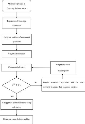
We obtain the score vector $v=(v_1,v_2,\dots ,v_m)$ of the probability degree matrix $P$ from the above equation. Finally, we rank the alternative scheme scores according to $v_f(f=1,2,\dots ,m)$ and choose the best alternative $a_l.$ Figure 1 shows the above-described process of the FGDM framework, which is proposed in this study.

Figure 1. Multiple-attribute group decision-making process for project financing.

Source: drawn by authors themselves.

4. Case study

Here, a case is used to illustrate the interaction and judgment process in FGDM.

4.1. Background description

The Newly built Chengdu Tianfu International Airport will help Chengdu integrate into global resource networks. For Jianyang, where the airport is to be located, this is an important development opportunity. The Airport Avenue would connect Jianyang City and Tianfu Airport. This development has strategic significance for Jianyang’s regional economy. To construct the Airport Avenue, local government has proposed three alternative financing schemes $a_l\left(l=1,\mathrm{}2,\mathrm{}3\right).$ Before choosing the final financing scheme, discussion and evaluation are essential.

Scheme 1. Issuing bonds of 1.5 billion yuan and setting the bond maturity to five years. At the same time, no more than 30% of the funds raised from the project's proceeds bonds will be used for supplementary flows. The comprehensive financing rate will be 9.8%.

Scheme 2. Creating the Jianyang Investment and Construction Fund. The 5-year benchmark interest rate of comprehensive financing cost is within 45%, and the total investment will be 2 billion yuan. The subscription method for units in the fund would be that the fund manager initiates subscriptions to financial institutions and other investors.

Scheme 3. Loaning a total amount of 1.6-billion-yuan from commercial banks. The comprehensive financing cost is 6.0% per year and the financing period is 6 years. After the loan is issued, the principal is returned once every 6 months after the grace period and the service fee is 3.0% per year.

To further analyze and evaluate each scheme, the evaluation index system for the financing scheme has been established according to Alonso (2013), Chang (2014) and Sahi et al. (2013). This is shown in Table 1.

Table 1. Evaluation index system of the financing scheme.

Comprehensive Index	Basic Index
Financing economy (${\mathit{y}}_1$)	Financing cost ($e_1$)
	Financing return ($e_2$)
	Financing scale ($e_3$)
Financing risk (${\mathit{y}}_2$)	Funding risk$(e_4$)
	Interest rate risk$(e_5$)
	Inflation risk $(e_6$)
Financing feasibility (${\mathit{y}}_3$)	Financing appeal$(e_7$)
	Financing procedure$(e_8$)
	Financing policy$(e_9$)
Financing reliability (${\mathit{y}}_4$)	Financing model$(e_{10}$)
	Funding plan$(e_{11}$)
	Financing speed$(e_{12}$)

Source: calculated by authors themselves.

Let four evaluation experts $V_q\left(q=1,\mathrm{}2,\mathrm{}3,\mathrm{}4\right)$ evaluate schemes $a_l\left(l=1,\mathrm{}2,\mathrm{}3\right)$ according to the evaluation index system. At the same time, the experts hope that their consensus coefficient is above 0.95 (${\xi }^{\mathrm{*}}\ge 0.95$). We first consider $\lambda =0.8.$ To avoid the subjectivity of the value of $\lambda ,$ the robustness test is further conducted by changing the value of $\lambda .$

The evaluation expert $V_1$’s preliminary judgment information of each scheme is shown in Table 2. The preliminary evaluation information of the remaining evaluation experts is shown in Appendix A.

Table 2. Expert $V_1$’s evaluation of each scheme.

（1）Comprehensive Index $y_1$

Basic Index	${\mathit{e}}_1$	${\mathit{e}}_2$	${\mathit{e}}_3$
${\mathit{a}}_1$	($H_2,0.6$)($H_3,0.2$)($H_4,0.2$)	($H_2,0.7$)($H_3,0.2$)($\mathrm{}H,$0.1)	($H_3,0.6$)$(H_4,0.2$)($H,$0.2)
${\mathit{a}}_2$	($H_3,0.9$)($H_4,0.1$)	($H_3,0.5$)$(H_4,0.4$)($\mathrm{}H,$0.1)	($H_4,0.2$)$(H_5,0.8$)
${\mathit{a}}_3$	$(H_2,0.1$)($H_3,0.3$) ($H_4,0.4)$	($H_3,0.3$)$(H_4,0.2$)($\mathrm{}H,$0.5)	($H_2,0.5$)$(H_3,0.5$)

（2）Comprehensive Index $y_2$

Basic Index	${\mathit{e}}_4$	${\mathit{e}}_5$	${\mathit{e}}_6$
${\mathit{a}}_1$	($H_1,0.6$)$(H_3,0.3$)($H,0.1$)	($H_3,0.6$)$(H_4,0.3$)($H,0.1$)	($H_3,0.5$)$(H_5,0.4$)($H,0.1$)
${\mathit{a}}_2$	($H_4,0.6$)$(H_5,0.3$)($H,0.1$)	($H_2,0.6$)$(H_3,0.2$)($H_4,0.2$)	($H_3,0.6$)$(H_4,0.2$)($H,0.2$)
${\mathit{a}}_3$	($H_2,0.3$)$(H_3,0.7$)	($H_2,0.3$)$(H_3,0.4$) ($H_4,0.2$)	($H_4,0.6$)$(H_5,0.4$)

（3）Comprehensive Index $y_3$

Basic Index	${\mathit{e}}_7$	${\mathit{e}}_8$	${\mathit{e}}_9$
${\mathit{a}}_1$	($H_2,0.5$)$(H_3,0.5$)	($H_3,0.4$)$(H_4,0.6$)	($H_2,0.3$)$(H_3,0.4$)($H_4,0.3$)
${\mathit{a}}_2$	($H_2,0.2$)$(H_3,0.6$)($H,0.2$)	($H_3,0.3$)$(H_4,0.7$)	($H_4,0.6$)$(H_5,03$)($H,0.1$)
${\mathit{a}}_3$	($H_1,0.5$)$(H_2,0.3$)($H,0.2$)	($H_3,0.4$)$(H_4,0.6$) ($H,0.2$)	($H_1,0.5$)$(H_2,0.4$)($H,0.1$)

（4）Comprehensive Index $y_4$

Basic Index	${\mathit{e}}_{10}$	${\mathit{e}}_{11}$	${\mathit{e}}_{12}$
${\mathit{a}}_1$	($H_4,0.7$)$(H_5,0.3$)	($H_3,0.3$)$(H_4,0.6$)($H,0.1$)	($H_3,0.5$)$(H_4,0.3$)$\mathrm{}(H_5,0.2$)
${\mathit{a}}_2$	($H_2,0.6$)$(H_3,0.4$)	($H_2,0.5$)$(H_3,0.4$)($H,0.1$)	($H_3,0.4$)$(H_4,0.3$)($H,0.3$)
${\mathit{a}}_3$	($H_3,0.8$)$(H_4,0.2$)	($H_4,0.4$)$(H_5,0.5$)($H,0.1$)	($H_2,0.5$)$(H_5,0.1$)($H,0.4$)

Source: calculated by authors themselves.

4.2. Aggregating assessments via evidence reasoning

Evaluating the alternative schemes can be computed according to the FGDM process proposed in this study and depicted in Figure 1. This process includes the following steps.

Step 1. Obtain judgment matrix for the evaluation experts

$p_i^{\left(q\right)\left(1\right)}$ is used as the linguistic decision matrix of the expert $V_q$($q=1,\mathrm{}2,\mathrm{}3,\mathrm{}4$) for the $i$ th $(i=1,\mathrm{}2,\mathrm{}3,\mathrm{}4)$ comprehensive attribute in the first round of evaluation. We can obtain the linguistic decision of evaluation experts in the first round using equation $S^{\left(k_i\right)}{p}^{(k_i)}*S^{\left(k_i\right)}{p}^{\left(k_j\right)}=H_{p^{(k_i)}*i+p^{(k_j)}*j}.$ The linguistic decision matrix of the evaluation expert $V_1$ is shown below. The linguistic decision matrix of the other evaluation experts is shown in Appendix B. $$p_1^{\left(1\right)\left(1\right)}=\left(\begin{array}{ccc}{H}_{2.6}& H_{2.3}& H_{3.2}\\ H_{3.1}& H_{3.4}& H_{4.8}\\ H_{3.3}& H_{3.2}& H_{2.5}\end{array}\right)\mathrm{}{p}_2^{\left(1\right)\left(1\right)}=\left(\begin{array}{ccc}{H}_{1.8}& H_{3.3}& H_{3.8}\\ H_{4.2}& H_{2.6}& H_{3.2}\\ H_{2.7}& H_{2.9}& H_{4.4}\end{array}\right)$$ $$p_3^{\left(1\right)\left(1\right)}=\left(\begin{array}{ccc}{H}_{2.5}& H_{3.6}& H_{3.0}\\ H_{2.8}& H_{3.7}& H_{4.2}\\ H_{1.7}& H_{3.2}& H_{1.6}\end{array}\right)\mathrm{}{p}_4^{\left(1\right)\left(1\right)}=\left(\begin{array}{ccc}{H}_{4.3}& H_{3.6}& H_{3.7}\\ H_{2.4}& H_{2.5}& H_{3.3}\\ H_{3.2}& H_{4.4}& H_{2.7}\end{array}\right)$$

Step 2. Determinate the experts’ weights

According to the evaluation expert’s linguistic decision matrix, the evaluation experts’ subjective weights and the similarities between experts can be calculated according to the equations (18)(18) $${\theta }_q^1=\frac{{\mathit{CHWI}}_q\mathrm{*}(n-Q_q)}{{\sum }_{q=1}^N{\mathit{CHWI}}_q\mathrm{*}(n-Q_q)}$$(18) and (19)(19) $$v_{qk}=\frac{\mathrm{vec}\left(p^{\left(q\right)\left(\delta \right)}\right)·\mathrm{vec}\left(p^{\left(k\right)\left(\delta \right)}\right)}{\Vert \mathrm{vec}\left(p^{\left(q\right)\left(\delta \right)}\right)\Vert ·\Vert \mathrm{vec}\left(p^{\left(k\right)\left(\delta \right)}\right)\Vert }\left(q,k=1,\mathrm{}2,\dots ,N\right).$$(19) . The results are shown in Table 3.

Table 3. Evaluation experts’ subjective weights for the evaluation indexes.

	${\mathit{y}}_1$	${\mathit{y}}_2$	${\mathit{y}}_3$	${\mathit{y}}_4$
${\mathit{V}}_1$	0.1759	0.2224	0.2632	0.2418
${\mathit{V}}_2$	0.1696	0.2487	0.2673	0.2653
${\mathit{V}}_3$	0.2073	0.1959	0.1794	0.2256
${\mathit{V}}_4$	0.4471	0.3329	0.2438	0.2668

Source: calculated by authors themselves.

At the same time, the similarities between the evaluation experts’ judgments are obtained using the equation (20)(20) $$v_q=\sum _{k=1,k\ne q}^N{v}_{qk}\left(k=1,\mathrm{}2,\dots ,N\right).$$(20) and are shown in Table 4.

Table 4. Similarities between experts’ judgments.

	${\mathit{V}}_1$	${\mathit{V}}_2$	${\mathit{V}}_3$	${\mathit{V}}_4$
${\mathit{V}}_1$	1	0.9886	0.9806	0.8974
${\mathit{V}}_2$	0.9886	1	0.9807	0.8932
${\mathit{V}}_3$	0.9806	0.9807	1	0.9223
${\mathit{V}}_4$	0.8974	0.8932	0.9223	1

Source: calculated by authors themselves.

The total weight of the evaluation experts is calculated by the equation (22)(22) $${\theta }_q=\lambda {\theta }_q^1+\left(1-\lambda \right){\theta }_q^2\left(q=1,\mathrm{}2,\dots ,N\right).$$(22) . The consensus judgment is obtained using the equation (23)(23) $${\xi }^{\delta }=\frac{{\sum }_{q=1}^N{\sum }_{k=1}^N{v}_{qk}}{N\left(N-1\right)}\left(q,k=1,\mathrm{}2,\dots ,N;q\ne k\right).$$(23) . The results are shown in Table 5.

Table 5. Evaluation expert weights and consensus coefficient.

	Subjective weigh	Objective weight	Total weight
${\mathit{V}}_1$	0.2259	0.2531	0.2340
${\mathit{V}}_2$	0.2377	0.2527	0.2422
${\mathit{V}}_3$	0.2275	0.2546	0.2356
${\mathit{V}}_4$	0.3227	0.2395	0.2977
Consensus coefficient	0.9438

Source: calculated by authors themselves.

Step 3. Consensus judgment

Calculating the consensus coefficient of the evaluation experts shows that the consensus level is not reached because ${\xi }^1<{\xi }^{\mathrm{*}}.$ Therefore, we continue with Step 4.

Step 4. Interaction process

The fourth evaluation expert has the minimum weight in Table 6. This indicates that his or her information may have consistency issues. The low similarities between the fourth expert and the other evaluation experts indicates that his or her information is extreme. Therefore, the expert$\mathrm{}{V}_4$ needs to modify his or her judgment information.

Table 6. Expert $V_4$’s evaluation of each scheme.

（1）Comprehensive Index $y_1$

Basic Index	${\mathit{e}}_1$	${\mathit{e}}_2$	${\mathit{e}}_3$
${\mathit{a}}_1$	($H_4,0.2$)$(H_5,0.8$)	($H_4,0.6$)$(H_5,0.3$)($H,0.1$)	($H_4,0.2$)$(H_5,0.8$)
${\mathit{a}}_2$	($H_4,0.3$)$(H_5,0.7$)	($H_3,0.4$)$(H_4,0.2$)$(H_5,0.4$)	($H_2,0.6$)$(H_3,0.4$)
${\mathit{a}}_3$	($H_4,0.3$)$(H_5,0.5$)($H,0.2$)	($H_2,0.1$)$(H_3,0.3$)$(H_4,0.6$)	($H_3,0.5$)$(H_4,0.5$)

（2）Comprehensive Index $y_2$

Basic Index	${\mathit{e}}_4$	${\mathit{e}}_5$	${\mathit{e}}_6$
${\mathit{a}}_1$	($H_2,0.2$)$(H_4,0.8$)	($H_3,0.8$)$(H_4,0.2$)	($H_2,0.6$)$(H_3,0.3$)($H,0.1$)
${\mathit{a}}_2$	($H_1,0.5$)$(H_2,0.3$)($H,0.2$)	($H_3,0.6$)$(H_4,0.3$)($H,0.1$)	($H_4,0.2$)$(H_5,0.7$)($H,0.1$)
${\mathit{a}}_3$	($H_3,0.2$)$(H_4,0.4$)$(H_5,0.4$)	($H_3,0.2$)$(H_5,0.8$)	($H_2,0.7$)$(H_3,0.3$)

（3）Comprehensive Index ${\mathit{y}}_3$

Basic Index	${\mathit{e}}_7$	${\mathit{e}}_8$	${\mathit{e}}_9$
${\mathit{a}}_1$	($H_2,0.5$)$(H_3,0.5$)	($H_3,0.4$)$(H_4,0.5$)($H,0.1$)	($H_2,0.2$)$(H_3,0.6$)($H_4,0.2$)
${\mathit{a}}_2$	($H_2,0.3$)$(H_3,0.6$)($H,0.1$)	($H_2,0.2$)$(H_3,0.6$)($H,0.2$)	($H_2,0.8$)$(H_3,0.1$)($H,0.1$)
${\mathit{a}}_3$	($H_4,0.2$)$(H_5,0.7$)($H,0.1$)	($H_2,0.4$)$(H_3,0.6$)	($H_3,0.3$)$(H_4,0.2$)$\mathrm{}(H_4,0.5$)

（4）Comprehensive Index $y_4$

Basic Index	${\mathit{e}}_{10}$	${\mathit{e}}_{11}$	${\mathit{e}}_{12}$
${\mathit{a}}_1$	($H_2,0.5$)$(H_3,0.5$)	($H_3,0.3$)$(H_4,0.7$)	($H_3,0.5$)$(H_4,0.2$)($H,0.3$)
${\mathit{a}}_2$	($H_3,0.7$)$(H_4,0.3$)	($H_3,0.2$)$(H_4,0.6$)($H,0.2$)	($H_3,0.5$)$(H_4,0.3$)($H,0.2$)
${\mathit{a}}_3$	($H_4,0.3$)$(H_5,0.7)$	($H_3,0.4$)($H_4,0.3$)$(H_5,0.3$)	($H_4,0.3$)$(H_5,0.1$)($H,0.6$)

Source: calculated by authors themselves.

The corresponding attribute judgment information is updated as follows: $$p_1^{\left(4\right)\left(2\right)}=\left(\begin{array}{ccc}{H}_{4.8}& H_{4.2}& H_{4.8}\\ H_{4.7}& H_{4.0}& H_{2.4}\\ H_{4.3}& H_{3.5}& H_{3.5}\end{array}\right)\mathrm{}{p}_2^{\left(4\right)\left(2\right)}=\left(\begin{array}{ccc}{H}_{3.8}& H_{3.2}& H_{2.4}\\ H_{1.7}& H_{3.3}& H_{4.6}\\ H_{4.2}& H_{4.6}& H_{2.3}\end{array}\right)$$ $$p_3^{\left(4\right)\left(2\right)}=\left(\begin{array}{ccc}{H}_{2.5}& H_{3.5}& H_{3.0}\\ H_{2.7}& H_{2.8}& H_{2.2}\\ H_{4.6}& H_{2.6}& H_{4.2}\end{array}\right)\mathrm{}{p}_4^{\left(4\right)\left(2\right)}=\left(\begin{array}{ccc}{H}_{2.5}& H_{3.7}& H_{3.2}\\ H_{3.3}& H_{3.6}& H_{3.3}\\ H_{4.7}& H_{3.9}& H_{3.5}\end{array}\right)$$

The adjusted similarities between experts, expert weights, and agreement coefficients are re-calculated. The updated similarities between experts are shown in Table 7.

Table 7. Revised similarities between experts.

	${\mathit{V}}_1$	${\mathit{V}}_2$	${\mathit{V}}_3$	${\mathit{V}}_4$
${\mathit{V}}_1$	1	0.9886	0.9806	0.9164
${\mathit{V}}_2$	0.9886	1	0.9807	0.9227
${\mathit{V}}_3$	0.9806	0.9807	1	0.9351
${\mathit{V}}_4$	0.9164	0.9227	0.9351	1

Source: calculated by authors themselves.

We calculate the objective weights of the evaluation experts according to the equations (22)(22) $${\theta }_q=\lambda {\theta }_q^1+\left(1-\lambda \right){\theta }_q^2\left(q=1,\mathrm{}2,\dots ,N\right).$$(22) and (23)(23) $${\xi }^{\delta }=\frac{{\sum }_{q=1}^N{\sum }_{k=1}^N{v}_{qk}}{N\left(N-1\right)}\left(q,k=1,\mathrm{}2,\dots ,N;q\ne k\right).$$(23) . The results are shown in Table 8.

Table 8. Revised evaluation expert weights and consensus coefficient.

	Subjective weigh	Objective weight	Total weight
${\mathit{V}}_1$	0.2597	0.2521	0.2574
${\mathit{V}}_2$	0.2721	0.2526	0.2662
${\mathit{V}}_3$	0.2647	0.2530	0.2612
${\mathit{V}}_4$	0.2181	0.2423	0.2254
Consensus coefficient	0.9540

Source: calculated by authors themselves.

Calculating the consensus coefficient of the evaluation experts shows that ${\xi }^2>{\xi }^{\mathrm{*}},$ which means the required consensus level has been achieved.

Step 5. Obtain attributes weights

Next, we calculate the gray correlation of the attribute and the attribute importance according to the equations (25)–(29). The relative results are shown in Table 9.

Table 9. Attributes’ relative weights.

Comprehensive attributes	Basic attributes	Gray correlation	Attributes’ relative weights
${\mathit{y}}_1$	$e_1$	0.8925	0.3542
	$e_2$	0.8091	0.3211
	$e_3$	0.8178	0.3246
${\mathit{y}}_2$	$e_4$	0.9182	0.3545
	$e_5$	0.8059	0.3112
	$e_6$	0.8658	0.3343
${\mathit{y}}_3$	$e_7$	0.7760	0.3141
	$e_8$	0.8129	0.3291
	$e_9$	0.8817	0.3569
${\mathit{y}}_4$	$e_{10}$	0.8636	0.3694
	$e_{11}$	0.7294	0.3120
	$e_{12}$	0.7447	0.3186

Source: calculated by authors themselves.

Step 6. Aggregating assessments

We can obtain the result on the multiple attributes according to the equations (30)–(41). Table 10 shows the result after information is aggregated. These are the evaluation experts’ comprehensive evaluation results of the alternative schemes.

Table 10. Comprehensive evaluation results provided by evaluation experts.

	${\mathit{H}}_1$	${\mathit{H}}_2$	${\mathit{H}}_3$	${\mathit{H}}_4$	${\mathit{H}}_5$	$\mathit{H}$
${\mathit{a}}_1$	0.0201	0.0808	0.4232	0.3155	0.0664	0.0936
${\mathit{a}}_2$	0.0269	0.0915	0.4171	0.2953	0.0740	0.0952
${\mathit{a}}_3$	0.0087	0.1462	0.3719	0.2413	0.1184	0.1135

Source: calculated by authors themselves.

Step 7. Compare alternative schemes

The comprehensive score of the experts is determined using equations (43)–(44), then this result is summed. Finally, the weights of the experts are integrated to obtain the final score of each financing scheme, as shown in Table 11.

Table 11. Final utility value of each scheme.

	Minimum utility value	Maximum utility value
${\mathit{a}}_1$	0.5349	0.6285
${\mathit{a}}_2$	0.5269	0.6221
${\mathit{a}}_3$	0.5218	0.6354

Source: calculated by authors themselves.

The comprehensive scores of each scheme are obtained according to equations (43)–(44). The final scores are as follows:

The alternative financing schemes are ranked as $a_2\succ a_1\succ a_3$ according to the final score. Therefore, the best financing scheme is the second alternative.

4.3. Further analysis

In this subsection, three different approaches are used to verify the validity of our framework. One is to test the validity of the double interaction, the second is to show the effectiveness of the weight setting process, and the last one is the comparative analyses between the proposed approach in this study and the existing approaches of PLTS and ER. Through the robustness tests given below, it is proven that the method proposed in our study is not only effective, but also stable.

4.3.1. Validity of interaction between experts

In the decision-making process, significant differences in judgment information between experts can be avoided by the interaction between experts. However, if the interaction is not considered, the relative consistency between subjective weights and objective weights cannot be ensured, the total weights in Table 5 will be the final weights, and the result is listed in Table 12 accordingly. Here, the ranking is $a_2\succ a_3\succ a_1,$ which is different from the one we obtained in Table 13.

Table 12. Final score of each scheme without interaction.

	${\mathit{a}}_1$	${\mathit{a}}_2$	${\mathit{a}}_3$
Score	0.2542	0.3273	0.2573

Source: calculated by authors themselves.

Table 13. Final score of each financing scheme.

	${\mathit{a}}_1$	${\mathit{a}}_2$	${\mathit{a}}_3$
Score	0.2589	0.3301	0.2508

Source: calculated by authors themselves.

To verify the validity of the interaction between experts, we change the value of $\lambda ,$ which is treated as a subjective variable in the parameter setting. The results of the comparison are shown in Table 14.

Table 14. Ordering between schemes with different $\lambda .$

Value of $\mathbf{\lambda }$	Ranking of alternative schemes
	Without interaction	With interaction
$\mathbf{\lambda }=0$	$a_2\succ a_1\succ a_3$	$a_2\succ a_1\succ a_3$
$\mathbf{\lambda }=0.1$	$a_2\succ a_1\succ a_3$	$a_2\succ a_1\succ a_3$
$\mathbf{\lambda }=0.2$	$a_2\succ a_1\succ a_3$	$a_2\succ a_1\succ a_3$
$\mathbf{\lambda }=0.3$	$a_2\succ a_1\succ a_3$	$a_2\succ a_1\succ a_3$
$\mathbf{\lambda }=0.4$	$a_2\succ a_1\succ a_3$	$a_2\succ a_1\succ a_3$
$\mathbf{\lambda }=0.5$	$a_2\succ a_1\succ a_3$	$a_2\succ a_1\succ a_3$
$\mathbf{\lambda }=0.6$	$a_2\succ a_3\succ a_1$	$a_2\succ a_1\succ a_3$
$\mathbf{\lambda }=0.7$	$a_2\succ a_3\succ a_1$	$a_2\succ a_1\succ a_3$
$\mathbf{\lambda }=0.8$	$a_2\succ a_3\succ a_1$	$a_2\succ a_1\succ a_3$
$\mathbf{\lambda }=0.9$	$a_2\succ a_3\succ a_1$	$a_2\succ a_1\succ a_3$
$\mathbf{\lambda }=1$	$a_2\succ a_3\succ a_1$	$a_2\succ a_1\succ a_3$

Source: calculated by authors themselves.

In the absence of interaction between experts, the ranking of alternative schemes is unstable. When $\lambda \le 0.5,$ the ranking of the alternatives is $a_2\succ a_1\succ a_3.$ However, the situation differs once $\lambda \ge 0.6,$ that is $a_2\succ a_3\succ a_1.$ One possible explanation for this is that non-interaction is more likely to lead to a large difference between subjective weights and objective weights. With the increase of the subjective weights ($\lambda$) ratio, the ranking of alternative schemes may change. It is difficult for decision makers to make optimal decisions under such unreliable results. As a result, they could miss out on the best financing scheme and may opt for a sub-optimal choice. However, once we allow for an interaction between experts, the ranking of schemes remains stable, regardless of the changes in$\lambda .$ Therefore, we think that experts’ judgments are more stably through experts’ interaction, and the ranking results are more reliable, and the stability of the results is stronger.

4.3.2. Effectiveness of weight setting

Subsection 3.3 shows that the probability of uncertain information can be assigned to any level. Accordingly, the uncertain information also has a corresponding score in the probability term score setting process. Considering the experts’ uncertainty degree $Q_q$ based on uncertain information could avoid the situation in which experts are not clear about the attribute information, but the subjective weight applied to the attribute is high through uncertain information. To verify the superiority of weight setting in this paper, we compare the results of the two processes by considering the $Q_q$ and not considering in Table 15.

Table 15. Ordering between schemes with different $\lambda .$

Value of $\mathbf{\lambda }$	Ranking of alternative schemes
	With uncertainty degree	Without uncertainty degree
$\mathbf{\lambda }=0$	$a_2\succ a_1\succ a_3$	$a_2\succ a_1\succ a_3$
$\mathbf{\lambda }=0.1$	$a_2\succ a_1\succ a_3$	$a_2\succ a_1\succ a_3$
$\mathbf{\lambda }=0.2$	$a_2\succ a_1\succ a_3$	$a_2\succ a_1\succ a_3$
$\mathbf{\lambda }=0.3$	$a_2\succ a_1\succ a_3$	$a_2\succ a_1\succ a_3$
$\mathbf{\lambda }=0.4$	$a_2\succ a_1\succ a_3$	$a_2\succ a_1\succ a_3$
$\mathbf{\lambda }=0.5$	$a_2\succ a_1\succ a_3$	$a_2\succ a_1\succ a_3$
$\mathbf{\lambda }=0.6$	$a_2\succ a_1\succ a_3$	$a_2\succ a_1\succ a_3$
$\mathbf{\lambda }=0.7$	$a_2\succ a_3\succ a_1$	$a_2\succ a_1\succ a_3$
$\mathbf{\lambda }=0.8$	$a_2\succ a_3\succ a_1$	$a_2\succ a_1\succ a_3$
$\mathbf{\lambda }=0.9$	$a_2\succ a_3\succ a_1$	$a_2\succ a_1\succ a_3$
$\mathbf{\lambda }=1$	$a_2\succ a_3\succ a_1$	$a_2\succ a_1\succ a_3$

Source: calculated by authors themselves.

The ranking of alternative schemes is also unstable under interaction without uncertainty degrees. This lack of stability may cause confusion for the decision maker trying to make a final decision. However, the above situation will be improved once we consider the uncertainty degree in the weight setting process. No matter how $\lambda$ changes, the ranking of schemes is always $a_2\succ a_1\succ a_3.$ This is because we consider the uncertainty degree and reduce the impact this has on the weight setting process, thus the stability of the scheme ranking results improves. Based on the comparison in Table 15, one fact can be seen: considering the uncertainty degree, no matter how the value of $\lambda$ changes, the final sorting results will be consistent.

4.3.3. Comparative analysis

For the FGDM, we make some comparative analyses between the proposed approach in this study and the existing approaches of PLTS and ER with interaction between experts. The results of the comparison are shown in Table 16 below.

Table 16. Ordering between schemes with different approaches.

Value of $\mathit{\rho }$	Ranking of alternative schemes under different approaches
	PLTS approach	ER with interaction	The proposed approach
$\mathit{\rho }=0$	$a_1\succ a_2\succ a_3$	$a_2\succ a_1\succ a_3$	$a_2\succ a_1\succ a_3$
$\mathit{\rho }=0.1$	$a_1\succ a_2\succ a_3$	$a_2\succ a_1\succ a_3$	$a_2\succ a_1\succ a_3$
$\mathit{\rho }=0.2$	$a_1\succ a_2\succ a_3$	$a_2\succ a_1\succ a_3$	$a_2\succ a_1\succ a_3$
$\mathit{\rho }=0.3$	$a_1\succ a_2\succ a_3$	$a_2\succ a_3\succ a_1$	$a_2\succ a_1\succ a_3$
$\mathit{\rho }=0.4$	$a_1\succ a_2\succ a_3$	$a_2\succ a_3\succ a_1$	$a_2\succ a_1\succ a_3$
$\mathit{\rho }=0.5$	$a_1\succ a_3\succ a_2$	$a_2\succ a_3\succ a_1$	$a_2\succ a_1\succ a_3$
$\mathit{\rho }=0.6$	$a_1\succ a_3\succ a_2$	$a_2\succ a_3\succ a_1$	$a_2\succ a_1\succ a_3$
$\mathit{\rho }=0.7$	$a_1\succ a_3\succ a_2$	$a_2\succ a_3\succ a_1$	$a_2\succ a_1\succ a_3$
$\mathit{\rho }=0.8$	$a_1\succ a_3\succ a_2$	$a_2\succ a_3\succ a_1$	$a_2\succ a_1\succ a_3$
$\mathit{\rho }=0.9$	$a_1\succ a_3\succ a_2$	$a_2\succ a_3\succ a_1$	$a_2\succ a_1\succ a_3$
$\mathit{\rho }=1$	$a_1\succ a_3\succ a_2$	$a_2\succ a_3\succ a_1$	$a_2\succ a_1\succ a_3$

Source: calculated by authors themselves.

It can be seen from Table 16 that the PLTS is applied, the ranking of alternative schemes will change for different values of $\rho .$ It is confusing for decision makers to make a scheme selection in facing ranking changes of alternative schemes. At the same time, we can still see that considering only the first interaction is insufficient, this ranking result will also change with the change of $\rho .$ By contrast, the double interaction proposed in this paper will keep the ranking schemes unchanged under different values of $\rho .$ Thus, the double interaction framework is validated, and the proposed approach is effective.

5. Conclusions

FGDM is crucial to the deployment and construction of major national engineering projects. The main participants in the FGDM process are evaluation experts. The decision analysis process must thus pay special attention to balancing the weights among experts. At the same time, when evaluation experts are asked for evaluations, they may be hesitant to choose between several linguistic terms. Therefore, how to effectively solve the above problems is very important in the FGDM process. However, most of the existing research on project financing focuses on the set of weights for decision alternatives but understanding how to adjust them to reflect an uncertain environment is not well studied. In addition, past research rarely considers the interactions between experts and between parameters under uncertain evaluation information.

To solve these problems, we combine ER and PLTS to process uncertain information, and further propose a double interaction-based multiple aggregation method to deal with inconsistent assessments. The case study shows the effectiveness and stability of the methodology under a double interaction-based decision-making scenario with uncertain information. It is expected that this framework will become a useful tool for FGDM.

Our research suggests that evaluation experts should provide specific probability values for an evaluation level. But we do not account for situations where it is difficult for experts to give an accurate probability value. Therefore, Further research can consider using intervals to represent incomplete information in the probability distribution.

Disclosure statement

No potential conflict of interest was reported by the authors.

Appendix A

Table A1. Expert $V_2$’s evaluation of each scheme.

（1）Comprehensive Index $y_1$

Basic Index	${\mathit{e}}_1$	${\mathit{e}}_2$	${\mathit{e}}_3$
${\mathit{a}}_1$	($H_3,0.6$)($\mathrm{}{H}_4,0.4$)	($H_2,0.3$)($\mathrm{}{H}_4,0.6$)($H,0.1$)	($H_3,0.4$)($\mathrm{}{H}_4,0.5$)($H,0.1$)
${\mathit{a}}_2$	($H_2,0.3$)($\mathrm{}{H}_3,0.7$)	($H_4,0.8$)($\mathrm{}{H}_5,0.2$)	($H_4,0.5$)($\mathrm{}{H}_5,0.3$)($H,0.2$)
${\mathit{a}}_3$	($\mathrm{}{H}_2,0.5$)($H_3,0.4$)($H,0.1$)	($H_3,0.3$)($\mathrm{}{H}_4,0.4$) ($H,0.3$)	($H_2,0.6$)($\mathrm{}{H}_3,0.4$)

（2）Comprehensive Index $y_2$

Basic Index	${\mathit{e}}_4$	${\mathit{e}}_5$	${\mathit{e}}_6$
${\mathit{a}}_1$	($H_1,0.5$)($\mathrm{}{H}_2,0.3$)($H_3,0.2$)	($H_3,0.5$)($\mathrm{}{H}_4,0.4$)($H,0.1$)	($H_3,0.4$)($\mathrm{}{H}_4,0.5$)($H_5,0.1$)
${\mathit{a}}_2$	($H_3,0.4$)($\mathrm{}{H}_4,0.6$)	($H_2,0.7$)($\mathrm{}{H}_3,0.3$)	($H_3,0.5$)($\mathrm{}{H}_4,0.4$)($H,0.1$)
${\mathit{a}}_3$	($H_3,0.8$)($H,0.2$)	($H_2,0.4$)($\mathrm{}{H}_3,0.4$)($H,0.2$)	($H_3,0.1$)($\mathrm{}{H}_4,0.9$)

（3）Comprehensive Index ${\mathit{y}}_3$

Basic Index	${\mathit{e}}_7$	${\mathit{e}}_8$	${\mathit{e}}_9$
${\mathit{a}}_1$	($H_2,0.3$)($\mathrm{}{H}_3,0.7$)	($H_3,0.6$)($\mathrm{}{H}_4,0.3$)($\mathrm{}H,0.1$)	($H_2,0.1$)($\mathrm{}{H}_3,0.6$)($H_4,0.3$)
${\mathit{a}}_2$	($H_2,0.5$)($\mathrm{}{H}_3,0.4$)($H,0.1$)	($H_4,0.8$)($\mathrm{}{H}_5,0.2$)	($H_4,0.5$)($\mathrm{}{H}_5,04$)($H,0.1$)
${\mathit{a}}_3$	($H_1,0.3$)($\mathrm{}{H}_2,0.6$)($H,0.1$)	($H_3,0.5$)($\mathrm{}{H}_4,0.5$)	($H_1,0.7$)($\mathrm{}{H}_2,0.3$)

（4）Comprehensive Index $y_4$

Basic Index	${\mathit{e}}_{10}$	${\mathit{e}}_{11}$	${\mathit{e}}_{12}$
${\mathit{a}}_1$	($H_4,0.8$)($\mathrm{}{H}_5,0.2$)	($H_3,0.4$)($\mathrm{}{H}_4,0.5$)($H,0.1$)	($H_4,0.4$)($\mathrm{}{H}_5,0.3$)($H,0.3$)
${\mathit{a}}_2$	($H_2,0.5$)($\mathrm{}{H}_3,0.5$)	($H_2,0.4$)($\mathrm{}{H}_3,0.6$)	($H_1,0.7$)($\mathrm{}{H}_3,0.3$)
${\mathit{a}}_3$	($H_2,0.2$)($\mathrm{}{H}_3,0.3)$($\mathrm{}{H}_4,0.5$)	($H_3,0.2$)($\mathrm{}{H}_5,0.7$)($H,0.1$)	($H_2,0.4$)($\mathrm{}{H}_5,0.2$)($H,0.4$)

Table A2. Expert $V_3$’s evaluation of each scheme.

（1）Comprehensive Index $y_1$

Basic Index	${\mathit{e}}_1$	${\mathit{e}}_2$	${\mathit{e}}_3$
${\mathit{a}}_1$	($H_2,0.5$)($\mathrm{}{H}_3,0.4$)($H,0.1$)	($H_2,0.4$)($\mathrm{}{H}_3,0.6$)	($H_3,0.6$)($\mathrm{}{H}_4,0.4$)
${\mathit{a}}_2$	($H_3,0.7$)($\mathrm{}{H}_4,0.3$)	($H_3,0.5$)($\mathrm{}{H}_4,0.5$)	($H_3,0.4$)($\mathrm{}{H}_4,0.5$)($H,0.1$)
${\mathit{a}}_3$	($\mathrm{}{H}_2,0.2$)($H_3,0.5$) ($H,0.3$)	($H_2,0.3$)($\mathrm{}{H}_3,0.7$)	($H_2,0.3$)($\mathrm{}{H}_3,0.6$)($H_4,0.1$)

（2）Comprehensive Index $y_2$

Basic Index	${\mathit{e}}_4$	${\mathit{e}}_5$	${\mathit{e}}_6$
${\mathit{a}}_1$	($H_1,0.2$)($\mathrm{}{H}_3,0.8$)	($H_2,0.2$)($\mathrm{}{H}_3,0.7$)($H,0.1$)	($H_3,0.2$)($\mathrm{}{H}_4,0.6$)($H,0.2$)
${\mathit{a}}_2$	($H_4,0.5$)($\mathrm{}{H}_5,0.4$)($H,0.1$)	($H_3,0.4$)($\mathrm{}{H}_4,0.6$)	($H_3,0.4$)($\mathrm{}{H}_4,0.4$)($H_5,0.2$)
${\mathit{a}}_3$	($H_2,0.3$)($\mathrm{}{H}_3,0.6$)($H,0.1$)	($H_2,0.3$)($\mathrm{}{H}_3,0.4$)($H_4,0.3$)	($H_4,0.2$)($\mathrm{}{H}_5,0.8$)

（3）Comprehensive Index ${\mathit{y}}_3$

Basic Index	${\mathit{e}}_7$	${\mathit{e}}_8$	${\mathit{e}}_9$
${\mathit{a}}_1$	($H_2,0.5$)($\mathrm{}{H}_3,0.5$)	($H_2,0.1$)($H_3,0.4$)($\mathrm{}{H}_4,0.5$)	($\mathrm{}{H}_3,0.7$)($H_4,0.3$)
${\mathit{a}}_2$	($\mathrm{}{H}_3,0.6$)($H_4,0.4$)	($H_3,0.1$)($\mathrm{}{H}_4,0.6$)($\mathrm{}{H}_5,0.3$)	($H_4,0.4$)($\mathrm{}{H}_5,0.4$)($H,0.2$)
${\mathit{a}}_3$	($H_1,0.3$)($\mathrm{}{H}_3,0.6$)($H,0.1$)	($H_2,0.4$)($\mathrm{}{H}_3,0.6$)	($H_2,0.2$)($\mathrm{}{H}_3,0.4$)($\mathrm{}{H}_4,0.4$)

（4）Comprehensive Index $y_4$

Basic Index	${\mathit{e}}_{10}$	${\mathit{e}}_{11}$	${\mathit{e}}_{12}$
${\mathit{a}}_1$	($\mathrm{}{H}_3,0.4$)($H_4,0.3$)($\mathrm{}{H}_5,0.3$)	($H_3,0.5$)($\mathrm{}{H}_4,0.4$)($H,0.1$)	($H_4,0.3$)($\mathrm{}{H}_5,0.4$) ($H,0.3$)
${\mathit{a}}_2$	($H_3,0.5$)($\mathrm{}{H}_4,0.5$)	($H_2,0.1$)($\mathrm{}{H}_3,0.5$)($H_4,0.4$)	($H_1,0.8$) ($H,0.2$)
${\mathit{a}}_3$	($H_3,0.4$)($\mathrm{}{H}_4,0.5)$($\mathrm{}H,0.1$)	($H_4,0.8$)($\mathrm{}{H}_5,0.2$)	($\mathrm{}{H}_4,0.4$)($H,0.6$)

Table A3. Expert $V_4$’s evaluation of each scheme.

（1）Comprehensive Index $y_1$

Basic Index	${\mathit{e}}_1$	${\mathit{e}}_2$	${\mathit{e}}_3$
${\mathit{a}}_1$	($H_1,0.6$)($\mathrm{}{H}_2,0.1$) ($H_3,0.2$)	($\mathrm{}{H}_1,0.6$)($\mathrm{}{H}_2,0.4$)	($H_2,0.8$)($\mathrm{}{H}_3,0.2$)
${\mathit{a}}_2$	($H_1,0.5$)($\mathrm{}{H}_2,0.2$) ($H_4,0.3$)	($H_1,0.4$)($H_3,0.4$)($H_4,0.2$)	($H_1,0.4$)($\mathrm{}{H}_2,0.6$)
${\mathit{a}}_3$	($H_1,0.5$)($\mathrm{}{H}_3,0.3$)($H,0.2$)	($H_2,0.1$)($\mathrm{}{H}_3,0.3$)($H_4,0.6$)	($H_1,0.4$)($\mathrm{}{H}_2,0.5$)($H_4,0.1$)

（2）Comprehensive Index $y_2$

Basic Index	${\mathit{e}}_4$	${\mathit{e}}_5$	${\mathit{e}}_6$
${\mathit{a}}_1$	($H_3,0.2$)($\mathrm{}{H}_4,0.8$)	($H_3,0.4$)($\mathrm{}{H}_4,0.2$) ($H_5,0.4$)	($H_2,0.6$)($\mathrm{}{H}_3,0.3$)($H,0.1$)
${\mathit{a}}_2$	($H_1,0.5$)($\mathrm{}{H}_2,0.3$)($H,0.2$)	($H_1,0.2$)($\mathrm{}{H}_3,0.5$)($H_4,0.3$)	($H_2,0.7$)($H_4,0.2$) ($H,0.1$)
${\mathit{a}}_3$	($H_1,0.6$)($H_2,0.2$)($\mathrm{}{H}_3,0.2$)	($H_3,0.2$)($\mathrm{}{H}_5,0.8$)	($H_1,0.7$)($\mathrm{}{H}_2,0.3$)

（3）Comprehensive Index ${\mathit{y}}_3$

Basic Index	${\mathit{e}}_7$	${\mathit{e}}_8$	${\mathit{e}}_9$
${\mathit{a}}_1$	($H_2,0.5$)($\mathrm{}{H}_3,0.5$)	($H_2,0.1$)($\mathrm{}{H}_3,0.4$)($\mathrm{}{H}_4,0.5$)	($H_2,0.2$)($H_3,0.6$)($H_4,0.2$)
${\mathit{a}}_2$	($H_2,0.3$)($\mathrm{}{H}_3,0.6$)($H,0.1$)	($H_2,0.2$)($\mathrm{}{H}_3,0.6$)($H,0.2$)	($H_2,0.8$)($H_3,0.1$)($H,0.1$)
${\mathit{a}}_3$	($H_4,0.2$)($\mathrm{}{H}_5,0.7$)($H,0.1$)	($H_1,0.2$)($\mathrm{}{H}_2,0.4$)($\mathrm{}{H}_3,0.4$)	($H_3,0.3$)($H_4,0.2$)($H_5,0.5$)

（4）Comprehensive Index $y_4$

Basic Index	${\mathit{e}}_{10}$	${\mathit{e}}_{11}$	${\mathit{e}}_{12}$
${\mathit{a}}_1$	($H_2,0.5$)($\mathrm{}{H}_3,0.5$)	($H_2,0.3$)($\mathrm{}{H}_3,0.3$)$(H_4,0.4$)	($H_2,0.4$)($\mathrm{}{H}_3,0.4$)($H_4,0.2$)
${\mathit{a}}_2$	($H_3,0.7$)($\mathrm{}{H}_4,0.3$)	($H_3,0.2$)($\mathrm{}{H}_4,0.6$)($H,0.2$)	($H_2,0.3$)($\mathrm{}{H}_3,0.5$)($H,0.2$)
${\mathit{a}}_3$	($H_4,0.3$)($\mathrm{}{H}_5,0.7)$	($H_3,0.4$)($H_4,0.3$)($\mathrm{}{H}_5,0.3$)	($H_1,0.3$)($\mathrm{}{H}_4,0.3$)($H,0.4$)

Appendix B

Evaluation expert $V_2$’s linguistic decision matrix: $$\begin{array}{cc}{p}_1^{\left(2\right)\left(1\right)}=\left(\begin{array}{ccc}{H}_{3.4}& H_{3.3}& H_{3.5}\\ H_{2.7}& H_{4.2}& H_{4.1}\\ H_{2.5}& H_{3.4}& H_{2.4}\end{array}\right)& p_2^{\left(2\right)\left(1\right)}=\left(\begin{array}{ccc}{H}_{1.7}& H_{3.4}& H_{3.7}\\ H_{3.6}& H_{2.3}& H_{3.4}\\ H_{3.2}& H_{2.6}& H_{3.9}\end{array}\right)\\ p_3^{\left(2\right)\left(1\right)}=\left(\begin{array}{ccc}{H}_{2.7}& H_{3.3}& H_{3.2}\\ H_{2.5}& H_{4.2}& H_{4.3}\\ H_{1.8}& H_{3.5}& H_{1.3}\end{array}\right)& p_4^{\left(2\right)\left(1\right)}=\left(\begin{array}{ccc}{H}_{4.2}& H_{3.5}& H_4\\ H_{2.5}& H_{2.6}& H_{1.6}\\ H_{3.3}& H_{4.4}& H_{3.0}\end{array}\right)\end{array}$$

Evaluation expert $V_3$’s linguistic decision matrix: $$\begin{array}{cc}{p}_1^{\left(3\right)\left(1\right)}=\left(\begin{array}{ccc}{H}_{2.5}& H_{2.6}& H_{3.4}\\ H_{3.3}& H_{3.5}& H_{3.5}\\ H_{2.8}& H_{2.7}& H_{2.8}\end{array}\right)& p_2^{\left(3\right)\left(1\right)}=\left(\begin{array}{ccc}{H}_{2.6}& H_{2.8}& H_{3.6}\\ H_{4.3}& H_{3.6}& H_{3.8}\\ H_{2.7}& H_{3.0}& H_{4.8}\end{array}\right)\\ p_3^{\left(3\right)\left(1\right)}=\left(\begin{array}{ccc}{H}_{2.5}& H_{3.4}& H_{3.3}\\ H_{3.4}& H_{4.2}& H_{4.2}\\ H_{2.4}& H_{2.6}& H_{3.2}\end{array}\right)& p_4^{\left(3\right)\left(1\right)}=\left(\begin{array}{ccc}{H}_{3.9}& H_{3.4}& H_{4.1}\\ H_{3.5}& H_{3.3}& H_{1.4}\\ H_{3.5}& H_{4.2}& H_{3.4}\end{array}\right)\end{array}$$

Evaluation expert $V_4$’s linguistic decision matrix: $$\begin{array}{cc}{p}_1^{\left(4\right)\left(1\right)}=\left(\begin{array}{ccc}{H}_{1.9}& H_{1.4}& H_{2.2}\\ H_{2.2}& H_{2.4}& H_{1.6}\\ H_{2.0}& H_{3.5}& H_{1.8}\end{array}\right)& p_2^{\left(4\right)\left(1\right)}=\left(\begin{array}{ccc}{H}_{3.8}& H_{4.0}& H_{2.4}\\ H_{1.7}& H_{2.9}& H_{2.5}\\ H_{1.6}& H_{4.6}& H_{1.3}\end{array}\right)\\ p_3^{\left(4\right)\left(1\right)}=\left(\begin{array}{ccc}{H}_{2.5}& H_{3.4}& H_{3.0}\\ H_{2.7}& H_{2.8}& H_{2.2}\\ H_{4.6}& H_{2.6}& H_{4.2}\end{array}\right)& p_4^{\left(4\right)\left(1\right)}=\left(\begin{array}{ccc}{H}_{2.5}& H_{3.1}& H_{2.8}\\ H_{3.3}& H_{3.6}& H_{2.7}\\ H_{4.7}& H_{3.9}& H_{2.7}\end{array}\right)\end{array}$$

References

- Alavipour, S. M. R., & Arditi, D. (2018). Impact of contractor’s optimized financing cost on project bid price. International Journal of Project Management, 36(5), 808–818. https://doi.org/10.1016/j.ijproman.2018.03.001
- Alonso, S. (2013). Temporal discounting and number representation. Journal of Behavioral Finance, 14(3), 240–251. https://doi.org/10.1080/15427560.2013.820188
- Bashiri, M., & Badri, H. (2011). A group decision making procedure for fuzzy interactive linear assignment programming. Expert Systems with Applications, 38(5), 5561–5568. https://doi.org/10.1016/j.eswa.2010.10.080
- Chang, Z. (2014). Financing new metros—The Beijing metro financing sustainability study. Transport Policy, 32, 148–155. https://doi.org/10.1016/j.tranpol.2014.01.009
- Chang, L. L., Li, M. J., & Jiang, J. (2013). A variable weight approach for evidential reasoning. Journal of Central South University, 20(8), 2202–2211. https://doi.org/10.1007/s11771-013-1725-2
- Chemmanur, T. J., & John, K. (1996). Optimal incorporation, structure of debt contracts, and limited-recourse project financing. Journal of Financial Intermediation, 5(4), 372–408. https://doi.org/10.1006/jfin.1996.0021
- Chen, Y., & Zhang, D. N. (2020). Evaluation of city sustainability using multi-criteria decision-making considering interaction among criteria in Liaoning province China. Sustainable Cities and Society, 59, 102211. https://doi.org/10.1016/j.scs.2020.102211
- Cheng, X., Gu, J., & Xu, Z. S. (2018). Venture capital group decision-making with interaction under probabilistic linguistic environment. Knowledge-Based Systems, 140, 82–91. https://doi.org/10.1016/j.knosys.2017.10.030
- Chin, K. S., Yang, J. B., Guo, M., & Lam, J. P. K. (2009). An evidential-reasoning-interval-based method for new product design assessment. IEEE Transactions on Engineering Management, 56(1), 142–156.
- Gou, X. J., Xu, Z. S., & Zhou, W. (2020). Interval consistency repairing method for double hierarchy hesitant fuzzy linguistic preference relation and application in the diagnosis of lung cancer. Economic Research-Ekonomska Istrazivanja, 34(1), 1–20.
- Grimsey, D., & Lewis, M. K. (2002). Evaluating the risks of public private partnerships for infrastructure projects. International Journal of Project Management, 20(2), 107–118. https://doi.org/10.1016/S0263-7863(00)00040-5
- Han, X. L., & Li, S. R. (1994). The priority method in view of consistency harmonious weight index. Systems Engineering-Theory Methodology Applications, 3(1), 41–45.
- Herrera, F., Herrera-Viedma, E., & Verdegay, J. L. (1997). A rational consensus model in group decision making using linguistic assessments. Fuzzy Sets and Systems, 88(1), 31–49. https://doi.org/10.1016/S0165-0114(96)00047-4
- Jiang, G., Lee, C. M., & Zhang, Y. (2005). Information uncertainty and expected returns. Review of Accounting Studies, 10(2-3), 185–221. https://doi.org/10.1007/s11142-005-1528-2
- Kissinger, G., Gupta, A., Mulder, I., & Unterstell, N. (2019). Climate financing needs in the land sector under the Paris Agreement: An assessment of developing country perspectives. Land Use Policy, 83, 256–269. https://doi.org/10.1016/j.landusepol.2019.02.007
- Kong, G., Xu, D. L., Yang, J. B., & Ma, X. (2015). Combined medical quality assessment using the evidential reasoning approach. Expert Systems with Applications, 42(13), 5522–5530. https://doi.org/10.1016/j.eswa.2015.03.009
- Lamont, O. (1997). Cash flow and investment: Evidence from internal capital markets. Journal of Financial Economics, 52(1), 83–109.
- Liu, Z. B., Gao, R., Zhou, C., & Ma, N. (2019). Two-period pricing and strategy choice for a supply chain with dual uncertain information under different profit risk levels. Computers & Industrial Engineering, 136, 173–186. https://doi.org/10.1016/j.cie.2019.07.029
- Lourenzutti, R., Krohling, R. A., & Reformat, M. Z. (2017). Choquet based TOPSIS and TODIM for dynamic and heterogeneous decision making with criteria interaction. Information Sciences, 408, 41–69. https://doi.org/10.1016/j.ins.2017.04.037
- Mao, X. B., & Wu, M. (2019). Probabilistic linguistic multi-attribute group decision-making model based on interaction and feedback. Fuzzy Systems and Mathematics, 33(3), 134–143.
- Pang, Q., Wang, H., & Xu, Z. S. (2016). Probabilistic linguistic term sets in multi-attribute group decision making. Information Sciences, 369, 128–143. https://doi.org/10.1016/j.ins.2016.06.021
- Reverberi, P., & Talamo, M. (1999). A probabilistic model for interactive decision-making. Decision Support Systems, 25(4), 289–308. https://doi.org/10.1016/S0167-9236(99)00013-5
- Rodriguez, R. M., Martinez, L., & Herrera, F. (2012). Hesitant fuzzy linguistic term sets for decision making. IEEE Transactions on Fuzzy Systems, 20(1), 109–119. https://doi.org/10.1109/TFUZZ.2011.2170076
- Sahi, S. K., Arora, A. P., & Dhameja, N. (2013). An exploratory inquiry into the psychological biases in financial investment behavior. Journal of Behavioral Finance, 14(2), 94–103. https://doi.org/10.1080/15427560.2013.790387
- Steffen, B. (2018). The importance of project finance for renewable energy projects. Energy Economics, 69(1), 280–294. https://doi.org/10.1016/j.eneco.2017.11.006
- Tang, X. A., Feng, N. P., Xue, M., Yang, S. L., & Wu, J. (2017). The expert reliability and evidential reasoning rule based intuitionistic fuzzy multiple attribute group decision making. Journal of Intelligent & Fuzzy Systems, 33(2), 1067–1082. https://doi.org/10.3233/JIFS-162436
- Tao, Z. F., Shao, Z. Y., Liu, J. P., Zhou, L. G., & Chen, H. Y. (2020). Basic uncertain information soft set and its application to multi-criteria group decision making. Engineering Applications of Artificial Intelligence, 95, 103871. https://doi.org/10.1016/j.engappai.2020.103871
- Tsai, W. H., Yang, C. C., Leu, J. D., Lee, Y. F., & Yang, C. H. (2013). An integrated group decision making support model for corporate financing decisions. Group Decision and Negotiation, 22(6), 1103–1127. https://doi.org/10.1007/s10726-012-9308-4
- Wang, Y. L., Kai, L., Guan, G., Yu, Y. Y., & Liu, F. (2019). Evaluation method for Green jack-up drilling platform design scheme based on improved grey correlation analysis. Applied Ocean Research, 85, 119–127.
- Xu, Z. S. (2015). Uncertain multi-attribute decision making: Methods and applications. Springer press.
- Yang, J. B. (2001). Rule and utility based evidential reasoning approach for multi-attribute decision analysis under uncertainties. European Journal of Operational Research, 131(1), 31–61. https://doi.org/10.1016/S0377-2217(99)00441-5
- Yang, J. B., & Singh, M. G. (1994). An evidential reasoning approach for multiple-attribute decision making with uncertainty. IEEE Transactions on Systems Man and Cybernetics Part A-Systems and Humans, 24(1), 1–18.
- Yang, J. B., & Xu, D. L. (2002). On the evidential reasoning algorithm for multiple attribute decision analysis under uncertainty. IEEE Transactions on Systems Man and Cybernetics Part A-Systems and Humans, 32(3), 289–304.
- Yuan, G., Yang, Y. S., Tian, G. D., & Zhuang, Q. W. (2020). Comprehensive evaluation of disassembly performance based on the ultimate cross-efficiency and extension-gray correlation degree. Journal of Cleaner Production, 245, 118800. https://doi.org/10.1016/j.jclepro.2019.118800
- Yue, C. (2017). Entropy-based weights on decision makers in group decision-making setting with hybrid preference representations. Applied Soft Computing, 60, 737–749. https://doi.org/10.1016/j.asoc.2017.07.033
- Zadeh, L. A. (1965). Fuzzy sets. Information and Control, 8(3), 338–353. https://doi.org/10.1016/S0019-9958(65)90241-X
- Zhang, X. Q. (2006). Public clients’ best value perspectives of public private partnerships in infrastructure development. Journal of Construction Engineering and Management, 132(2), 107–114. https://doi.org/10.1061/(ASCE)0733-9364(2006)132:2(107)
- Zhang, Y. X., Xu, Z. S., Wang, H., & Liao, H. C. (2016). Consistency-based risk assessment with probabilistic linguistic preference relation. Applied Soft Computing, 49, 817–833.
Appendix A
Table A1. Expert ’s evaluation of each scheme.
(1)Comprehensive Index
(2)Comprehensive Index
(3)Comprehensive Index
(4)Comprehensive Index
Table A2. Expert ’s evaluation of each scheme.
Table A3. Expert ’s evaluation of each scheme.
Appendix B
Evaluation expert ’s linguistic decision matrix: