Volatility forecasting using deep neural network with time-series feature embedding

Abstract

Volatility is usually a proxy indicator for market variation or tendency, containing essential information for investors and policy-makers. This paper proposes a novel hybrid deep neural network model (HDNN) with temporal embedding for volatility forecasting. The main idea of our HDNN is that it encodes one-dimensional time-series data as two-dimensional GAF images, which enables the follow-up convolution neural network (CNN) to learn volatility-related feature mappings automatically. Specifically, HDNN adopts an elegant end-to-end learning paradigm for volatility forecasting, which consists of feature embedding and regression components. The feature embedding component explores the volatility-related temporal information from GAF images via the elaborate CNN in an underlying temporal embedding space. Then, the regression component takes these embedding vectors as input for volatility forecasting tasks. Finally, we examine the feasibility of HDNN on four synthetic GBM datasets and five real-world Stock Index datasets in terms of five regression metrics. The results demonstrate that HDNN has better performance in most cases than the baseline forecasting models of GARCH, EGACH, SVR, and NN. It confirms that the volatility-related temporal features extracted by HDNN indeed improve the forecasting ability. Furthermore, the Friedman test verifies that HDNN is statistically superior to the compared forecasting models.

Keywords:

• Volatility forecasting
• time-series encoding
• machine learning
• deep neural network
• temporal embedding

JEL CODES:

• B16
• B23
• C60
• G17

1. Introduction

Financial markets are highly uncertain because of economic dynamics (Barra et al., 2020; Wang et al., 2021). Investors should have a deep insight into the market variation or uncertainty to increase the potential profitability of investments (Khan et al., 2016; Li et al., 2021). As volatility is an indicator of uncertainty, it plays a vital role in financial markets. High volatility is associated with market turbulence and significant price fluctuation, while low volatility describes calm and quiet markets. Hence, forecasting the tendency of volatility has become essential to success for investments.

In recent decades, volatility forecasting has been one of the most active areas in time-series econometrics and financial data mining. Effective forecasting is of great importance for many financial activities, such as risk management (Dvorsky et al., 2021), option pricing (Kim et al., 2021), and portfolio optimisation (Lampariello et al., 2021). Unlike other time-series applications, there are many unpredictable influences on financial volatility, such as political events, investors' psychology, and market information asymmetry. Moreover, how to accurately forecast the fluctuation or tendency of the Stock Index has become an urgent issue for investors and policy-makers. Hence, studying the volatility of the Stock Index is imperative.

This paper proposes an end-to-end hybrid deep neural network (HDNN) model with temporal embedding for volatility forecasting. Inspired by the time-series encoding (TSE) framework (Wang & Oates, 2015), we first encode the raw ‘log returns’ and ‘realised volatility’ time-series data as particular two-dimensional GAF images. These transformed GAF features allow the deep convolution neural network (CNN) model to ‘visually’ recognise, exploit, and learn the temporal patterns for volatility forecasting. Therefore, HDNN can automatically explore the temporal characteristics of time-series data and capture the volatility dynamics via the deep CNN model. The main attractive features of the proposed HDNN model are as follows:

• Rather than learning from time-series data directly, HDNN utilises an elegant strategy to encode one-dimensional time-series data as two-dimensional GAF images. These encoding images can preserve the temporal relationship between successive time intervals.

• HDNN is an end-to-end learning model for volatility forecasting. Namely, it can simultaneously learn the temporal feature mapping and the volatility forecasting task.

• The network architecture of HDNN consists of feature embedding and regression. The feature embedding component explores the volatility-related embedding space from GAF images via CNN. Meanwhile, the regression component takes the embedding vectors of the time-series data to perform volatility forecasting tasks.

The rest of the paper is structured as follows. Section 2 presents a comprehensive review of volatility forecasting models. In Section 3, we first provide a brief introduction to the notations and the learning tasks of volatility forecasting. Then, we present the approach for encoding the time-series data into GAF images. Afterwards, we give the structure design of the HDNN model. Section 4 describes the experimental settings. Subsequently, the extensive results on the synthetic and real-world Stock Index datasets are analysed in Section 5. Section 6 ends the paper with the conclusions and future works.

2. Literature review

In econometrics and financial data mining, the study of volatility has garnered much attention. Therefore, a great deal of research has been conducted to forecast volatility (Poon & Granger, 2005; Shin, 2018; Takahashi et al., 2021; Vychytilová et al., 2019). Generally, there are two main branches: ARCH and machine learning.

2.1. ARCH branch for volatility forecasting

The ARCH branch has been widely considered to explore volatility clustering and leptokurtosis within financial time-series data. The pioneering work could be traced back to ARCH proposed by the most influential economist Engle (1982). The main idea of ARCH is to formulate the error variance as an autoregressive (AR) process. Subsequently, Bollerslev (1986) proposed GARCH with lagged conditional variance to track changes in historical innovations. As a powerful extension of ARCH, GARCH uses a more general model in that the variance is expressed as an autoregressive moving average (ARMA) process. However, both fail to measure leverage effects because of the symmetrical distribution assumption.

As a result, several studies have brought great efforts to their improvements. EGARCH (Nelson, 1991) was proposed to capture asymmetry in time-series data by separating the sign and the volume of previous returns. However, when data are nonstationary, the performance of EGARCH will degrade. Engle (2002) extended GARCH with the dynamic conditional correlation (DCC) strategy for multivariate volatility. However, the DCC procedure is less tractable than expected. Bauwens et al. (2007) proposed Mixed-GARCH by modelling the conditional distribution of time series with a mixture of multivariate normal distributions. Nevertheless, the normal distribution assumption is too strict in practice. To forecast the nonstationary volatility, Li et al. (2018) presented ZD-GARCH with a first-order zero drift strategy for heteroscedasticity. It performs stability with the sample path oscillating randomly between zero and infinity overtime under a specific condition. Paolella et al. (2019) improved GARCH with hidden Markov regime-switching dynamics for volatility and further proposed Markov-GARCH. This model is coherent in the sense of being a well-defined stochastic process. Wang et al. (2021) established ARMA-GARCH models with Student's t-distribution assumption for the daily volatility of stock forecasting.

However, most ARCH models strongly depend on the generalised linearity assumption. Thus, it is challenging to disclose the nonlinear relationship within volatility. Moreover, most of them were originally proposed for low-frequency data (daily, weekly, etc.), which are unsuitable for high-frequency large-scale intraday data.

2.2. Machine learning branch for volatility forecasting

Another branch of volatility forecasting is machine learning (ML), which can automatically explore underlying patterns from a large amount of financial time-series data (Sezer et al., 2020; Ge et al.). Henrique et al. (2019) provided a comprehensive review of the most influential literature on financial market prediction, including neural network (NN), support vector machine (SVM), gradient boosting tree (GBT), and random forest (RF). The results showed that machine learning models outperformed the traditional ARCH models with lower forecasting errors in most cases. Yang et al. (2020) verified that SVM could significantly improve predictive ability compared with the GARCH models. Meanwhile, Kim et al. (2021) demonstrated that machine learning models provided better forecasting performance than generalised linear models. Based on approximately 80 relevant papers in the finance volatility forecasting field, Ge et al. (2023) surveyed that NN could effectively learn from the time-series data and achieve excellent forecasting performance.

Other researchers have applied various machine learning methods to financial data for volatility forecasting. To enhance the ability of GARCH models for S&P 500 forecasting, Hajizadeh et al. (2012) proposed a hybrid NN-EGACH model by feeding NN with the estimates of volatility from GARCH. Mishra and Padhy (2019) extended the support vector regression (SVR) for stock volatility and then applied it to portfolio construction. With the Markowitz strategy, Ma et al. (2021) combined SVR, RF, and deep learning (DL) models for portfolio optimisation. Zhang et al. (2021) constructed an NN model with different horizon times to forecast copper fluctuations. To improve the ability of echo state networks, Gabriel et al. (2021) proposed a hybrid model by incorporating the consistent PSO metaheuristic approach for hyperparameter tuning. Overall, many results in recent research (Ecer, 2013; Eduardo et al., 2019; Lee & Kim, 2020; Nayak et al., 2015; Yang et al., 2020) affirmed that machine learning models generally provide better forecasting ability than standard statistical models.

However, most machine learning methods learn directly from the raw time-series data. Such a raw form may not suitably represent the essential data characteristics (Wang & Oates, 2015). Thus, it is urgent to extract the most task-related temporal features from the raw data to explore the underlying volatility patterns.

3. Methodology

3.1. The learning task of volatility forecasting

First, we give notations used throughout this paper. Upper and lower boldface letters are used for matrices and column vectors, respectively. All vectors are column vectors unless transformed to row vectors by a prime superscript $(\cdot )\mathrm{\text{'}}.$ A vector of zeros and ones of arbitrary dimensions is represented by $0$ and $\mathit{e},$ respectively. An identity matrix of arbitrary dimensions is denoted as $\mathit{I}.$

In what follows, we describe the learning task of volatility forecasting (Liu, 2019; Yang et al., 2020).

Definition 1.

(Log returns) Suppose the transaction price series is $\mathit{P}=\left[p_1,\dots ,p_{t-1},p_t\right],$ whose element $p_t$ denotes the $t$-th transaction price observation. Then, the $t$-th log returns $r_t$ is defined as (1) $$r_t=\hspace{0.17em}\text{log}\hspace{0.17em}{p}_t-\hspace{0.17em}\text{log}\hspace{0.17em}{p}_{t-1}$$(1)

Definition 2.

(Interval) Suppose two consecutive observations are $p_t$ and $p_{t-1}.$ Then, the sampling interval or frequency $I_{\Delta }$ is defined as (2) $$I_{\Delta }=\text{Time}\left(p_t\right)-\text{Time}\left(p_{t-1}\right)$$(2) where $\text{Time}(p)$ is the timestamp of the observation $p.$

It can be seen that the higher the frequency of the transaction price series, the smaller the time interval.

Definition 3.

(Realised volatility, RV) The RV is the square root of the realised variance, which is calculated as the variance of the log returns in a window of $m$ intervals into the future, (3) $$R{V}_t=\frac{1}{m}\sum _{i=t-m+1}^t{\left(r_i-{\overline{r}}_t\right)}^2$$(3) where ${\overline{r}}_t$ stands for the average log returns in the considered window.

The RV measures the magnitude of the change in terms of returns, which reflects the actual market risk or reward. Thus, we model RV as the forecasting parameter of volatility.

Definition 4.

(The learning task of volatility forecasting) Let ${\mathit{R}}_t=\left\{r_{t-m+1},\dots ,r_t\right\}\in {\mathbb{R}}^m$ and ${\mathit{V}}_t=\left\{R{V}_{t-m+1},\dots ,R{V}_t\right\}\in {\mathbb{R}}^m$ be the time-series of log returns $r$ and realised volatility $RV$ with $m$ historical lags at the $t$ timestamp. The goal of volatility forecasting for our MDVF is to learn a nonlinear function (4) $$R{V}_{t+1}=f\left({\mathit{R}}_t,{\mathit{V}}_t\right)$$(4) which maps the predictor time-series ${\mathit{R}}_t$ and ${\mathit{V}}_t$ at the $t$ timestamp to the response variable $R{V}_{t+1}$ at the future $t+1$ timestamp.

3.2. Encoding the time-series data into GAF images

Recently, the convolution neural network (CNN), one of the most popular deep neural networks, has achieved state-of-the-art computer vision performance (LeCun et al., 2015). CNN has the attractive property that it is good at feature extraction according to the particular learning task without any prior knowledge and human intervention. That is, it can automatically learn the task-related features via the training process, whereas these features should be hand-engineered in traditional algorithms. Moreover, CNN can generate shift-invariance mappings with the sharing weights through the receptive fields. Although CNN achieves significant performance in many domains, it cannot extract the temporal features directly from the raw financial time-series data. The reason is that the representation of time-series data is a one-dimensional vector, while the input of many pre-trained CNNs requires a two-dimensional matrix.

Therefore, transforming time-series features into ‘visual’ two-dimensional features has attracted much attention in signal processing and physics. The time-series encoding (TSE) framework (Wang & Oates, 2015) provides an elegant way to transform time-series into GAF images. As a result, it enables the existing pre-trained deep CNN models to learn from the encoding data directly, rather than the time-consuming process of training RNN or 1D-CNN models from scratch.

We now discuss how to encode the predictor time-series ${\mathit{R}}_t$ and ${\mathit{V}}_t$ by GAF images under the TSE framework (Wang & Oates, 2015). For simplicity, we unify ${\mathit{R}}_t$ and ${\mathit{V}}_t$ as the time-series ${\mathit{X}}_t=\left\{x_{t-m+1},\dots ,x_t\right\}$ with $m$ lags at the $t$ timestamp.

First, we rescale the elements of ${\mathit{X}}_t$ into the interval $\left[-1,+1\right]$ via the following normalisation operation: (5) $${\widehat{x}}_i=\frac{\left(x_i-\max \left({\mathit{X}}_{\mathit{t}}\right)\right)+\left(x_i-\min \left({\mathit{X}}_{\mathit{t}}\right)\right)}{\max \left({\mathit{X}}_{\mathit{t}}\right)-\min \left({\mathit{X}}_{\mathit{t}}\right)}$$(5)

Then, we transform the rescaled time-series ${\widehat{\mathit{X}}}_{\mathit{t}}$ from the Cartesian coordinate system into the polar coordinate system by (6) $$\{\begin{array}{l}{\varphi }_i=\arccos \left({\widehat{x}}_i\right),{\widehat{x}}_i\in {\mathbf{X}}_t\\ a_i=\frac{i}{N},i\in \left[0,m\right]\end{array}$$(6) where ${\varphi }_i$ is the angle of ${\widehat{x}}_i,$ $a_i$ is the corresponding amplitude or radius, $i$ is the sequence number in ${\widehat{\mathit{X}}}_{\mathit{t}},$ and $m$ is the length of ${\widehat{\mathit{X}}}_{\mathit{t}}$ to regularise the span of the polar coordinate system. Equation (6)(6) $$\{\begin{array}{l}{\varphi }_i=\arccos \left({\widehat{x}}_i\right),{\widehat{x}}_i\in {\mathbf{X}}_t\\ a_i=\frac{i}{N},i\in \left[0,m\right]\end{array}$$(6) describes the coordinates of each element of ${\widehat{\mathit{X}}}_{\mathit{t}}$ in the polar system, which provides a new perspective on ${\widehat{\mathit{X}}}_{\mathit{t}}.$

Based on the new polar system, we construct two Gramian Angular Fields (GAF) matrices by calculating the sum/difference between elements within the series ${\widehat{\mathit{X}}}_{\mathit{t}}$ as follows: (7) $${\mathit{S}}_{\mathit{t}}=\left[\begin{array}{ccc}\hspace{0.17em}\text{cos}\hspace{0.17em}\left({\varphi }_1+{\varphi }_1\right)& \cdots & \hspace{0.17em}\text{cos}\hspace{0.17em}\left({\varphi }_1+{\varphi }_m\right)\\ \hspace{0.17em}\text{cos}\hspace{0.17em}\left({\varphi }_2+{\varphi }_1\right)& \cdots & \hspace{0.17em}\text{cos}\hspace{0.17em}\left({\varphi }_2+{\varphi }_m\right)\\ ⋮& \ddots & ⋮\\ \hspace{0.17em}\text{cos}\hspace{0.17em}\left({\varphi }_m+{\varphi }_1\right)& \cdots & \hspace{0.17em}\text{cos}\hspace{0.17em}\left({\varphi }_m+{\varphi }_m\right)\end{array}\right]$$(7)

and (8) $${\mathit{D}}_{\mathit{t}}=\left[\begin{array}{ccc}\hspace{0.17em}\text{sin}\hspace{0.17em}\left({\varphi }_1+{\varphi }_1\right)& \cdots & \hspace{0.17em}\text{sin}\hspace{0.17em}\left({\varphi }_1+{\varphi }_m\right)\\ \hspace{0.17em}\text{sin}\hspace{0.17em}\left({\varphi }_2+{\varphi }_1\right)& \cdots & \hspace{0.17em}\text{sin}\hspace{0.17em}\left({\varphi }_2+{\varphi }_m\right)\\ ⋮& \ddots & ⋮\\ \hspace{0.17em}\text{sin}\hspace{0.17em}\left({\varphi }_m+{\varphi }_1\right)& \cdots & \hspace{0.17em}\text{sin}\hspace{0.17em}\left({\varphi }_m+{\varphi }_m\right)\end{array}\right]$$(8)

Remark 1.

From (7) and (8), we can efficiently analyse the temporal correlation property of the series ${\widehat{\mathit{X}}}_{\mathit{t}}$ in the polar system by considering the trigonometric sum and difference between different time intervals. Precisely, the time interval increases as the position moves from top-left to bottom-right in the GAF matrices, which preserves the rich temporal dependency within the series. That is, assuming ${\widehat{x}}_i$ and ${\widehat{x}}_j$ with $\left|i-j\right|=k$ in ${\widehat{\mathit{X}}}_{\mathit{t}},$ the element of GAF matrices represents the relative correlation of ${\widehat{x}}_i$ and ${\widehat{x}}_j$ with respect to time interval $k.$

According to some mathematical knowledge, we reformulate (7) and (8) in the following form (9) $${\mathit{S}}_{\mathit{t}}={\widehat{\mathit{X}}}_{\mathit{t}}^{\prime }{\widehat{\mathit{X}}}_{\mathit{t}}-{\left(\sqrt{\mathit{e}-{\widehat{\mathit{X}}}_{\mathit{t}}^2}\right)}^{\prime }\left(\sqrt{\mathit{e}-{\widehat{\mathit{X}}}_{\mathit{t}}^2}\right)$$(9)

and (10) $${\mathit{D}}_{\mathit{t}}=-{\left(\sqrt{\mathit{e}-{\widehat{\mathit{X}}}_{\mathit{t}}^2}\right)}^{\prime }{\widehat{\mathit{X}}}_{\mathit{t}}-{\widehat{\mathit{X}}}_{\mathit{t}}^{\prime }\left(\sqrt{\mathit{e}-{\widehat{\mathit{X}}}_{\mathit{t}}^2}\right)$$(10) where the dimension of ${\mathit{S}}_t$ and ${\mathit{D}}_t$ is $m\times m.$ Note that the operations in (9) and (10) can encode the series ${\widehat{\mathit{X}}}_{\mathit{t}}$ effectively into two-dimensional GAF matrices, which is suitable for most CNN models.

Finally, we merge a series of images ${\mathit{I}}_t$ from the above matrices as (11) $${\mathit{I}}_t=\left(\begin{array}{cc}{\mathit{S}}_t^r& {\mathit{S}}_t^{RV}\\ {\mathit{D}}_t^r& {\mathit{D}}_t^{RV}\end{array}\right)$$(11) where the dimension of ${\mathit{I}}_t$ is $2m\times 2m,$ and the superscripts $r$ and $RV$ in ${\mathit{S}}_t$ and ${\mathit{D}}_t$ denote the GAF encoding of ${\mathit{R}}_t$ and ${\mathit{V}}_t,$ respectively. The whole procedure for generating the GAF images from the time-series data is illustrated in Figure 1.

Figure 1. The procedure for transforming the time-series data into the encoding GAF images.

Source: The authors’ illustration.

3.3. A hybrid deep neural network model for volatility forecasting

This subsection introduces a novel hybrid deep neural network (HDNN) for volatility forecasting. The architecture of the HDNN is described in Figure 2. Specifically, our HDNN consists of two components: feature embedding and regression. The feature embedding part aims to automatically learn an underlying embedding space from the GDF images via CNN. To preserve as much temporal information as possible, it generates a series of feature mappings that transform each GDF image from the original space into a new embedding space. Then, the regression part uses these new representation vectors combined with the historical time-series for the volatility regression learning task.

Figure 2. The architecture of hybrid deep neural network model (HDNN).

Source: The authors’ illustration.

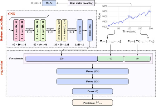
Now we discuss the structure of the CNN in our HDNN model. Inspired by the art-of-the-state VGG16 network (Zhang et al., 2016), the CNN comprises six conv2D (2 D convolution) layers and a fully connected dense layer, detailed as follows:

• Similar to VGG16 (Simonyan & Zisserman, 2015), we use the two stacked $3\times 3$ conv2D layers with a stride of one throughout the whole neural network rather than relatively large receptive fields in the convolution layers. The advantage of such a network structure is that it needs fewer parameters but obtains more nonlinearity or discriminative ability than $5\times 5$ or $7\times 7$ conv2D layers.

• To extract the underlying temporal feature from GAF images, we configure three groups of two stacked conv2D layers with 32, 64, 128 channels, as shown in different colours in Figure 2.

• To avoid model overfitting, we implement the Dropout layer after the convolution layers. It offers remarkably effective regularisation to improve the generalisation ability in deep neural networks.

• Moreover, we use ReLU for the activation function in each layer. Since ReLU has a simple formula $\text{max}(0,x),$ it obtains a more efficient gradient computation than the sigmoid or tanh function. Additionally, it reduces the vanishing gradient issue during the training procedure.

• Finally, we use a flatten layer to convert the output of the conv2D layers into a single long feature vector. With the flattening vector, we further connect it to a dense layer to perform dimensionality reduction. In other words, we put all the high-dimensional tensors together in one line and make connections with the dense layer.

After obtaining the feature vector from the dense layer in the CNN, we combine it with the historical time-series ${\mathit{R}}_t$ and ${\mathit{V}}_t$ via a concatenation operation. Then, the concatenated vector is fed as the input of the follow-up network for volatility forecasting. Here, we utilise three fully connected dense layers to implement the regression task: the first two have 128 channels with the ReLU activation function, and the third performs volatility forecasting with one output channel. The configuration of these dense layers is the same in all networks.

Once the HDNN model is built, we should design a criterion to validate its forecasting ability to guide the model optimisation. It is worth noting that the loss function plays an essential role during the model learning phase, which measures how good the prediction is. Namely, we estimate the model performance iteratively via the loss function and then update the parameters to reduce errors on the subsequent evaluation. In our model learning, we adopt the mean square error (MSE) or least square as the loss function (12) $$\mathit{MSE}=\frac{1}{m}\sum _{i=1}^m{\left(R{V}_i-\widehat{R{V}_i}\right)}^2$$(12) where $\widehat{R{V}_i}$ is the volatility forecast, $R{V}_i$ is the ground-truth volatility, and $m$ is the scale of the dataset. MSE is the average of the squared differences between the predicted $\widehat{R{V}_i}$ and actual $R{V}_i,$ which is one of the best measures for volatility.

Remark 2.

Different from most existing volatility forecasting methods, our HDNN can automatically learn the volatility-related temporal embedding via a convolution neural network. Specically, it enjoys the following attractive features: (1) Rather than learning from the time-series data directly, HDNN utilises an elegant strategy to encode one-dimensional time-series data as two-dimensional GAF images. These encoding images can preserve the temporal relationship between successive time intervals. (2) HDNN is an end-to-end learning model for volatility forecasting. There is no need to construct or select features manually. That is, it can learn the temporal feature mapping and the volatility forecasting task simultaneously. (3) The network architecture of HDNN consists of feature embedding and regression. The feature embedding component explores the volatility-related embedding space from GAF images via CNN. Meanwhile, the regression component takes the embedding vectors of the time-series data to perform volatility forecasting tasks.

4. Experimental setting

To demonstrate the validity of our HDNN model, we investigate its performance on both synthetic and real-world time-series datasets. The synthetic datasets are generated by the geometric Brownian motion (GBM) process, while the real-world datasets are collected from five Stock Index datasets. The implementations are carried out on a Linux Centos workstation using Python 3.8 with an Intel i9-10090k processor (3.7 GHz) and 128 GB random-access memory (RAM).

4.1. Baselines

Our experiments focus on comparisons between the proposed HDNN and five time-series forecasting methods, including GARCH, EGARCH, linear kernel SVR, RBF kernel SVR and NN, detailed as follows:

• GARCH (Bollerslev, 1986) and EGARCH (Nelson, 1991) are popular volatility methods that use observations of returns to model volatility shocks. Here, we utilise the ‘ARCH’ Python library to train both GARCH and EGARCH in our experiments. The optimal lag parameters ($p$ and $q$) in GARCH and EGARCH are chosen from $\left\{1,2,\dots ,10\right\}$ according to the Bayesian Information Criteria (BIC).

• SVR (Mishra & Padhy, 2019) is the regression version of SVM, which is a preeminent maximum-margin learning paradigm for data mining. The structural risk minimisation principle gives SVR an excellent generalisation ability. We consider the linear SVR (SVR_lin) and the RBF nonlinear SVR (SVR_rbf) for comparison in the experiments. Moreover, we utilise the ‘scikit-learn’ Python library to train these SVR models. The optimal parameters ($C$ for both SVR models and $\sigma$ for RBF kernel) are chosen from $\left\{2^{-6},2^{-5},\dots ,2^5,2^6\right\}$ according to the cross-validation method.

• Neural Network (NN) (LeCun et al., 2015), is a well-known mathematical model that uses learning algorithms to explore the underlying pattern among data. It employs a series of hidden neurons to approximate the complex relationships between inputs and outputs. For a better comparison, the structure of the baseline NN consists of three dense layers with the same setting as the regression part of the HDNN. The combination vector of the historical log returns and realised volatility time-series is the input of the NN. We utilise the ‘PyTorch’ deep learning Python library with CUDA 10.2 to develop both the NN and our HDNN. The Adam optimiser is used to train these models on an NVIDIA GPU (Quadro RTX 8000). Moreover, the learning rate is chosen from the set $\left\{0.0001,0.005,0.001,0.005\right\}.$

4.2. Performance criteria

In this subsection, we describe the criteria used to evaluate the performance of these volatility forecasting models. Without loss of generality, let $m$ be the number of samples, $\widehat{R{V}_i}$ be the volatility forecast, $R{V}_i$ be the ground-truth volatility, and $\overline{RV}=\frac{1}{m}{\sum }_{i=1}^{m}R{V}_i$ be the average value of the series $\left\{R{V}_1,R{V}_2,\dots ,R{V}_m\right\}.$ Then we use the following criteria (Davidovic, 2021; Liu, 2019; Wu et al., 2021; Yang et al., 2020) for model evaluation.

• RMSE: The mean squared error (MSE) is a risk metric corresponding to the expected value of the squared error, defined as (13) $$\mathit{RMSE}=\sqrt{\frac{1}{m}\sum _{i=1}^m{\left(R{V}_i-\widehat{R{V}_i}\right)}^2}$$(13)

• MAD: The mean absolute deviation (MAD) is a risk metric corresponding to the expected value of the absolute error, defined as (14) $$\mathit{MAD}=\frac{1}{m}\sum _{i=1}^m|R{V}_i-\widehat{R{V}_i}|$$(14)

• MedAE: The median absolute error (MedAE) is calculated by taking the median of all absolute differences between the ground truth and the prediction, defined as (15) $$\mathit{MedAE}=\mathrm{median}\left(\left|R{V}_1-\widehat{R{V}_1}\left|,\dots ,\right|R{V}_m-\widehat{R{V}_m}\right|\right)$$(15)

• MAPE: The mean absolute percentage error (MAPE) is the mean or average of the absolute percentage errors of forecasts, defined as (16) $$\mathit{MAPE}=\frac{100}{m}\sum _{i=1}^m\frac{\left|R{V}_i-\widehat{R{V}_i}\right|}{R{V}_i}$$(16)

• R²: The coefficient of determination R² is a statistical measure that represents the proportion of the variance for a dependent variable, defined as (17) $$R^2=1-\frac{{\sum }_{i=1}^m\left|R{V}_i-\widehat{R{V}_i}\right|}{{\sum }_{i=1}^m\left|R{V}_i-\overline{RV}\right|}$$(17)

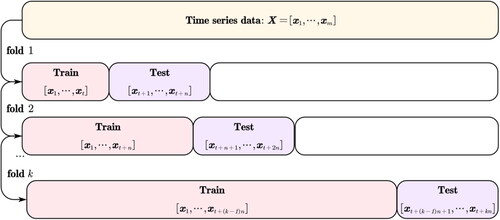
4.3. Time-series cross-validation for volatility forecasting

For the time-series learning tasks, the traditional cross-validation strategy becomes invalid. Namely, we cannot split training and validating sets in the random sense for the time-series forecasting. The reason is that such a random instance selection mechanism will cause discontinuity and break down the temporal relationship within the series. It makes no sense to forecast the past using future-looking data. Thus, we must avoid choosing future-looking data in the training set during model learning. In short, we should preserve the temporal dependency within the training and validating dataset.

To address the above issue, we utilise cross-validation on a rolling basis (Bergmeir & Benítez, 2012) for our forecasting learning task, as shown in Figure 3. Specifically, we begin with a small subset of series data from the start to the $t$ timestamp for training and forecast the follow-up future data with a length of $t+n.$ Then, we evaluate the forecasting performance with the criteria in Section 4.2. Subsequently, we expand the training set to the $t+n$ timestamp with the last forecasted data and forecast the future segment with $n$ length. The process moves the forecasted segment successively until it hits the end of the instances.

Figure 3. The procedure of time-series cross-validation on rolling windows.

Source: The authors’ illustration.

5. Experimental analysis

5.1. Results of the synthetic GBM time-series datasets

To demonstrate the effectiveness of our HDNN model, in this subsection, we perform comparisons on the synthetic time-series datasets generated by the geometric Brownian motion (GBM) process (Chen & Tsai, 2020). GBM is a powerful mathematical finance tool to model stock prices, similar to the famous Black-Scholes pricing model. It describes the pricing model as a continuous-time stochastic process, in which the logarithm of price $p_t$ over time obeys a Brownian diffusion process: (18) $$d{p}_t=r{p}_{t}dt+\sigma p_{t}d{w}_t$$(18) where $r$ is the risk-free rate, $\sigma$ is the constant volatility for the pricing process, and the random variable $w_t\sim \mathcal{N}(0,{\sigma }^{2}t).$ For an initial price $p_0,$ Equation (18)(18) $$d{p}_t=r{p}_{t}dt+\sigma p_{t}d{w}_t$$(18) has an analytic solution: (19) $$p_t=p_0\hspace{0.17em}\text{exp}\hspace{0.17em}\left(r-\frac{{\sigma }^2}{2}\right)t+\sigma w_t$$(19)

Following the GBM process in Equation (19)(19) $$p_t=p_0\hspace{0.17em}\text{exp}\hspace{0.17em}\left(r-\frac{{\sigma }^2}{2}\right)t+\sigma w_t$$(19) , we generate four pricing time-series with different levels, i.e., $\sigma =\left\{0.05,0.1,0.15,0.2\right\}.$ Each pricing series consists of 1000 samples with a random initial value $p_0,$ as illustrated in Figure 4. For simplicity, we use TypeA ∼ TypeD to notate them. Figure 4 shows that TypeA ∼ TypeD have diverse volatilities and tendencies, which can reflect different market situations. Table 1 summarises the statistics of volatility on these datasets.

Figure 4. The illustration of four types of GBM time-series datasets.

Source: The authors’ illustration.

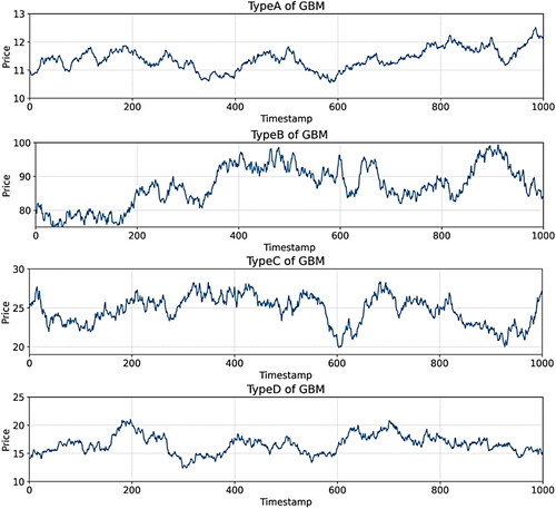
Table 1. The statistics of realised volatility for the four GBM time-series datasets.

Datasets	Mean	Std	Skewness	Kurtosis
TypeA	0.4558	0.1618	0.3591	0.5102
TypeB	0.9501	0.3496	0.4871	−0.0607
TypeC	1.4351	0.5517	0.3453	0.3326
TypeD	1.8372	0.6412	0.2531	−0.2236

Source: The authors’ illustration.

In our experiments, we train and test each forecasting model via the five-fold time-series cross-validation executions. Table 2 records the mean and std results of six regressors on each GBM time-series dataset in terms of the five metrics. The entries in table with the best performance (the lowest RMSE, MAD, MedAD and MAPE, and the highest R²) are highlighted in bold. Each entry in Table 2 has two parts: the first denotes the mean value of the cross-validation results, and the second stands for plus or minus the standard deviation. From Table 2, we can obtain the following:

Table 2. The forecasting results of each regressor on the four GBM time-series datasets, in terms of the five metrics.

Datasets	Regressors	RMSE↓	MAD↓	MedAD↓	MAPE↓	R^2↑
TypeA	GARCH	0.164 ± 0.020	0.130 ± 0.017	0.108 ± 0.020	0.422 ± 0.098	0.017 ± 0.048
	EGARCH	0.162 ± 0.015	0.128 ± 0.013	0.107 ± 0.017	0.417 ± 0.098	0.033 ± 0.088
	SVR_lin	0.126 ± 0.026	0.096 ± 0.022	0.074 ± 0.026	0.270 ± 0.076	0.392 ± 0.176
	SVR_rbf	0.118 ± 0.021	0.089 ± 0.018	0.070 ± 0.021	0.241 ± 0.057	0.409 ± 0.196
	NN	0.119 ± 0.021	0.089 ± 0.019	0.065 ± 0.016	0.251 ± 0.072	0.447 ± 0.194
	HDNN	0.112 ± 0.009	0.083 ± 0.007	0.061 ± 0.004	0.228 ± 0.035	0.517 ± 0.087
TypeB	GARCH	0.341 ± 0.033	0.284 ± 0.029	0.254 ± 0.025	0.397 ± 0.067	0.057 ± 0.082
	EGARCH	0.327 ± 0.025	0.272 ± 0.020	0.246 ± 0.014	0.384 ± 0.065	0.089 ± 0.145
	SVM_lin	0.254 ± 0.077	0.199 ± 0.068	0.162 ± 0.075	0.264 ± 0.117	0.392 ± 0.294
	SVM_rbf	0.243 ± 0.059	0.191 ± 0.058	0.153 ± 0.070	0.252 ± 0.092	0.443 ± 0.239
	NN	0.234 ± 0.035	0.182 ± 0.036	0.143 ± 0.038	0.241 ± 0.069	0.490 ± 0.133
	HDNN	0.220 ± 0.010	0.167 ± 0.008	0.125 ± 0.005	0.215 ± 0.025	0.550 ± 0.090
TypeC	GARCH	0.532 ± 0.066	0.440 ± 0.061	0.386 ± 0.088	0.419 ± 0.049	0.047 ± 0.048
	EGARCH	0.524 ± 0.065	0.433 ± 0.060	0.379 ± 0.083	0.415 ± 0.050	0.076 ± 0.051
	SVM_lin	0.382 ± 0.035	0.285 ± 0.034	0.225 ± 0.047	0.251 ± 0.042	0.482 ± 0.218
	SVM_rbf	0.367 ± 0.037	0.277 ± 0.038	0.213 ± 0.049	0.246 ± 0.055	0.504 ± 0.232
	NN	0.362 ± 0.031	0.273 ± 0.030	0.211 ± 0.032	0.241 ± 0.045	0.521 ± 0.199
	HDNN	0.349 ± 0.016	0.260 ± 0.009	0.197 ± 0.010	0.224 ± 0.009	0.570 ± 0.090
TypeD	GARCH	0.615 ± 0.037	0.501 ± 0.026	0.458 ± 0.030	0.371 ± 0.051	0.052 ± 0.059
	EGARCH	0.627 ± 0.026	0.512 ± 0.017	0.451 ± 0.021	0.380 ± 0.046	0.014 ± 0.052
	SVM_lin	0.473 ± 0.145	0.360 ± 0.124	0.272 ± 0.124	0.236 ± 0.064	0.416 ± 0.345
	SVM_rbf	0.465 ± 0.113	0.352 ± 0.090	0.269 ± 0.087	0.229 ± 0.037	0.443 ± 0.236
	NN	0.433 ± 0.053	0.330 ± 0.048	0.257 ± 0.057	0.222 ± 0.027	0.528 ± 0.088
	HDNN	0.422 ± 0.034	0.315 ± 0.022	0.234 ± 0.034	0.211 ± 0.017	0.554 ± 0.049

Source: The authors’ illustration.

• Our HDNN model yields better generalisation capability than other models in all cases. Specifically, HDNN exhibits the smallest RMSE, MAD, MedAD and MAPE with the largest R² among these methods. It confirms the effectiveness of our HDNN in forecasting time-series data with different volatility levels.

• The comparison results between HDNN and NN show that the feature embedding component helps HDNN construct the informative temporal embedding space. As a result, it can better understand the volatility and tendency within the time-series data.

• The machine learning models (HDNN, NN, and SVR) outperform the traditional ARCH based methods (GARCH and EGARCH), with a lower forecasting error and variance in most cases. GARCH and EGARCH formulate the volatility in the linear sense, which may not be suitable for high volatility cases.

5.2. Results on the real-world Stock Index datasets

In this subsection, we apply our HDNN to forecast the volatility of five 5-minute high-frequency real-world Stock Index datasets. These datasets¹ come from the CSI300 Index (000300.SS), SSE50 Index (000016.SS), ChiNext Index (399006.SZ), S&P 500 Index (.SPX), and NASDAQ Composite (.IXIC), described as follows:

• The CSI300 Index is a capitalisation-weighted stock market index designed to reflect the performance of the top 300 A-shares on the Shanghai Stock Exchange (SSE) and the Shenzhen Stock Exchange (SZSE). It consists of the 300 constituent stocks with the largest market capitalisation and liquidity from the entire universe of A-share enterprises in China.

• The SSE50 Index consists of the 50 most representative A-shares from the SSE by the scientific and objective method. It aims to reflect the complete picture of those excellent quality enterprises, which have the most influence within SSE.

• The ChiNext Index is free-float capitalisation-weighted and comprises the 100 largest liquid A-shares listed on the ChiNext Market of SZSE. As the benchmark index of the ChiNext Market, the ChiNext Index aims to reflect the performance of innovative businesses and emerging industries.

• The S&P 500 Index is a stock market index tracking the performance of 500 large companies listed on stock exchanges in the United States. It is one of the most commonly followed equity indices.

• The NASDAQ Composite is a stock market index that includes almost all stocks listed on the NASDAQ stock exchange in the United States. The composition of the NASDAQ Composite is heavily weighted towards companies in the information technology sector.

Specifically, our experiments use the 5-minute high-frequency data of CSI300, SSE50, ChiNext, S&P 500, and NASDAQ observed in the last three years: 2019, 2020, and 2021, as shown in Figure 5. Firstly, we conduct an exploratory data analysis on the above index datasets to investigate their characteristics. Take CSI300 in 2020 for example. Figure 6 plots the corresponding intraday log returns (left) and realised volatility (right). Continuous fluctuations appear during different timeframes. Due to the effects of COVID-19, the fluctuations in the first half of 2020 are relatively large, while the fluctuations in the second half tend to be stable. This phenomenon indicates that the financial market is more sensitive to unpredictable events than other forecasting applications. Moreover, Table 3 summarises the statistics of realised volatility on these datasets.

Figure 5. The illustration of CSI300, SSE50, ChiNext, S&P 500, and NASDAQ datasets.

Source: The authors’ illustration.

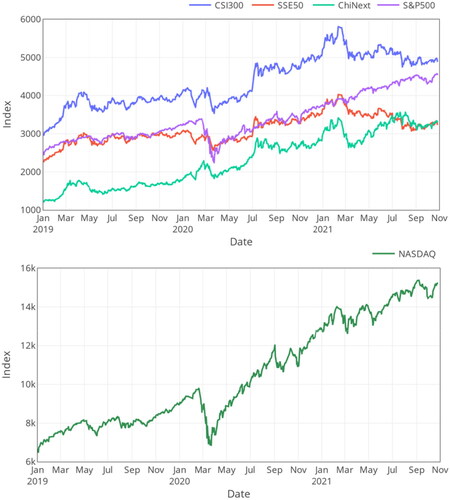
Figure 6. The log returns (left) and realized volatility (right) of CSI300 index in 2020.

Source: The authors’ illustration.

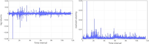
Table 3. The statistics of realized volatility for the five Stock Index datasets.

Datasets	Year	Samples	Mean	Std	Skewness	Kurtosis
CSI300 (000300.SS)	2019	11707	0.1226	0.1030	4.6032	36.6748
	2020	11664	0.1356	0.1371	11.9027	274.2992
	2021	9264	0.1354	0.0918	2.8142	14.2064
SSE50 (000016.SS)	2019	11707	0.1192	0.0995	4.2232	29.7014
	2020	11664	0.1299	0.1270	10.4634	222.4348
	2021	9264	0.1397	0.0913	2.4601	10.3207
ChiNext (399006.SZ)	2019	11707	0.1642	0.1204	3.9350	29.6242
	2020	11664	0.1905	0.1533	7.3723	120.1962
	2021	9264	0.2007	0.1360	2.5952	11.9347
S&P 500 (.SPX)	2019	11707	0.0711	0.0978	6.2247	52.4028
	2020	11664	0.1209	0.2046	7.2763	82.5521
	2021	9264	0.0692	0.0994	5.3037	35.2403
NASDAQ (.IXIC)	2019	11707	0.0745	0.1204	6.0673	49.0550
	2020	11664	0.1703	0.2541	4.8389	35.0700
	2021	9264	0.0707	0.1416	5.8012	42.4892

Source: The authors’ illustration.

To verify the forecasting ability of the models, we perform the five-fold time-series cross-validation on the above real-world Stock Index datasets. Figures 7–11 illustrate the box plot of the comparison results of each regressor in terms of RMSE, MAD, MedAD, MAPE and R². Box in these Figures records the metric score of the five-fold cross-validation for each regressor on each dataset, including the minimum score, first (lower) quartile, median, third (upper) quartile, and maximum score. The lower the RMSE, MAD, MedAD, and MAPE, the better performance of the regressor is; vice versa for R². Moreover, the larger the interquartile range in the box, the more the deviation of the regressor is. From Figures 7–11, we can obtain that:

Figure 7. The RMSE metric of regressors on the five Stock Index datasets.

Source: The authors’ illustration.

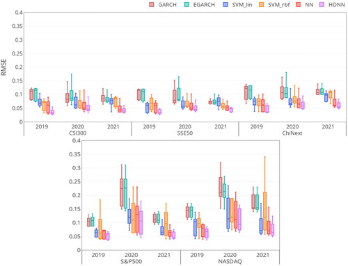
Figure 8. The MAD metric of regressors on the five Stock Index datasets.

Source: The authors’ illustration.

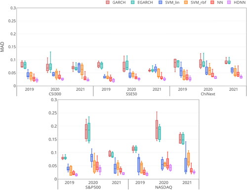
Figure 9. The MedAD metric of regressors on the five Stock Index datasets.

Source: The authors’ illustration.

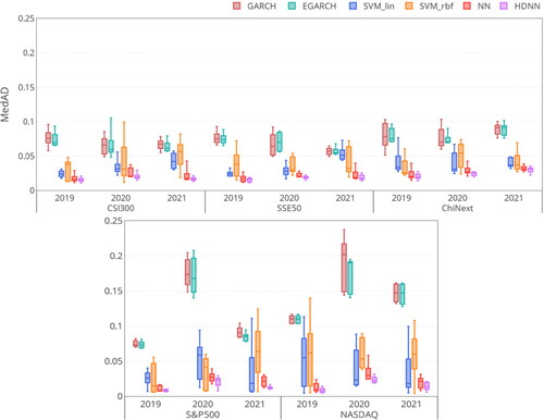
Figure 10. The MAPE metric of regressors on the five Stock Index datasets.

Source: The authors’ illustration.

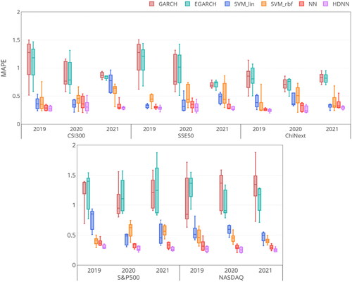
Figure 11. The R² metric of regressors on the five Stock Index datasets.

Source: The authors’ illustration.

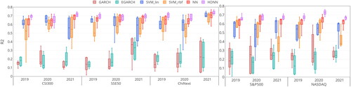
• HDNN performs fairly well and has a smaller RMSE, MAD, MedAD and MAPE with a larger R² on almost all datasets. It confirms the efficacy of the proposed HDNN on high-frequency time-series learning tasks.

• The prediction results of the HDNN, NN, and SVM are better than those of the statistical GARCH and EGARCH models. The reason is that GARCH and EGARCH only consider the linear structure of variance to model volatility, leading to less capability to track the complex high-frequency information.

• HDNN and NN outperform SVR in most cases. The structure of SVR can be seen as a single hidden layer shallow network, which is suitable for small sample tasks. For large-scale learning cases, the nonlinear multilayer network of HDNN and NN enjoys more capacity than SVR to exploit the high-frequency volatility trend.

• HDNN achieves better performance than NN. With the help of the time-series encoding framework, our HDNN can use the CNN to extract the underlying temporal embedding from the high-frequency time-series data. This strategy enables HDNN to learn more informative features for volatility, which helps improve forecasting performance.

To provide more statistical evidence (Hatamlou, 2013; Yu et al., 2017), we employ the Friedman test to verify whether there are significant differences between HDNN and the other regressors on the learning results in Figures 7–11. Tables 4–8 record the rank of regressors obtained via the Friedman test according to each metric. The results show that HDNN is ranked first in the whole situation, followed by NN successively.

Table 4. Rank and statistic of the Friedman test on the CSI300 dataset.

Metric	Regressors (Rank)						Statistic	p-value	Hypothesis
	GARCH	EGARCH	SVM_lin	SVM_rbf	NN	HDNN
RMSE	5.0666	5.0666	3.8000	3.6000	2.4666	1.0000	33.3428	4.08954E-10	reject
MAD	5.4000	5.4666	3.2666	3.0666	2.6666	1.1333	23.0962	6.5955E-9	reject
MedAD	5.4666	5.1333	3.2000	3.2666	2.5999	1.3333	32.0911	5.1398E-10	reject
MAPE	5.6000	5.2000	3.4000	2.9333	2.4666	1.4000	41.7945	1.0913E-10	reject
R^2	5.5333	5.2666	2.8000	3.6000	2.2666	1.5333	42.2500	1.0809E-10	reject

Source: The authors’ illustration.

Table 5. Rank and statistic of the Friedman test on the SSE50 dataset.

Metric	Regressors (Rank)						Statistic	p-value	Hypothesis
	GARCH	EGARCH	SVM_lin	SVM_rbf	NN	HDNN
RMSE	5.3333	5.1999	3.4333	3.6333	2.4000	1.0000	51.0120	6.0951E-11	reject
MAD	5.3666	5.2666	3.0000	3.5666	2.4000	1.4000	34.8047	2.9598E-10	reject
MedAD	5.2666	5.2666	3.4666	3.6000	2.2666	1.1333	45.4019	7.5646E-11	reject
MAPE	5.4000	5.3999	2.6000	3.7333	2.4000	1.4666	46.1801	7.7125E-11	reject
R^2	5.7333	5.2666	2.7333	3.6666	2.0666	1.5333	71.8644	4.7931E-11	reject

Source: The authors’ illustration.

Table 6. Rank and statistic of the Friedman test on the ChiNext dataset.

Metric	Regressors (Rank)						Statistic	p-value	Hypothesis
	GARCH	EGARCH	SVM_lin	SVM_rbf	NN	HDNN
RMSE	5.1333	5.4000	3.1333	4.0000	2.3333	1.0000	61.9297	4.2042E-11	reject
MAD	5.4000	5.4666	3.2666	3.0666	2.6666	1.1333	56.3125	5.0725E-11	reject
MedAD	5.6000	5.1999	3.4000	3.2000	2.3333	1.2666	51.3139	6.2281E-11	reject
MAPE	5.6666	5.2666	3.3333	2.8667	2.6000	1.2666	56.8547	5.3429E-11	reject
R^2	5.5333	5.4666	3.1333	3.2000	2.2666	1.4000	59.3045	6.8930E-11	reject

Source: The authors’ illustration.

Table 7. Rank and statistic of the Friedman test on the S&P 500 dataset.

Metric	Regressors (Rank)						Statistic	p-value	Hypothesis
	GARCH	EGARCH	SVM_lin	SVM_rbf	NN	HDNN
RMSE	5.2333	5.2333	3.2000	3.4999	2.6000	1.2333	51.6285	6.87707E-10	reject
MAD	5.6000	5.3999	2.8000	3.0000	2.6666	1.5333	57.0952	1.16210E-9	reject
MedAD	5.7333	5.0000	2.9333	3.0000	2.5666	1.7666	50.0761	1.37109E-9	reject
MAPE	5.5333	5.3999	3.2666	3.2666	2.2333	1.2999	61.2761	4.4418E-11	reject
R^2	5.1999	5.4666	3.4000	3.4666	2.3666	1.0999	59.1999	6.9053E-11	reject

Source: The authors’ illustration.

Table 8. Rank and statistic of the Friedman test on the NASDAQ dataset.

Metric	Regressors (Rank)						Statistic	p-value	Hypothesis
	GARCH	EGARCH	SVM_lin	SVM_rbf	NN	HDNN
RMSE	5.5333	5.0666	3.2666	3.8666	2.2666	1.0000	62.3523	3.72648E-11	reject
MAD	5.7666	5.2333	2.2666	3.2666	2.6666	1.7999	57.0095	1.14100E-9	reject
MedAD	5.6000	5.1333	2.6666	3.3333	2.7333	1.5333	32.0911	5.1398E-10	reject
MAPE	5.6666	5.3333	3.8000	3.0000	1.9333	1.2666	67.8761	4.5638E-11	reject
R^2	5.1666	5.7666	3.5333	3.3333	2.1666	1.0333	67.7428	4.1790E-11	reject

Source: The authors’ illustration.

Now, we calculate the ${\mathcal{X}}_F^2$ value for the Friedman test as follows: (20) $${\mathcal{X}}_F^2=\frac{12N}{k\left(k+1\right)}\left[\sum _{i=1}^k{r}_i^2-\frac{k{(k+1)}^2}{4}\right]$$(20) where $k$ is the number of regressors, and $r_i$ is the rank on the $N$ datasets for the i-th regressor listed in Tables 4–8. In our experiments, $k=6$ and $N=15$ (3 years with the five-fold time-series cross-validation, i.e., $N=3\times 5$).

Let us consider, for example, the RMSE metric on CSI300. The term ${\sum }_{i=1}^k{r}_i^2$ is computed for the first line of Table 4: (21) $$\sum _{i=1}^k{r}_i^2=\left({5.0666}^2+{5.0666}^2+{3.8}^2+{3.6}^2+{2.4666}^2+{1.0}^2\right)\approx 85.8249$$(21)

Then, substituting $k=6,$ $N=15,$ and (21) into (20), we obtain (22) $${\mathcal{X}}_F^2=\frac{12\times 15}{6\left(6+1\right)}\left[85.8249-\frac{6{(6+1)}^2}{4}\right]=52.8213$$(22)

Based on the above Friedman statistic ${\mathcal{X}}_F^2=52.8213,$ we calculate the F-distribution statistic ${\mathcal{F}}_F$ with $(k-1,(k-1)(N-1))=(5,70)$ degrees of freedom (23) $${\mathcal{F}}_F=\frac{\left(N-1\right)\times {\mathcal{X}}_F^2}{N\left(k-1\right)-{\mathcal{X}}_F^2}=\frac{\left(15-1\right)\times 52.8213}{15\times \left(6-1\right)-52.8213}\approx 33.3428$$(23)

Similarly, we calculate the statistic ${\mathcal{F}}_F$ for the other cases, summarised in the ‘Statistic’ column of Tables 4–8. Additionally, the p-value is provided by the Friedman test. The significance level is set as 0.05. The results reject the null hypothesis (there is no significant difference among the compared regressors.) for these datasets. It indicates that our HDNN is statistically superior to the other forecasting models. Overall, the above results confirm the feasibility of HDNN.

6. Conclusion

Learning volatility from time-series data plays an essential role in making investment decisions for the financial market. This paper proposes a novel deep neural network model with temporal embedding for volatility forecasting, termed HDNN. The main characteristics of our HDNN are as follows:

1. An elegant time-series encoding strategy is introduced to transform one-dimensional time-series data into two-dimensional GAF images. These images can preserve the temporal relationship among the time-series data.

2. With the encoding GAF images, the follow-up CNN can automatically learn the volatility-related feature mappings, which is very challenging for traditional feature engineering methods. The feature embedding component can explore an underlying temporal embedding space from the GAF images via the elaborate CNN. The new representation vectors of the time-series data in the embedding space preserve the temporal information as much as possible.

3. HDNN is an end-to-end learning model for volatility forecasting. It can simultaneously carry out temporal feature learning (feature embedding component) and volatility forecasting tasks (regression component).

Note that most existing methods (Henrique et al., 2019; Wang et al., 2021) directly utilise the raw time-series data to build the volatility forecasting model. However, the raw time-series data cannot effectively express the volatility tendency. To address the above issue, our HDNN encodes one-dimensional time-series data as two-dimensional GAF images rather than directly learning from the raw time-series data. Then, the CNN constructs the most volatility-related features in the embedding space. Afterwards, the volatility-related features are used to train the forecasting regressor. Compared with the raw data, these features can better represent the time-series data with more helpful and pure information related to volatility.

Finally, the proposed HDNN model is compared with the state-of-the-art GARCH, EGACH, SVR, and NN models on the GBM synthetic dataset and the real-world high-frequency Stock Index datasets (CSI300, SSE50, ChiNext, S&P 500, and NASDAQ). The extensive results confirm that the HDNN remarkably improves the forecasting ability. Furthermore, the Friedman test results indicate that HDNN is statistically superior to the other forecasting models.

Our future research works will extend the HDNN to examine more high-frequency volatility forecasting situations, such as 1-minute intervals or tick levels. Moreover, stock picking based on regularities in the time series is one of the most valuable topics in the financial industry (Barucci et al., 2021). However, selecting high-quality stocks is very challenging. Various machine learning techniques have been employed for this task. Another future work is applying our HDNN to build a trading strategy algorithm based on real-time intraday time-series data.

Disclosure statement

No potential conflict of interest was reported by the author(s).

Additional information

Funding

This work is supported by the National Natural Science Foundation of China (Nos. 61603338, 11871183, 61866010, and 11426202), the Natural Science Foundation of Zhejiang Province (Nos. LY21F030013), the Natural Science Foundation of China Hainan Province (Nos. 120RC449), the Scientific Research Foundation of Hainan University (Nos. kyqd(sk)1804).

Notes

1 CSI300, SSE50, and ChiNext datasets were collected from Ricequant (www.ricequant.com). S&P 500 and NASDAQ datasets were acquired from Alpha Vantage (www.alphavantage.co). All datasets are available under an academic licence.

References

- Barra, S., Carta, S. M., Corriga, A., Podda, A. S., & Recupero, D. R. (2020). Deep learning and time series-to-image encoding for financial forecasting. IEEE/CAA Journal of Automatica Sinica, 7(3), 683–692. https://doi.org/10.1109/JAS.2020.1003132
- Barucci, E., Bonollo, M., Poli, F., & Rroji, E. (2021). A machine learning algorithm for stock picking built on information based outliers. Expert Systems with Applications, 184, 115497. https://doi.org/10.1016/j.eswa.2021.115497
- Bauwens, L., Hafner, C. M., & Rombouts, J. V. K. (2007). Multivariate mixed normal conditional heteroskedasticity. Computational Statistics & Data Analysis, 51(7), 3551–3566. https://doi.org/10.1016/j.csda.2006.10.012
- Bergmeir, C., & Benítez, J. M. (2012). On the use of cross-validation for time series predictor evaluation. Information Sciences, 191, 192–213. https://doi.org/10.1016/j.ins.2011.12.028
- Bollerslev, T. (1986). Generalized autoregressive conditional heteroskedasticity. Journal of Econometrics, 31(3), 307–327. https://doi.org/10.1016/0304-4076(86)90063-1
- Chen, J., & Tsai, Y. (2020). Encoding candlesticks as images for pattern classification using convolutional neural networks. Financial Innovation, 6(1), 26–33. https://doi.org/10.1186/s40854-020-00187-0
- Davidovic, M. (2021). From pandemic to financial contagion: High-frequency risk metrics and Bayesian volatility analysis. Finance Research Letters, 42, 101913. https://doi.org/10.1016/j.frl.2020.101913
- Dvorsky, J., Belas, J., Gavurova, B., & Brabenec, T. (2021). Business risk management in the context of small and medium-sized enterprises. Economic Research-Ekonomska Istraživanja, 34(1), 1690–1708. https://doi.org/10.1080/1331677X.2020.1844588
- Ecer, F. (2013). Comparing the bank failure prediction performance of neural networks and support vector machines: The Turkish case. Economic Research-Ekonomska Istraživanja, 26(3), 81–98. https://doi.org/10.1080/1331677X.2013.11517623
- Eduardo, R., Pablo, J. A., & José, J. N. (2019). Forecasting volatility with a stacked model based on a hybridized Artificial Neural Network. Expert Systems with Applications, 129, 1–9.
- Engle, R. (2002). Dynamic conditional correlation: A simple class of multivariate generalized autoregressive conditional heteroskedasticity models. Journal of Business & Economic Statistics, 20(3), 339–350. https://doi.org/10.1198/073500102288618487
- Engle, R. F. (1982). Autoregressive conditional heteroscedasticity with estimates of the variance of United Kingdom inflation. Econometrica, 50(4), 987–1007. ), https://doi.org/10.2307/1912773
- Gabriel, T. R., André, A. P. S., Viviana, C. M., & Leandro, D. S. C. (2021). Novel hybrid model based on echo state neural network applied to the prediction of stock price return volatility. Expert Systems with Applications, 184, 115490.
- Ge, W., Lalbakhsh, P., Isai, L., Lenskiy, A., & Suominen, H. (2023). Neural Network-Based financial volatility forecasting: A systematic review. ACM Computing Surveys, 55(1), 1–40. https://doi.org/10.1145/3483596
- Hajizadeh, E., Seifi, A., Fazel Zarandi, M. H., & Turksen, I. B. (2012). A hybrid modeling approach for forecasting the volatility of S&P 500 index return. Expert Systems with Applications, 39(1), 431–436. https://doi.org/10.1016/j.eswa.2011.07.033
- Hatamlou, A. (2013). Black hole: A new heuristic optimization approach for data clustering. Information Sciences, 222, 175–184. https://doi.org/10.1016/j.ins.2012.08.023
- Henrique, B. M., Sobreiro, V. A., & Kimura, H. (2019). Literature review: Machine learning techniques applied to financial market prediction. Expert Systems with Applications, 124, 226–251. https://doi.org/10.1016/j.eswa.2019.01.012
- Khan, F., Rehman, S., Khan, H., & Xu, T. (2016). Pricing of risk and volatility dynamics on an emerging stock market: Evidence from both aggregate and disaggregate data. Economic Research-Ekonomska Istraživanja, 29(1), 799–815. https://doi.org/10.1080/1331677X.2016.1197554
- Kim, J., Kim, D. H., & Jung, H. (2021). Applications of machine learning for corporate bond yield spread forecasting. The North American Journal of Economics and Finance, 58, 101540. https://doi.org/10.1016/j.najef.2021.101540
- Kim, D., Yoon, J., & Park, C. (2021). Pricing external barrier options under a stochastic volatility model. Journal of Computational and Applied Mathematics, 394, 113555. https://doi.org/10.1016/j.cam.2021.113555
- Lampariello, L., Neumann, C., Ricci, J. M., Sagratella, S., & Stein, O. (2021). Equilibrium selection for multi-portfolio optimization. European Journal of Operational Research, 295(1), 363–373. https://doi.org/10.1016/j.ejor.2021.02.033
- LeCun, Y., Bengio, Y., & Hinton, G. (2015). Deep learning. Nature, 521(7553), 436–444. [Database] https://doi.org/10.1038/nature14539
- Lee, S. W., & Kim, H. Y. (2020). Stock market forecasting with super-high dimensional time-series data using ConvLSTM, trend sampling, and specialized data augmentation. Expert Systems with Applications, 161, 113704. https://doi.org/10.1016/j.eswa.2020.113704
- Liu, Y. (2019). Novel volatility forecasting using deep learning-long short term memory recurrent neural networks. Expert Systems with Applications, 132, 99–109. https://doi.org/10.1016/j.eswa.2019.04.038
- Li, T., Zhang, Y., & Wang, T. (2021). SRPM-CNN: A combined model based on slide relative position matrix and CNN for time series classification. Complex & Intelligent Systems, 7(3), 1619–1631. https://doi.org/10.1007/s40747-021-00296-y
- Li, D., Zhang, X., Zhu, K., & Ling, S. (2018). The ZD-GARCH model: A new way to study heteroscedasticity. Journal of Econometrics, 202(1), 1–17. https://doi.org/10.1016/j.jeconom.2017.09.003
- Ma, Y., Han, R., & Wang, W. (2021). Portfolio optimization with return prediction using deep learning and machine learning. Expert Systems with Applications, 165, 113973. https://doi.org/10.1016/j.eswa.2020.113973
- Mishra, S., & Padhy, S. (2019). An efficient portfolio construction model using stock price predicted by support vector regression. The North American Journal of Economics and Finance, 50, 101027. https://doi.org/10.1016/j.najef.2019.101027
- Nayak, R. K., Mishra, D., & Rath, A. K. (2015). A Naïve SVM-KNN based stock market trend reversal analysis for Indian benchmark indices. Applied Soft Computing, 35, 670–680. https://doi.org/10.1016/j.asoc.2015.06.040
- Nelson, D. B. (1991). Conditional heteroskedasticity in asset returns: A new approach. Econometrica, 59(2), 347–370. https://doi.org/10.2307/2938260
- Paolella, M. S., Polak, P., & Walker, P. S. (2019). Regime switching dynamic correlations for asymmetric and fat-tailed conditional returns. Journal of Econometrics, 213(2), 493–515. https://doi.org/10.1016/j.jeconom.2019.07.002
- Poon, S., & Granger, C. (2005). Practical issues in forecasting volatility. Financial Analysts Journal, 1(61), 45–56.
- Sezer, O. B., Gudelek, M. U., & Ozbayoglu, A. M. (2020). Financial time series forecasting with deep learning: A systematic literature review: 2005-2019. Applied Soft Computing, 90, 106181. https://doi.org/10.1016/j.asoc.2020.106181
- Shin, D. W. (2018). Forecasting realized volatility: A review. Journal of the Korean Statistical Society, 47(4), 395–404. https://doi.org/10.1016/j.jkss.2018.08.002
- Simonyan, K., & Zisserman, A. (2015). Very deep convolutional networks for large-scale image recognition. 3rd International Conference on Learning Representations, USA, San Diego, 1–10.
- Takahashi, M., Watanabe, T., & Omori, Y. (2021). Forecasting daily volatility of stock price index using daily returns and realized volatility. Econometrics and Statistics, preprint, 1–20.
- Vychytilová, J., Pavelková, D., Pham, H., & Urbánek, T. (2019). Macroeconomic factors explaining stock volatility: Multi-country empirical evidence from the auto industry. Economic Research-Ekonomska Istraživanja, 32(1), 3333–3347. https://doi.org/10.1080/1331677X.2019.1661003
- Wang, Z., & Oates, T. (2015). Imaging time-series to improve classification and imputation. 24th International Joint Conference on Artificial Intelligence, USA, Palo Alto, 3939–3945.
- Wang, Y., Xiang, Y., Lei, X., & Zhou, Y. (2021). Volatility analysis based on GARCH-type models: Evidence from the Chinese stock market. Economic Research-Ekonomska Istraživanja, preprint, 1–25.
- Wang, L., Xu, Y., & Salem, S. (2021). Theoretical and experimental evidence on stock market volatilities: A two-phase flow model. Economic Research-Ekonomska Istraživanja, preprint, 1–22.
- Wu, J. M., Li, Z., Herencsar, N., Vo, B., & Lin, J. C. (2021). A graph-based CNN-LSTM stock price prediction algorithm with leading indicators. Multimedia Systems, preprint, 1–20.
- Yang, R., Yu, L., Zhao, Y., Yu, H., Xu, G., Wu, Y., & Liu, Z. (2020). Big data analytics for financial market volatility forecast based on support vector machine. International Journal of Information Management, 50, 452–462. https://doi.org/10.1016/j.ijinfomgt.2019.05.027
- Yu, Z., Wang, Z., You, J., Zhang, J., Liu, J., Wong, H. S., & Han, G. (2017). A new kind of nonparametric test for statistical comparison of multiple classifiers over multiple datasets. IEEE Transactions on Cybernetics, 47(12), 4418–4431.
- Zhang, H., Nguyen, H., Vu, D., Bui, X., & Pradhan, B. (2021). Forecasting monthly copper price: A comparative study of various machine learning-based methods. Resources Policy, 73, 102189. https://doi.org/10.1016/j.resourpol.2021.102189
- Zhang, X., Zou, J., He, K., & Sun, J. (2016). Accelerating very deep convolutional networks for classification and detection. IEEE Transactions on Pattern Analysis and Machine Intelligence, 38(10), 1943–1955. https://doi.org/10.1109/TPAMI.2015.2502579