Towards self-recovering construction schedules: a new method for periodically updating project plans and optimizing recovery actions

ABSTRACT

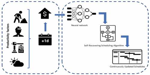
It is common for a construction schedule to deviate from its original-planned baseline, as uncertainty is inherent in all construction activities. Accordingly, planners are required to perform periodic schedule updates that learn from retrospective progress to more accurately schedule remaining activities and draw optimum recovery plans. This research proposes a method that utilizes a neural network regression model to forecast upcoming productivity rates based on retrospective progress and accordingly updates the schedule on a regular time interval with the required resource adjustments to meet the planned end date of the project with optimal cost. The method was tested on brickwork activities at a residential complex construction project in the UAE, using retrospective progress data of 1487 working days for 132 masons, and was found to be 98% accurate in predicting labor productivity, which was thus used as a basis to draw schedule recovery plans according to the proposed framework. In essence, this research provides a platform toward an automated self-recovering scheduling system, which serves construction managers in proactively preventing potential schedule deficiencies.

Graphical abstract

KEYWORDS:

• Productivity
• delay recovery
• fast tracking
• activity crashing
• neural network

1. Introduction

Construction project scheduling systems are currently based on an initial baseline plan and a limited number of recovery plans, which are made when the project’s baseline plan becomes unrealistic and far from the real progress at site. A recovery plan is a new plan for the project that starts from the current actual status of the project with one of the suggested strategies to recover the delay and finish the project on time with the least possible additional cost to recover the delay (Guida and Sacco 2019). Building a recovery plan goes through a long process. It is built by the contractor’s planning engineer and revised by the consultant, which is further approved by the client as the new project plan. Unfortunately, recovery plans usually yield with enormous actions that are expensive because it either adds resources to accomplish the remaining activities with significantly more compressed duration than what is in the baseline plan or divides the remaining work into more subcontractors to do the work in parallel which decreases the profit share (Martens and Vanhoucke 2019).

One of the most widespread recovery plan strategies is Activity Crashing. It involves loading the critical activities with more resources before reaching the maximum applicable resource load, which is usually due to limited working space, that is when we move or add resources to the next activity and so on (Hady, Al-Kindi, and Mahmoud 2020). Another strategy is Fast Tracking which is the execution of activities in parallel. This strategy requires assigning multiple subcontractors for the same type of activities in the project. It needs advanced management skills and hard efforts by the management team due to the risk of losing the sequence of activities, giving special attention to activity interdependencies. Moreover, additional cost applies on the main contractor due to commencing new contracts with sub-contractors who get a proportion of the originally assigned overhead (Ballesteros-Pérez, Elamrousy, and González-Cruz 2019).

The above-mentioned strategies are highly expensive with respect to cost and labor. For example, fast tracking requires the manager to start new deals under compressed conditions, which imposes taking costly decisions in order to divide the work on multiple subcontractors and start the work in parallel. On the other hand, activity crashing adds to the overall project cost and might cause saturated project conditions where the supervision staff might be insufficient to provide good quality.

The objective of this research is to propose a new periodically modified scheduling system based on proactive data reported from the site on a regular basis (e.g., weekly, daily) which includes the actual productivity of the crew and the current delay of the project. After each report, a neural network predicts the future productivity rates, which provides dynamism for the system. Then, the remaining activities are modified according to the predicted productivity rates. If the project is found to be behind schedule in the modified schedule, then the system enters into an optimization algorithm. In this algorithm, different recovery strategies, namely, activity crashing, fast tracking, and do nothing, are separately considered, and the best alternative is chosen.

The major task of the system is the automated process of continuously changing the planned duration, resource load, and/or the relationships of activities based on the results of the current and historical data of the project, which represents a starting point toward a bigger research that focuses on forming lean construction practice. This research also aims to change the role of the construction program in the project from monitoring to planning, which currently depends on the manual engineer’s modifications. The periodic mini recovery actions do not only minimize the cost of the delay recovery but also provide active contribution in the project time and cost management.

2. Literature review

2.1. Labor productivity factors and productivity prediction models

A labor productivity prediction model based on multilayer feedforward neural network (FFNN) with back-propagation learning algorithm was developed to predict the productivity of a concrete work of two power plant construction projects in Iran. The two major techniques “early stopping” and “Bayesian regularization” used to prevent data overfitting and to provide generalized networks were compared. It was concluded that the generalization performance of Bayesian regularization is better than that of early stopping. They also performed a sensitivity analysis of factors affecting productivity and found that labor qualification, decision-making quality, motivation, site layout organization, and planning are the most significant factors affecting productivity (Heravi and Eslamdoost 2015). A comparison study between FFNN and radial basis neural network (RBNN) models while analyzing the factors affecting productivity of masonry crew was conducted. The models were evaluated using both mean absolute percentage error (MAPE) and correlation oefficient (R). Based on the MAPE evaluation of model performance, RBNN was found to be more effective than FFNN, although both slightly overestimate the productivity, yet both techniques were successful in predicting construction productivity (Gerek et al. 2015).

Based on a regression model, the significant factors affecting labor productivity of reinforced concrete construction were found to be those related to workers (such as experience, health, motivation), work characteristics (such as work method, prefabrication, accessibility), work technologies (such as information technology, work continuity, and rework), and work management (which includes safety, planning, management system, and manager capabilities) (Jang et al. 2011).

Umit Dikmen and Sonmez (2011) developed an Artificial Neural Network (ANN) learning model to predict the needed man-hours for reinforced concrete formwork. They tested it with two case studies, and the results were considerably close to the actual field data, despite the fact that the model had a limited number of parameters, including building size, weather conditions, and working heights. According to an on-site questionnaire conducted with labors and mid level project personnel in a Chilean construction company, equipment, materials, and rework are the most significant factors affecting labor productivity (Rivas et al. 2011). A marble flooring productivity estimation model using ANN based on 10 factors affecting productivity and using data from different types of projects was developed. Their model performance was measured using four statistical measures, concluding high accuracy degree of the model, which was sufficiently attained using only one ANN hidden layer of one node in addition to the input and output layers. It was found that the most influencing factors affecting productivity are age, experience, and number of assisting labors. A statistic-based analysis of the same marble flooring dataset using multivariable linear regression technique was implemented to compare the results of MLR and ANN techniques and found that both produce significantly high accuracy measures with slightly higher values for the linear regression model that fits these specific marble flooring data better (Al-Zwainy, Rasheed, and Ibraheem 2012).

Project managers need to identify and evaluate factors affecting labor construction productivity to increase productivity in construction and thus avoid cost and schedule overruns. Considerable costs can be saved if productivity is improved because the same work can be done with less manpower, thus reducing overall labor cost. Productivity factors are classified into various groups. Different authors suggest different ways to categorize productivity factors as seen in the literature review. Hence, considering all the categories, productivity factors can be broadly classified as shown in Figure 1.

Figure 1. Classification of productivity factors.

The productivity factors as mentioned contribute to the productivity rates of each labor working in a project. Most of the time, the work will not progress according to the schedule due to various reasons. In such cases, appropriate recovery plans can be adopted to overcome the delay and ultimately meet the actual schedule of the project.

2.2. Project crashing techniques

The major techniques adopted to overcome the delay and to restructure the future activities to comply with the actual schedules are “activity crashing” and “fast tracking.” After it is found that the progress update is behind schedule, the contractor can either increase the manpower (activity crashing), do activities in parallel (fast tracking), or can even “do nothing” in response to the delay (Ballesteros-Pérez, Elamrousy, and González-Cruz 2019). The cost of each recovery option varies according to the project.

Activity crashing starts by filtering the longest path to perform the activity crashing, and then the model computes the compressed duration of the first activity, required to recover the delay, and also the required increase in crew size. The constraints on the maximum crew size are workspace limitations and activity-specific conditions. When the workspace limit of applicable manpower is exceeded, overtime working is a considerable option if applicable. The total cost of activity crashing is calculated by summing up the costs of increasing manpower and overtime working cost in all of the modified activities (Harun et al. 2020)

Fast tracking is the next option in which the activities are overlapped in a way that decreases the overall duration without affecting the sequence of work. The process of fast tracking starts from filtering the activities on the critical path; then, for the first activity, the system checks if overlapping is applicable and to which range; then, it compares the needed overlap with the applicable range; if it exceeds the maximum, the system enters a loop where it keeps performing overlapping on the subsequent activities until the delay duration is recovered. The system then reschedules the progress update and checks for other critical paths to be modified. Finally, the cost of fast tracking is computed by summing up the cost of assigning subcontractors or adding resources to do fast tracking (Sindhu et al. 2018)

“Do Nothing” is a recovery option adopted when the recovery cost is more than the delay cost. The delay cost includes delay penalty, cost related to the salary and resources, cost related to time in which the loss faced due to delay in the start of the next activity, administration cost, and so on (Lock 2017).

2.3. Project crashing models

Rescheduling the project activities of a delayed project to meet up with the originally planned completion date is a serious task for the project managers. Many efforts have been made in the past to develop several mathematical models, heuristic and metaheuristic algorithms in association with this challenge. A linear programming model was developed in which the cost, time, and quality of the project activities were taken into consideration for project crashing (Babu and Suresh 1996). Fuzzy theory and genetic algorithm were applied to develop models based on durations of activities (Leu, Chen, and Yang 2001).

Similarly, many other methods including and not limited to nonlinear model, stochastic models, two-stage robust scheduling algorithm, genetic and simulated annealing algorithm, multiobjective genetic algorithm, and deterministic particle swarm optimization algorithm have been developed for time–cost–quality tradeoff problems (Feylizadeh et al. 2018).

Different models have taken into consideration different parameters for dealing with the project delay including cost, time, etc. This study focuses on productivity of the labors to monitor the progress of the project. Productivity of labor is dependent on several factors as seen in the initial portion of this section. Hence, considering productivity for deciding on recovery actions can be beneficial since it reflects many other factors too. Neural network techniques have been previously applied to develop models to predict labor productivity as seen in the above section. However, this study aims to adopt neural network algorithm to develop a self-recovering schedule which facilitates updating the original schedule based on the actual productivity rate of the labors at the site. Thus, this paper represents a proactive approach rather than a reactive approach toward project delays. In addition, this study has selected brickwork activity to develop the model because it is one among the basic activities adopted in all types of construction projects.

3. Data collection and preprocessing

In order to measure the productivity of the labors, an activity needs to be selected. In this study, block work is selected as the activity to study productivity. The data associated with the block work in the construction of a villa complex project in Dubai, UAE, are utilized in this study. This activity was selected because it was comparatively easy to monitor this activity and data related to this activity were available. Labor details including their ID number, labor type, blocks per day (productivity of the labor), and the skill level of the labor and the supervisor are noted. These types of data are generally collected by supervisors in the industry. For model development, labor skill, supervisory skill, temperature, and humidity were selected as inputs since these factors were easy to monitor and in addition influenced productivity rate to a great extent as seen in the literature review. Productivity of the labor is measured by considering the number of blocks prepared by the labor per day. Labor skill is assumed to be the average productivity of the labor during the duration of the data collection. Supervisor skill corresponds to the average productivity of all labors supervised by a foreman. In addition, environmental conditions including temperature and humidity are included from the daily weather history. Skill levels, blocks per day, temperature, and humidity are normalized to prepare the database for model development. An example of the data collected is provided in Table 1.

Table 1. Representation of data collection.

Date	Villa No	Temperature	Humidity	Labor ID No	Labor type	^aBlocks per day	^bLabor skill	^cSupervisor skill
16 September 2017	235	39°C	63%	749	Mason	48	48.67	91.24

^aBlocks per day – It is the number of blocks prepared by the labor on that particular day

^bLabor skill – Average number of blocks prepared by the labor throughout the days of data collection

^cSupervisor skill- It is average number of blocks prepared by all the labors under the supervision of the foreman

Data corresponding to 3 weeks were monitored. Data from the first 2 weeks were used to train the model to predict the forthcoming productivity of the labors, and the data from week 3 were utilized to validate the results. One hundred and thirty-two masons are considered in this study. The difference in the actual value and the predicted value of the productivity rate was calculated to estimate the error in the model.

Each labor is under the supervision of a foreman who supervises the labor in his work. More than one labor can be under the supervision of a single foreman. Likewise, there are 17 supervisors in this project. Table 2 lists the number of labors under the supervision of each supervisor.

Table 2. Group details of the labors.

Group number	Supervisor Name	Number of labors (masons with their helpers) under the supervisor
1	S1	13
2	S2	5
3	S3	16
4	S4	8
5	S5	8
6	S6	7
7	S7	12
8	S8	7
9	S9	5
10	S10	6
11	S11	4
12	S12	15
13	S13	4
14	S14	5
15	S15	6
16	S16	5
17	S17	6

4. Research method

4.1. Neural network model

This model uses a machine learning algorithm composed of a multilayer FFNN with backpropagation learning algorithm to predict productivity rates of the remaining activities based on a generative database of previous productivities for each type of work at site so that the planned duration of the remaining activities gets modified based on the proactive productivity data. The output of the neural network is the future estimated productivity rate, while the inputs are the training set (generative database of previous productivity records) and model-specific features affecting the productivity. The durations of the remaining activities are then recomputed based on the predicted productivity rates, which modifies the updated project schedule and the expected finish date to more realistic and representative values based on the actual progress at the site.

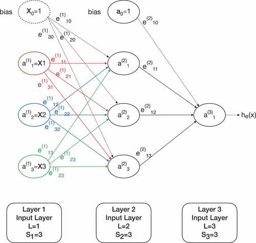
The basic representation of a neural network model is given in Figure 2, having three layers; input layer, hidden layer, and output layer. In Figure 2, “L” represents the layer number, “S” represents the number of units in the layer, “a” represents activations of units, and “θ” is associated with the weights assigned in the network.

Figure 2. Representation of a neural network model.

The learning process involves starting with initial values of the weights ${\theta }_{ij}^{\left(L\right)}$ which is modified at the end of each iteration, which goes through the following four major steps (Shaik et al. 2020).

• Forward-propagation:

The activation of unit “j” in layer “L” ($a_j^{\left(L\right)}$) is calculated by running the network forward with input data to get the network output. The input data are the values of the features $\hspace{0.17em}{X}_i$.

The activation unit is calculated using the sigmoid activation function $\sigma$ (z), as in equation (1)(1) $a_j^{\left(L\right)}=\sigma \left({\theta }^T.\hspace{0.17em}X\hspace{0.17em}\right)=\sigma \left(z\right)=\hspace{0.17em}\frac{1}{1+\hspace{0.17em}{e}^{-z}}$(1)

(1) $a_j^{\left(L\right)}=\sigma \left({\theta }^T.\hspace{0.17em}X\hspace{0.17em}\right)=\sigma \left(z\right)=\hspace{0.17em}\frac{1}{1+\hspace{0.17em}{e}^{-z}}$(1)

• Error calculation:

For each iteration, given a set of training data points (actual outputs) ($y_j$) and the corresponding nodes from the output layer ($a_j^{\left(3\right)}$), we can write the error (E) as in equation (2)(2) $\mathrm{M}\mathrm{i}\mathrm{s}\mathrm{s}\mathrm{i}\mathrm{n}\mathrm{g}\mathrm{o}\mathrm{p}\mathrm{e}\mathrm{n}\mathrm{b}\mathrm{r}\mathrm{a}\mathrm{c}\mathrm{e}\mathrm{f}\mathrm{o}\mathrm{r}\mathrm{s}\mathrm{u}\mathrm{p}\mathrm{e}\mathrm{r}\mathrm{s}\mathrm{c}\mathrm{r}\mathrm{i}\mathrm{p}\mathrm{t}E=\frac{1}{2}\sum _{\hspace{0.17em}}^{\hspace{0.17em}}{\left({a_j}^{\left(3\right)}-y_j\right)}^2$(2) .

(2) $\mathrm{M}\mathrm{i}\mathrm{s}\mathrm{s}\mathrm{i}\mathrm{n}\mathrm{g}\mathrm{o}\mathrm{p}\mathrm{e}\mathrm{n}\mathrm{b}\mathrm{r}\mathrm{a}\mathrm{c}\mathrm{e}\mathrm{f}\mathrm{o}\mathrm{r}\mathrm{s}\mathrm{u}\mathrm{p}\mathrm{e}\mathrm{r}\mathrm{s}\mathrm{c}\mathrm{r}\mathrm{i}\mathrm{p}\mathrm{t}E=\frac{1}{2}\sum _{\hspace{0.17em}}^{\hspace{0.17em}}{\left({a_j}^{\left(3\right)}-y_j\right)}^2$(2)

• Back-Propagation:

Here, $\frac{\mathrm{\partial }E}{\mathrm{\partial }{\theta }_{ij}^{\left(L\right)}}$ the rate of change in the error (E) with respect to each weight in the neural network ${\theta }_{ij}^{\left(L\right)}$ is calculated. This value is used to perform gradient descent with respect to the weights, and then ${\theta }_{ij}^{\left(L\right)}$ is adjusted by propagating it backward through the network.

• Update the weight and biases

Network training is done by generating and choosing values for the weights and biases of the network, and then these weights and biases are modified in each iteration to reduce the error, as represented by equation (3)(3) $\mathrm{\Delta }{\theta }_{ij}^{\left(L\right)}=-\alpha \ast \frac{\mathrm{\partial }E}{\mathrm{\partial }{\theta }_{ij}^{\left(L\right)}}$(3) and equation (4)(4) ${\theta }_{ij\hspace{0.17em}new}^{\left(L\right)}=\hspace{0.17em}{\theta }_{ij\hspace{0.17em}old}^{\left(L\right)}+\mathrm{\Delta }{\theta }_{ij}^{\left(L\right)}$(4) .

(3) $\mathrm{\Delta }{\theta }_{ij}^{\left(L\right)}=-\alpha \ast \frac{\mathrm{\partial }E}{\mathrm{\partial }{\theta }_{ij}^{\left(L\right)}}$(3)

(4) ${\theta }_{ij\hspace{0.17em}new}^{\left(L\right)}=\hspace{0.17em}{\theta }_{ij\hspace{0.17em}old}^{\left(L\right)}+\mathrm{\Delta }{\theta }_{ij}^{\left(L\right)}$(4)

where $\alpha$ is the learning rate (usually set to 0.1) to avoid overfitting and to have small steps toward the minimum error.

The software used in this research is Visual Gene Developer to build the neural network. This software has an ANN toolbox facilitating architecture generation, training, validation, and prediction. The data can be imported as in Microsoft Excel. Different transfer functions, namely, Gaussian, modified Gaussian, sigmoid, modified sigmoid, and hyperbolic tangent are available. Different values for momentum coefficient and learning rate can be used. Before initiating the training process, all the input data should be normalized between 0 and 1. The predicted productivity rates are then used to modify the progress update, which changes the expected delay to be more realistic according to the actual progress at the site.

4.2. Framework

The framework of the periodically modified construction plan is represented in Figure 3. The model mainly consists of mainly two stages. In the first stage, the neural network model analyzes the actual productivity rate and predicts the future productivity rate in order to obtain the updated schedule of the work. In the second phase, a suitable recovery technique is adopted to recover the delay and restructure the schedule to meet the original baseline plan.

Figure 3. The framework of the periodically modified construction plan.

Initially, the baseline plan of a particular activity is considered. In this study, the activity considered is brickwork. Now, the productivity of a particular group “i” named PP(i) and the crew size of Group “i” will calculate the duration required to complete the activity by the members of Group “i”. Now, the brickwork activity with the planned productivity, planned duration, and planned crew size is executed, and the progress update of the work is noted at a particular time period. The actual productivity calculated from the progress update details of the work forms the actual productivity database.

The actual productivity database is then fed into the neural network model. The input of the model includes the number of blocks prepared per day and the data of the most prominent factors affecting productivity including temperature, humidity, and the skill level of both labor and supervisor (Table 1).

The output of the neural network model is the future estimated productivity rate of Group “i” (PF). The future rate is then compared with the planned productivity value. If the future rate is greater than or at least equal to the planned productivity rate (PF ≥ PP(i)), then there will be no chance of delay in the project. If the future productivity rate is less than the planned productivity rate (PF < PP(i)), there is a chance for the project to get behind the schedule. To estimate the actual progress, the durations of the remaining activities are then recomputed based on the predicted productivity rates, which modifies the project update and the expected finish date to more realistic and representative values of the actual progress at the site.

The updated modified schedule is compared with the actual baseline plan/schedule. This comparison reveals if the project is progressing according to the schedule or if the project is behind the planned schedule. If the updated schedule is similar/ahead of the actual plan of the project, then no modification is required in the baseline plan and the remaining activities are executed according to the baseline plan. On the other hand, if the updated schedule is behind the actual plan, the model proceeds to the second stage and various recovery options are adopted to cope up with the delay and meet the actual schedule. The different options considered include activity crashing, fast tracking, and do nothing. Here, activity crashing was found to be the lowest cost option.

In this model, activity crashing is adopted in which extra labors are supplied to carry out the activity. In order to supply more labors, the required number of extra labors should be known. The difference between the planned productivity rate and the future productivity rate gives the extra productivity required to overcome the delay (P(extra)).

The productivity of the next group (PP(i + 1)) is calculated and analyzed to estimate if it can compensate for the requirement of Group “i”. If not, the productivity of other groups i + 2, i + 3 till i+(n−1) are calculated and analyzed till a suitable group to meet the need of Group “i” is found. As the appropriate group to supply productivity to Group “i” is estimated, the required number of masons with their helpers is transferred to Group “i”.

This procedure can thus help in recovering the delay of the project and can be efficiently utilized to meet the actual baseline plan/schedule of a project.

5. Results

Data related to labor skill level, supervisory skill level, temperature, and humidity were selected as inputs, and mason’s productivity for a given working day (i.e., blocks per day) was selected as the output to develop the neural network model. Each datapoint in the dataset is represented as per mason’s productivity inputs and output for a given day.

The data collected included 1487 data points, and it was divided into training set and testing set randomly. The training set included 1046 data points (70% of the total data), and the testing set included 441 data points (30% of the total data). A portion of the test set including 60 data points (5 masons for 2 weeks) was used to validate the model.

The training set of the prediction model includes 1046 data points of the above-mentioned factors and the corresponding labor productivity of all the 132 masons at the construction site throughout 2 weeks (11 working days; 5 working days in Week 1 and 6 working days in Week 2).

After collecting 1046 data points, all the values were then normalized and randomized before feeding them into the neural network. The parameters normalized are number of blocks per day, temperature, humidity, and the skill level. All factors are scaled to a range of [−1:1] where (−1) and (1) are the highest negative and positive effects, respectively.

The normalization is done within [−1,1] using equation (5):

(5) $\mathrm{E}\mathrm{x}\mathrm{t}\mathrm{r}\mathrm{a}\mathrm{c}\mathrm{l}\mathrm{o}\mathrm{s}\mathrm{e}\mathrm{b}\mathrm{r}\mathrm{a}\mathrm{c}\mathrm{e}\mathrm{o}\mathrm{r}\mathrm{m}\mathrm{i}\mathrm{s}\mathrm{s}\mathrm{i}\mathrm{n}\mathrm{g}\mathrm{o}\mathrm{p}\mathrm{e}\mathrm{n}\mathrm{b}\mathrm{r}\mathrm{a}\mathrm{c}\mathrm{e}{x}^n=2\left\{\left(\frac{x-x_{min}}{x_{max}-x_{min}}\right)-1\right\}$(5)

Table

Where:	x^n	Normalized value
	x	Original value
	$x_{min}$	Minimum value in the data range
	$x_{max}$	Maximum value in the data range

The minimum and maximum values of each factor are as follows:

• Temperature (from the weather history): $x_{min}={10}^{o}C\hspace{0.17em}$ and $x_{max}={55}^{o}C$

• Humidity (from the weather history): $x_{min}=18\mathrm{\%}$ and $x_{max}=100\mathrm{\%}$

• Labor and supervisor skills: The minimum and maximum values were calculated using the Excel sheet of the input data.

After that, the normalized data are randomized to be ready to feed it to the neural network.

5.1. Neural network building, training, and prediction

Visual Gene Developer free software was used to build the neural network. The data set was divided into training set and testing set randomly in proportion to 70:30. The training set was used to develop the model. The optimal neural network model with desired performance is obtained by constantly adjusting the weights to obtain minimum error. After performing multiple runs, an optimal network was obtained with an input layer of 4 nodes, 10 nodes in the primary hidden layer, and 5 nodes in the second hidden layer and 1 node in the output layer. The hyperbolic tangent transfer function was selected for the hidden layers. The momentum coefficient and learning rate were also adjusted to obtain the desired model.

Table

Number of input variables	:	4
Number of output variables	:	1
Number of hidden layers	:	2
Learning rate	:	0.0001
Momentum coefficient	:	0.1
Transfer function	:	Hyperbolic tangent
Target error	:	0.00001

After that, the training set was imported to the software in order to start training the network. After 667,193 training cycles, the network reached the following results:

Table

Sum of errors	=	19.820856
Avg. error per output per dataset	=	0.018949
Regression coefficient ($R^2$)	=	0.8389682

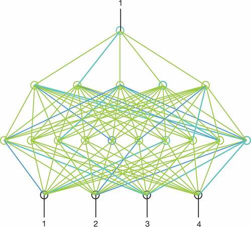
The representation of neural network before and after training is given in Figures (4) and (5), respectively. From Figures (4) and (5), it can be seen that there are four inputs and one output.

Figure 4. Neural network before training.

Figure 5. Neural network after training.

The neural network model obtained after training was tested to verify the performance of the model. The test set without output variable was used to verify the actual and predicted results. The difference in actual value and predicted value of the output as obtained from the software was calculated in percentage and it was found to be 7.11%. Hence, a multilayer feedforward backpropagation was designed and tested. Furthermore, to validate the performance of the neural network model in real a construction project, a sample of the test set related to five masons for 2 weeks was utilized as seen in the next section.

5.2. Validation of the model

To validate the model, one group of labors was selected from a total of 17 groups (Table 2). Group 2 consists of five masons with their helpers, and working in one villa of two floors was selected. The groundfloor block work quantity is 10,000 blocks, and the first-floor block work quantity is 9000 blocks. According to the baseline plan, groundfloor block work activity is planned to finish within the 3 weeks (16 working days) as shown in Table 3.

Table 3. Baseline plan for Week 1 to Week 3.

	Week 1	Week 2	Week 3	Total
Days	3 September 2017 To 7 September 2017	9 September 2017 to 14 September 2017	16 September 2017 to 20 September 2017	16
Planned number of blocks/man-day*	125	125	125	125
Number of days	5	6	5	16
Number of masons	5	5	5	15
Planned blocks	3125	3750	3125	10,000

*The number of blocks/man-day is defined as the daily productivity rate of one group consisting of one mason and one helper

The data from the training set (Week 1 and Week 2) was fed into the machine learning model to compare the actual and planned values as in Table 4. However, instead of planned productivity of 125 blocks/day for each mason, the average productivity was 118.8 blocks/day and 117 blocks/day in the 1^st and 2^nd weeks, respectively. With the neural network model, the actual productivity values obtained for Week 1 and Week 2 are used to update the schedule for Week 3. According to the initial plan, the productivity was expected to be 125 blocks/day. However, the actual value on the field was different. Hence, machine learning the actual productivity will automatically update the construction schedule and prescribe suitable recovery strategies to be adopted to meet the required output.

Table 4. Actual and planned data for Week 1 and Week 2.

Productivity	Activity	Week 1	Week 2	Total
Actual	Number of blocks produced	2970	3510	6480
	Number of blocks /man-day	118.80	117.00
Planned	Number of blocks produced	3125	3750	6875
	Number of blocks /man-day	125.00	125.00

Table 3 implies the total quantity of blocks to be produced by the end of Week 3 is 10,000, and Table 4 shows the actual output from the Week 1 and Week 2 is 6480. Thus, the remaining number of blocks to be manufactured in Week 3 to meet up the planned schedule is calculated and tabulated in Table 5.

Table 5. Data for week 3.

Remaining Quantity	Total planned quantity – Actual quantity of Week 1 and Week 2 = 10,000–6480	3520 blocks
Predicted number of blocks	From the machine learning model	2873blocks
Activity Lag	Remaining quantity – predicted number of blocks = 3520–2873	647 blocks

Thus, the project is behind schedule by 647 blocks that need to be done in Week 3. This shortage is to be compensated by supplying more resources.

Table 6 shows the new proposed analysis of the progress update at the end of Week 2 (on 14 September 2017), which is to modify the expected delay based on the predicted productivity, not the originally planned productivity, which was not achieved by the group.

Table 6. Conventional progress update vs. Modified update based on the machine learning model.

Conventional Progress update				Modified (Machine learned) Progress Update
Description	Symbol	Unit	Value	Description	Symbol	Unit	Value
Elapsed Duration	$D_{EL}$	Days	11	Elapsed Duration	$D_{EL}$	Days	11
Planned total duration	$D_P$	Days	16	Planned total duration	$D_P$	Days	16
Remaining Quantity	$Q_R$	Blocks	3520	Predicted Quantity	$Q_R$	Blocks	2873
Number of masons	MAS	Masons	5	Number of masons	MAS	Masons	5
Planned Daily Crew productivity	$C{P}_{Plan}$ (According to the baseline plan)	Blocks/day	625	Predicted productivity based on machine learning model	(QR/(DP-DEL)	Blocks /day	574.6
Planned mason prod.	$P_P$	Blocks/ mas/day	125	Modified mason prod.	$P_{MOD}$(CPEXP/MAS)	Blocks/ mas/day	114.92
Remaining Duration (conventional)	$D_{RC}$	Days	5.63	Remaining Duration (Modified)	$D_{RM}$	Days	6.13
Conventional Total Duration	$D_{TC}$ (DEL + DRC)	Days	16.63	Modified total duration	$D_{TM}$ (DEL + DRM)	Days	17.13
Conventional delay = remaining duration – week3	$DE{L}_C$($D_{EL}+\hspace{0.17em}\frac{Q_R\hspace{0.17em}}{P_P\ast MAS}-\hspace{0.17em}{D}_P$)	Days	0.63	Modified delay = remaining duration – week3	$DE{L}_M$(DTM-DP)	Days	1.13
Conventional Rounded Delay	$DE{L}_{CR}$	Days	1	Modified Rounded Delay	$DE{L}_{MR}$($D_{EL}+\hspace{0.17em}\frac{Q_R\hspace{0.17em}}{C{P}_{Exp}}-\hspace{0.17em}{D}_P)$	Days	2
Needed Manpower in week 3 to finish on the planned date(Based on $P_p)$	$MA{S}_{NC}$($\frac{Q_R}{P_P\ast \left(D_P-D_{EL}\right)})$	Masons	6	Needed Manpower in week 3 to finish on the planned date (Based on $P_{MOD})$	$MA{S}_{NM}$($\frac{Q_R}{P_{MOD}\ast \left(D_P-D_{EL}\right)})$	Masons	7

The machine learning model predicts the remaining duration based on the actual productivity rates, not the initially planned ones that cannot be achieved, and hence, the model is realistic and practically applicable. According to the conventional progress update one extra mason and according to modified progress update, two extra masons are required to complete the activity on time.

From Table 6, it is concluded that two extra masons with their helpers are needed to provide 647 blocks in week 3 for Group 2. According to the framework which is explained in Figure 3, once the extra productivity [P(extra)] required by Group “i” (here Group 2) is analyzed, the model will check the productivity of other groups one by one [PP(i+(n−1))]. The group which can supply enough resources will be selected to deal with the delay. Group 1 consists of 13 masons (Table 2). Two masons with their helpers were moved from Group 1 to Group 2, both having a total predicted productivity of 1023 (Activity-crashing; more resources are added). Now, the Group 2 consists of seven masons with their helpers. The actual number of blocks observed was 3970 for seven masons. The predicted value was obtained by multiplying the number of days (5 days) with the predicted productivity based on machine learning (574.6 blocks/day) and adding this value to the productivity of the two extra labors (1023 blocks). The predicted and actual values were very close, and the error was too low. This result validates the model.

With the seven masons, the progress of Week 3 was as follows:

Table

Number of blocks (Actual)	=	3970
Number of blocks (Predicted)	=	(574.6*5) + 1023
	=	3896
Error %	=	$\frac{\left(3970-3896\right)}{3970}\ast 100$
	=	1.86%
Accuracy %	=	100% – Error %
	=	98.14%

Thus the model is 98.14% accurate.

• In this study, the calculation of labor skills and supervisory skills is dependent on the number of blocks prepared. This may cause autocorrelation or multicollinearity between the variables in certain situations. An additional similar analysis with independent variables (Temperature and Humidity) was performed, resulting in a model with 92.01% accuracy in contrast to 98.14% in the above model.

6. Discussion

In the present study, a periodically modified project planning approach based on neural network is adopted. The major factors affecting labor productivity were discussed and the most prominent factors such as skill level and environmental factors were used in the case study. The recovery option selected in the approach was activity crashing, in which excess resources are pumped in, to overcome the delay. The algorithm developed was validated, and it was found to be 98.14% accurate. Previous studies on similar approach for recovering the delay also generated promising results (Agyei 2015; Abdul-Rahman et al. 2006).

Apart from the above-mentioned merits, there are certain limitations for the implementation of the proposed prediction approach, which can be addressed in future research. Initially, in this study, the ideal case is considered where the labors are assumed to be present every day for the work. Labors can be absent on one or other day due to various reasons (Durdyev, Omarov, and Ismail 2017). Thus, the effect of labor absence should be considered in the future study.

The factors considered for the development of the model were only labor skill, supervisory skill, temperature, and humidity, due to unavailability of enough data. However, there are many other variables to be considered in a decision-making model (Perera, Sutrisna, and Yiu 2016). Hence, the effect of other factors affecting productivity can be a point of future research. Moreover, in the present study, the recovery option adopted is pumping of additional labor to increase the productivity of the group. However, this assumption is not always valid, especially in the activities with workspace limitations (li, Love, and Drew 2000). Depending on the activity, the number of labors will have an impact on productivity. The relationship between the productivity and the crew size need not always be linear. Hence, for future research, the profile of the relationship between the productivity and the crew size should be subject to the type of activity. Moreover, the workspace limitations should be considered as one of the prominent factors while selecting a recovery action in addition to the cost comparison for each type of recovery actions. Thus, the model works well in ideal case where the labors are not absent in any working day and when the productivity is proportional to the crew size. It is not necessary that the other cases generate the same highly accurate solutions.

The accuracy of the model was lesser when only environmental factors were considered. This implies that the performance of the model is associated with the type of input variables selected for the study. In the future, consideration of additional input variables which can closely represent the physical and physiological data of the labors, years of experience, etc., may increase the applicability of the model. The advancement in data collection techniques, such as collecting data via sensors and cameras, is increasing the availability of data compared to previous days (Yu et al. 2021). The activity focused in this study is the block work, and the data associated with this activity are utilized to develop the model. The scope of this novel approach can be improved by considering additional construction activities like plastering, painting, etc., in future studies.

This study implies the possibility of cost and time management in construction projects with periodically modified construction plans. The study ensures that the huge amount of money spent by construction firms on recovery plans can be substituted with simple cheap solutions through periodic monitoring and self-recovering schedules. This study can be considered as an initial step for the development of similar models in the future by including more factors and different scenarios.

7. Conclusion

Delays are an indispensable feature of the construction industry. The periodically modified construction plan using FFNN with backpropagation learning algorithm developed in this research can be used to develop self-recovering schedules. The features of the machine learning approach developed include predicting future productivity rates and automated recovery actions’ calculations, followed by a cost optimization algorithm to choose a suitable recovery action. In the present study, the approach is validated with a case study, and it is found to be more than 98% accurate.

Moreover, the modified progress update provides a realistic expectation of the delay at site because it was based on actual data and not based on planned data. Here, the schedule is continuously updated with the actual progress of the activity at the site. When construction plans are regularly updated with real data, the delay can be easily captured at an early stage. This would help the decision-makers to adopt suitable and cheap recovery actions in the initial phase of the activity delay. Moreover, the application of neural networks and machine learning techniques can improve the scope, accuracy, and applicability of this scheduling approach.

This research project is expected to be an eye-opener for the continuously modified construction plans. The results obtained in this study imply that developing the model further with the addition of more factors, which causes delay in projects, can lead to better cost and time management compared to conventional project recovery methods. The modeling approach developed in this research should be particularly useful for projects where significant cost savings and high standards in terms of both quality and time management are likely to be the most important.

Disclosure statement

No potential conflict of interest was reported by the author(s).

Additional information

Funding

The authors are grateful to the UAE University for the facilities provided for research. This research was financially supported by the Research Affairs Office at UAE University under grant number 12R099

Notes on contributors

Hamad AlJassmi

Hamad AIJassmi is the Director of EmiratesCenter for Mobility Research (ECMR) at UAEUniversity. He is an Associate Professor of Civil Engineering at UAE University, and a ResearchFellow of University of New South Wales, Sydney.Apart from academia, Dr. Al Jassmi acted as Project Director, Project Manager or Project Leadat numerous consultancy projects related to trafficsafety, mobility policy making and planning. He obtained his PhD in Construction Engineering Management from the School of Civil Environmental Engineeringat UNSW in Australia. In his thesis, he developed mathematical methodsthat serve for analysing the complex generative mechanisms of defectsin construction. His research interests include expert systems and machinelearning for the buildings and infrastructure sector. He published more than50 peer-reviewed articles, several which appeared in top ranked international journals.

Yusef Abduljalil

Yusef Abduljalil is a Senior Planning Engineer with a knack for ensuring that projects are planned and executed efficiently. Adept at employing diverse building methods to achieve project goals. Yousef’s point of strength is his knowledge and experience in delay analysis, as well as implementing the latest methods in project planning and control.

Babitha Philip

Babitha Philip is a research assistant at the Emirates Center for Mobility Center (ECMR), UAE University. She is a PhD candidate at the Civil and Environmental Engineering Department, UAE University. Babitha completed her master's in Construction Engineering and Management and bachelor's in Civil Engineering from India. Babitha’s research works focus on application of Artificial Intelligence techniques in civil engineering field.

References

- Abdul-Rahman, H., M. A. Berawi, A. R. Berawi, O. Mohamed, M. Othman, and I. A. Yahya. 2006. “Delay Mitigation in the Malaysian Construction Industry.” Journal of Construction Engineering and Management 132 (2): 125–133. doi:10.1061/(ASCE)0733-9364(2006)132:2(125).
- Agyei, W. 2015. “And CPM Techniques With Linear Programming : Case Study.” International Journal of Scientific & Technology Research.
- Al-Zwainy, F. M. S., H. A. Rasheed, and H. F. Ibraheem. 2012. “Development of the Construction Productivity Estimation Model Using Artificial Neural Network for Finishing Works for Floors with Marble.” ARPN Journal of Engineering and Applied Sciences.
- Babu, A. J. G., and N. Suresh. 1996. “Project Management with Time, Cost, and Quality Considerations.” European Journal of Operational Research 88 (2): 320–327. doi:10.1016/0377-2217(94)00202-9.
- Ballesteros-Pérez, P., K. M. Elamrousy, and M. C. González-Cruz. 2019. “Non-linear time-cost trade-off Models of Activity Crashing: Application to Construction Scheduling and Project Compression with fast-tracking.” Automation in Construction 97 (November 2018): 229–240. doi:10.1016/j.autcon.2018.11.001.
- Durdyev, S., M. Omarov, and S. Ismail. 2017. “Causes of Delay in Residential Construction Projects in Cambodia.” Cogent Engineering 4 (1): 1291117. doi:10.1080/23311916.2017.1291117.
- Feylizadeh, M. R., A. Mahmoudi, M. Bagherpour, and D. F. Li. 2018. “Project Crashing Using A Fuzzy multi-objective Model considering Time, Cost, Quality and Risk under Fast Tracking Technique: A Case Study.” Journal of Intelligent and Fuzzy Systems 35 (3): 3615–3631. doi:10.3233/JIFS-18171.
- Gerek, I. H., E. Erdis, G. Mistikoglu, and M. Usmen. 2015. “Modelling Masonry Crew Productivity Using Two Artificial Neural Network Techniques.” Journal of Civil Engineering and Management. doi:10.3846/13923730.2013.802741.
- Guida, P. L., and G. Sacco. 2019. “A Method for Project Schedule Delay Analysis.” Computers and Industrial Engineering 128 (December 2018): 346–357. doi:10.1016/j.cie.2018.12.046.
- Hady, H. N., L. A. Al-Kindi, and M. A. Mahmoud (2020). “Construction Project Planning Using Integration of Crashing and Concurrency Techniques.” IOP Conference Series: Materials Science and Engineering. Istanbul, Turkey, 737(1). https://iopscience.iop.org/article/10.1088/1757-899X/737/1/012037/meta
- Harun, T., P. Gul, D. Atilla, and A. Firat Dogu. 2020. “Project Crashing with Crash Duration Consumption Rate: An Illustrative Example.” 56–64. doi:10.3311/ccc2020-046.
- Heravi, G., and E. Eslamdoost. 2015. “Applying Artificial Neural Networks for Measuring and Predicting Construction-Labor Productivity.” Journal of Construction Engineering and Management 141 (10). doi:10.1061/(asce)co.1943-7862.0001006.
- Jang, H., K. Kim, J. Kim, and J. Kim. 2011. “Labour Productivity Model for Reinforced Concrete Construction Projects.” Construction Innovation 11 (1): 92–113. doi:10.1108/14714171111104655.
- Leu, S. S., A. T. Chen, and C. H. Yang. 2001. “A GA-based Fuzzy Optimal Model for Construction time-cost trade-off.” International Journal of Project Management 19 (1): 47–58. doi:10.1016/S0263-7863(99)00035-6.
- li, H., P. E. D. Love, and D. S. Drew. 2000. “Effects of Overtime Work and Additional Resources on Project Cost and quality.” Engineering, Construction and Architectural Management 7 (3): 211–220. doi:10.1108/eb021146.
- Lock, D. 2017. “The Essentials of Project Management, Fourth Edition.” The Essentials of Project Management. Fourth Edition. doi:10.4324/9781315239941.
- Martens, A., and M. Vanhoucke. 2019. “The Impact of Applying Effort to Reduce Activity Variability on the Project Time and Cost Performance.” European Journal of Operational Research 277 (2): 442–453. doi:10.1016/j.ejor.2019.03.020.
- Perera, N. A., M. Sutrisna, and T. W. Yiu. 2016. “Decision-Making Model for Selecting the Optimum Method of Delay Analysis in Construction Projects.” Journal of Management in Engineering 32 (5). doi:10.1061/(asce)me.1943-5479.0000441.
- Rivas, R. A., J. D. Borcherding, V. González, and L. F. Alarcón. 2011. “Analysis of Factors Influencing Productivity Using Craftsmen Questionnaires: Case Study in a Chilean Construction Company.” Journal of Construction Engineering and Management 137 (4): 312–320. doi:10.1061/(asce)co.1943-7862.0000274.
- Shaik, N. B., S. R. Pedapati, S. A. Ammar Taqvi, A. R. Othman, and F. A. Abd Dzubir. 2020. “A feed-forward Back Propagation Neural Network Approach to Predict the Life Condition of Crude Oil Pipeline.” Processes 8 (6): 661. doi:10.3390/PR8060661.
- Sindhu, J., K. Choi, S. Lavy, Z. K. Rybkowski, B. F. Bigelow, and W. Li. 2018. “Effects of Front-End Planning under Fast-Tracked Project Delivery Systems for Industrial Projects.” International Journal of Construction Education and Research 14 (3): 163–178. doi:10.1080/15578771.2017.1280100.
- Umit Dikmen, S., and M. Sonmez. 2011. “An Artificial Neural Networks Model for the Estimation of Formwork Labour.” Journal of Civil Engineering and Management. doi:10.3846/13923730.2011.594154.
- Yu, Y., W. Umer, X. Yang, and M. F. Antwi-Afari. 2021. “Posture-related Data Collection Methods for Construction Workers: A Review.” Automation in Construction 124 (November 2019): 103538. doi:10.1016/j.autcon.2020.103538.