Investigation of the time-dependent dynamics between government revenue and expenditure in China: a wavelet approach

Abstract

Unlike previous studies on causal relationships between government revenue and expenditures in China, this study takes into consideration structural breaks in the data by performing wavelet decomposition prior to testing for Granger causality between the fiscal components. The use of wavelet decomposition is motivated by economic theories, which suggest allowing for different budgetary considerations at different time horizons, as well as by the existence of special properties in the data in the form of unit roots and structural breaks. The results from the Granger causality test when using the wavelet-decomposed quarterly data over the period 1980–2015 indicate that government revenue Granger-causes government expenditure (tax-and-spend hypothesis) in the wavelet scales of two to four quarters. The results also show that bidirectional causality (fiscal synchronisation) exists in the wavelet scale of eight to sixteen quarters. Understanding the causal relationships between revenue and expenditure at different time scales is important for formulating relevant policy measures in order to maintain fiscal sustainability in China.

Keywords:

• Government revenue
• government expenditure
• fiscal sustainability
• Granger causality
• wavelet analysis

1. Introduction

Interest in the nexus between government revenue and expenditure is not new. Considerable research has been performed in this area, generating hot debates on the use of deficit financing and its effects on sustainability. In recent years, in conjunction with the financial crisis during 2008–2009, the merits of fiscal policy have been even more under the spotlight. The relationship between government revenue and expenditure is connected to budgetary policies, which are of importance for formulating a sustainable fiscal policy (Brady and Magazzino 2019). The current study has interest in the relationship between government revenue and expenditure in China for two reasons. First, China is the second largest economy in the world, so the relationship between the revenue and expenditure of its public sector has implications for the global economy, as is reflected by the recent media coverage regarding the increasing government budget deficit of China during recent years.¹ Second, as noted by Li (2001), the institutional, structural and organisational characteristics of China are distinctly different from those of other developed economies of the G7 countries. Studies on the relationship between government revenue and expenditure in China are relatively few compared to such studies for developed economies. There are some recent studies in this area that include China in a panel setting; however, the study at hand focuses only on the case of China with the aim of delving into the country-specific causality patterns that can be different from other economies.

Studies on the relationship between government revenue and expenditure are centred on exploring their causal relationships, and these relationships have important implications for the budget deficit and sustainability. The causal relationships are categorised by four hypotheses: (1) tax-spend, (2) spend-tax, (3) fiscal synchronisation and (4) institutional separation. The first hypothesis, the tax-spend hypothesis, was advocated by Friedman (1978) who asserted that raising taxes will lead to more spending by the government, so a reduction of the budget deficit is unlikely. Under this proposition, budget deficits can be decreased only with a reduction in government expenditure. The direction of causality runs from revenue to expenditure in this case. The second hypothesis argued by the spend-and-tax school supports the opposite direction of the causality pattern from the tax-spend school. Peacock and Wiseman (1979) explained that a temporary increase in government expenditures in an economic downturn will lead to a permanent increase in taxes. Their view was shared by Barro (1979) who argued that the ultimate sources of government expenditures are higher future taxes, due to the Ricardian equivalence proposition. The third hypothesis, the fiscal synchronisation hypothesis, advocates that decisions on government revenue and expenditure are made jointly; hence, it implies bidirectional causality (a feedback mechanism) between government revenue and expenditure. Under this situation, the fiscal authorities of the government should raise revenue and decrease expenditure concurrently in case the budget deficit poses a problem for sustainability. The last hypothesis is fiscal neutrality, which is also known as the institutional separation hypothesis. According to this view, decisions on government taxes and expenditures are separately made by different institutions (Baghestani and McNown 1994; Wildavsky 1988), leading to no causality between government revenue and expenditures. Budget deficits and, consequently, government debts would grow under this scenario since decisions on revenues and expenditures are separate. Wolde-Rufael (2008) explained that fiscal neutrality could be due to the disagreement among different parties involved in the budgetary process.

These four different directions of causalities have associations with time horizons, as suggested by the economic theories in this area. In the short run, with rigid wages and prices, fiscal policy can play a role in easing the adjustments to shocks and keeping the production level close to the potential output. Generally, expansionary policy leads to higher budget deficits, and contractionary policy reduces deficits, making such budget deficits or surpluses in the short-run rather casual observations. However, if a government has a deficit, it adds to the government’s net debt. If the government maintains a budget deficit for a prolonged period of time, it poses two relevant problems. First, higher government debt levels make the interest rate rise, which, in turn, makes borrowing even harder to repay the debt. Second, interest rate hikes caused by government borrowing can dampen investment activities, which can hamper long-run economic growth. Thus, a stable debt ratio should be considered in the long run.

To investigate the causality patterns between government revenue and expenditure in China at different time horizons, the current paper employs wavelet decomposition. Wavelet analysis provides a remedy to some of the problems of traditional methods of cointegration and error-correction models (ECMs) that arise due to particular properties of the data, namely, mixed results on nonstationarity and structural breaks. Using wavelet analysis has some advantages over the traditional methods of ECMs and cointegration for studying short- and long-run relationships. First, losing relevant variable information from taking first differences to make a nonstationary series stationary can be avoided by using wavelets. Second, instead of using a blunt short- and long-run dichotomy on variable relationships, time scales that are associated with changes that occur after one, two or four periods and so on can be specified (more specific explanations on time scales in the wavelet domain follow in Section 3). This decomposition of time scales is arguably more desirable than ambiguously categorising time scales into short- and infinitely-long long-term relationships. This advantage of wavelet analysis of decomposing a series into different time scales has made it increasingly popular recently (Ramsey and Lampart 1998; Percival and Walden 2000; Almasri and Shukur 2003; Hacker, Karlsson, and Månsson 2012, 2014, among others).

The results from this study, using the wavelet decomposition technique, indicate that government revenue Granger-causes government expenditure at the wavelet scale of two to four quarters, while the bidirectional Granger causality is present at the wavelet scale of eight to sixteen quarters. Bidirectional causality between these variables was documented in previous studies on China (Li 2001; Chang and Ho 2002; Ho and Huang 2009). However, the current paper discloses some time-varying relationships of these economic variables at different time scales and clarifies the cycles when bidirectional causality is detected. Therefore, this study makes a modest contribution to the empirical literature by unveiling the relationship between government revenue and expenditure using Chinese data at different time horizons.

The rest of the paper is organised as follows. Section 2 provides an overview of the literature on the links between government revenue and expenditure. Section 3 presents the methodologies used in the paper, followed by the data description and preliminaries in Section 4. Empirical results are presented in Section 5. In Section 6, some concluding remarks are offered.

2. Literature review

Numerous studies have examined the causality patterns of government revenue and expenditure for different countries. These studies have used different econometric methods, different measures on government revenue and expenditure, and different sample periods. Not surprisingly, varying or conflicting results between these studies are apparent in some cases.

Early studies on the relationship between government revenue and expenditure focussed on developed economies. For example, Owoye (1995) studied the causal relationship between government revenue and expenditure of G7 countries using cointegration and ECMs. Using annual data from 1960 to 1990, Owoye found bidirectional causality patterns in most G7 countries with the exceptions of Japan and Italy, where the tax-spend hypothesis was supported. More recently, Afonso and Rault (2009) investigated causality between government spending and revenue in the EU for the period 1960–2006 using a newly developed method for econometric technical bootstrap panel analysis. Two different groups of countries have shown different causality patterns: while spend-tax causality is found for Italy, France, Spain, Greece and Portugal, tax-and-spend evidence is documented for Germany, Belgium, Austria, Finland and the UK, as well as for several EU new member states. In a country-specific study, Athanasenas, Katrakilidis, and Trachanas (2014) re-evaluated the long-run relationship between government revenues and expenditures in Greece over the period 1999–2010 using asymmetric ARDL cointegration methodology. They found supporting evidence of asymmetric interactions between the government revenue and expenditure in both long- and short-run time horizons. Dalena and Magazzino (2012) studied the long-run relationship between government expenditure in Italy over 100 years (1982–1993) and documented that different hypotheses hold in different sub-periods, which reflects the prevailing paradigms of public finance in different periods.

The empirical results on the relationship between government revenue and expenditure are very mixed in African countries as well. Using a VAR approach, Nyamongo, Sichei, and Schoeman (2013) documented that government revenue and expenditures in South Africa are cointegrated and also reported a bidirectional Granger causality. Wolde-Rufael (2008) examined 13 African countries using the Toda and Yamamoto (1995) causality test, where all four directions of causation described earlier were found. Bidirectional causality was found between expenditure and revenue for Mauritius, Swaziland and Zimbabwe, while no causality was detected in any direction for Botswana, Burundi and Rwanda. Unidirectional causality from revenue to expenditure applied for Ethiopia, Ghana, Kenya, Nigeria, Mali and Zambia, whereas unidirectional causality running from expenditure to revenue was only present for Burkina Faso. Magazzino (2013) assessed the relationship of the countries in the Economic Community of West African States (ECOWAS) and reported mixed results from Granger causality analysis of the government revenue and expenditure for West African Economic and Monetary Union (WAEMU) countries, while showing that for four countries (Gambia, Liberia, Nigeria and Sierra Leone) out of the six West African Monetary Zone (WAMZ) countries, the tax-spend hypothesis held.

Studies on the relationship between government revenue and expenditure were also done for Asian economies. Park (1998) studied the possibility of Granger causality between government revenue and expenditures in Korea using annual data from 1964–1992, reporting evidence for the tax-spend hypothesis. In the case of Malaysia, Hong (2009) employed a Johansen cointegration test and an ECM for causality using annual data between 1970 and 2007. He documented a long-run relationship between government revenue and expenditure and presented evidence for the spend-and-tax hypothesis in Malaysia. A group of Asian countries were studied regarding the government revenue-expenditure relationship in a panel setting. Out of the nine countries studied by Narayan (2005), only three countries showed a long-run cointegration relationship, and the Granger causality results were very mixed for the countries included over the period from 1960–2000. More recently, Magazzino (2014) revisited the relationship between revenue and expenditure in the ASEAN countries using annual data from 1980–2012. Mixed results were also documented, with a predominance of support for the tax-spend hypothesis.

Within the vast literature on this topic of government revenue and expenditure nexus, empirical studies on China and one study that used wavelet analysis are more relevant to the current study than others. Li (2001) performed an in-depth study, testing for unit roots and cointegration and estimating VAR as well as VECM models. Using annual data over the period 1950–1997, it was documented that bidirectional causality exists between government expenditure and revenue in China. Chang and Ho (2002) tested this relationship for China over the period 1977–1999 and found bidirectional causality. In a more recent study, Ho and Huang (2009) tested the same propositions using data on the 31 Chinese provinces covering the period 1999–2005. Based on multivariate panel ECMs, their results differ for the short run and the long run: no significant causality between revenues and expenditures in the short run was found; however, in the long run, the fiscal synchronisation hypothesis was supported for Chinese provinces over the period 1999–2005.

Finally, one more empirical study to be noted here is that by Almasri and Shukur (2003), who employed a wavelet analysis to examine the relationship between government revenue and expenditure in the Finnish economy. Using monthly data over the period 1960–1998, the causality patterns of the two fiscal components were studied in two different subsample periods (1960–January 1990; February 1990–September 1998) as well as for the whole sample period. A strong causality from the expenditure to revenue in the second subsample period was documented at the finest and intermediate scales (although inconclusive results were reported for the larger scales), which is in line with the political system change in Finland around that time period regarding the country’s future plans of being a member of the European monetary union. This study is noteworthy because it examined the causal relationship between government revenue and expenditure at different time horizons using wavelet analysis, which not only helped separate the time-scale structured relationship but also turned the nonstationary series into stationary ones.

3. Methodologies

3.1. Causal analysis for bivariate vector autoregression model

For a bivariate VAR model (i.e. a two-equation model), $x_t$ and $y_t$ are defined by the following: (3.1) $$\left[\begin{array}{c}{x}_t\\ y_t\end{array}\right]=\left[\begin{array}{c}{Z}_{10}\\ Z_{20}\end{array}\right]+\left[\begin{array}{cc}{Z}_{11}{}^{\left(L\right)}& Z_{12}{}^{\left(L\right)}\\ Z_{21}{}^{\left(L\right)}& Z_{22}{}^{\left(L\right)}\end{array}\right]\left[\begin{array}{c}{x}_{t-1}\\ y_{t-1}\end{array}\right]+\left[\begin{array}{c}{e}_{\mathit{xt}}\\ e_{\mathit{yt}}\end{array}\right],$$(3.1) where $Z_{i0}$ denotes the parameters representing the intercept terms and $Z_{\mathit{ij}}{}^{(L)}$ is the polynomial in the lag operator L. Moreover, $x_t$ and $y_t$ are stationary, and $e_{\mathit{xt}}$ and $e_{\mathit{yt}}$ are uncorrelated white-noise disturbances. The variable $y_t$ does not Granger-cause $x_t$ if ${Z_{12}}^{\left(i\right)}=0$ , for $i=1,\mathrm{ }2,\dots p$. That is, Granger causality is directly tested using a standard F-test of the restriction: (3.2) $$Z_{12}{}^{\left(1\right)}=Z_{12}{}^{\left(2\right)}=Z_{12}{}^{\left(3\right)}\dots =Z_{12}{}^{\left(p\right)}=0$$(3.2)

For ease of illustration, we can focus on the bivariate AR(1) process. The hypotheses regarding the directions of causality between x and y that can be tested in such a process are as follows:

1. y causes x but x does not cause y, $H_1$, $$H_1=\left[\begin{array}{cc}{Z}_{11}& Z_{12}\ne 0\\ 0& Z_{22}\end{array}\right]$$

2. x causes y but y does not cause x, $H_2$, $$H_2=\left[\begin{array}{cc}{Z}_{11}& 0\\ Z_{21}\ne 0& Z_{22}\end{array}\right]$$

3. Feedback, $H_3$ $$H_3=\left[\begin{array}{cc}{Z}_{11}& Z_{12}\ne 0\\ Z_{21}\ne 0& Z_{22}\end{array}\right]$$

4. Independent, $H_4$ $$H_4=\left[\begin{array}{cc}{Z}_{11}& 0\\ 0& Z_{22}\end{array}\right]$$

3.2. Toda-Yamamoto causality test

As noted in the subsection above, testing Granger causality requires that all the variables in the VAR system are stationary. When the variables are not stationary and not cointegrated, testing Granger causality in the traditional way can lead to spurious causality. Toda and Yamamoto (1995) proposed a procedure that does not require the cointegration of the nonstationary variables. The procedure involves first testing for integration with structural breaks considered. After the maximum order of integration is determined, the VAR model is set up in levels, and the lag length, p, should be determined. If the residuals are not serially correlated, the maximum order of integration is added to the number of lags. This makes the procedure an augmented VAR model, which guarantees the asymptotic distribution of the Wald statistic. To thoroughly explore the data prior to decomposition, Granger-causality testing is performed on the raw data, and for that testing the Toda-Yamamoto causality procedure is implemented due to the finding of possible nonstationarity in the variables.

3.3. Wavelet decomposition

As a remedial solution to the limitations of the robustness properties of traditional methods and to analyse time-scale relations for non-cointegrated variables, wavelet analysis is used in this paper. Wavelets means, as the name suggests, small waves compared to the big waves, such as the sine function. Such small waves can be either ‘stretched’ or ‘squeezed’ to approximate variables locally in time or space with the help of their ability to mimic the series under investigation (Crowley 2007). Wavelet analysis allows us to conduct a very robust analysis by decomposing data at various time scales, while it enables controlling for nonstationary trends, autocorrelation, heteroscedasticity and structural breaks (Ramsey and Lampart 1998; Schleicher 2002; Benhmad 2012; Hacker, Karlsson, and Månsson 2014, among others). One of the non-technical descriptions of the wavelet decomposition of a series of observations is comparing it to the activity of a camera lens. Zooming out the lens brings a broad landscape and zooming in allows the observation of details that were not observable in the landscape scenery. In mathematical terms, ‘wavelets are local orthonormal bases consisting of small waves that dissect a function into layers of different scale’ (Schleicher 2002, 1).

In this paper, each of the time series is decomposed through the methodology referred to as maximum overlap discrete wavelet transform (MODWT), which uses moving averages of the original data and moving averages of moving averages (Hacker, Karlsson, and Månsson 2014). In each step, if each value in the series on which the averages are being taken is used only once in computing the averages and (assuming the use of the Haar function) if the averages are simply between pairs of contiguous values, then, with some standard normalisation, this results in a (non-overlapping) discrete wavelet decomposition (DWT). Under DWT, the wavelet transformation is orthogonal, providing just enough information from the averages at one scale along with differences from averages at that scale² and lower scales to reconstruct the original series. The weakness of the DWT, however, is that it suffers from sensitivity to the point at which one starts the averaging, and it is very limited to the observation sizes that correspond only to the didactic series (N = 2ⁿ for some integer n). Moreover, the distinct values from the averages using DWT become fewer as the scale increases because a value from the original series can be used only once for the average calculations at a particular scale. The data used in the current paper are quarterly data over a period of 35 years, and this limited number of observations in our dataset for wavelet analysis is severe. Therefore, as an alternative, the MODWT is instead used in this paper.³

A quick way of performing wavelet decomposition is through a multiresolution analysis (MRA), a methodology that was introduced by Mallat (1989). Understanding how the calculations for the smooth and detail series for the MRA of the MODWT are performed with the Haar function can be illustrated from the following example. Let y be a vector of actual time series observations. By convention in the wavelet literature, s_j and d_j, denote smooth and detail series at level j, respectively. The following two formulae describe how the smooth and detail series are calculated at scale levels of 1 and higher: (3.3) $$s_{j,t}=\frac{s_{j-1,t-2^{j-1}}+2s_{j-1,t}+s_{j-1,t+2^{j-1}}}{4},$$(3.3) (3.4) $$d_{j,t}=\frac{-s_{j-1,t-2^{j-1}}+2s_{j-1,t}-s_{j-1,t+2^{j-1}}}{4}.$$(3.4)

For illustration, the pattern of how these equations work for three scale levels is demonstrated below. It should be noted that s_0,t = y_t, so that, at scale levels 1, 2 and 3, respectively, we have the following: (3.5) $$s_{1,t}= \left(y_t{}_{-1}+ 2y_t+y_t{}_{+1}\right)/4\text{\hspace{0.5em}and\hspace{0.5em}}{d}_{1,\mathrm{t}}= \left(-y_t{}_{-1}+ 2y_t–y_{\mathrm{t}+1}\right)/4,$$(3.5) (3.6) $$s_{2,t}= \left(s_{1,\mathrm{t}-2}+ 2s_{1,\mathrm{t}}+s_{1,t+2}\right)/4\text{\hspace{0.5em}and\hspace{0.5em}}{d}_{2,\mathrm{t}}= \left(-s_{1,\mathrm{t}-2}+ 2s_{1,t}–s_{1,t+2}\right)/4,$$(3.6) (3.7) $$s_{3,t}= \left(s_{2,t-4}+ 2s_{2,\mathrm{t}}+s_{2,\mathrm{t}+4}\right)/4\text{\hspace{0.5em}and\hspace{0.5em}}{d}_{3,t}= \left(-s_{2,t-4}+ 2s_{2,t}–s_{2,t+4}\right)/4,$$(3.7)

A very nice and desirable feature of this process is that the original series may always be reconstructed by adding the detail series to the smooth series of the largest scale level considered, J, as seen in the equation below: (3.8) $$y=s_J+{\sum }_{j=1}^J{d}_j.$$(3.8)

Conveniently, MRA provides a rather intuitive interpretation of the wavelet decomposition. Simply put, it is a matter of finding (weighted) averages and differences from those averages. The process first starts with values in the series closest to each other (i.e. the lowest scale), then the same process is repeated with the previous average series, which gradually expands how many of the original data are included in each successive average (with increasing the scale). The long-term trend of a variable at the scale level of J is given by $s_J$, which contains the nonstationary components of the original series, if there are any. The original series decomposition at various time scales is given by the detail series $d_1$ to $d_J$ (Hacker, Karlsson, and Månsson 2014).

4. Data and preliminaries

The data used in this paper are the quarterly data of government revenue and expenditure as a share of gross domestic product (GDP) over the period 1980–2015. The data are retrieved from the Thomson Reuters DataStream and are based on the general government revenue (CHXGRE%) and expenditure (CHXGEX%).⁴ Figure 1 shows that the shares of government revenue and expenditure to GDP were very close to each other during the 1980s and the early 1990s. Two aspects are notable here. One is that both ratios have trended downwards until the middle of the 1990s. Since then, they turned to have an upward trend. The other is that the volatilities of the two ratios increased starting around 2007. These two items observed from the time plot of the data lead to the suspicion of structural breaks, which are very important issues to consider in time series analysis.

Figure 1. Government revenue and expenditure as percentage of GDP.

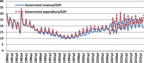
Due to the strong seasonality of the quarterly data, it was deseasonalised using seasonal dummies. Before performing the wavelet analysis, data properties including the unit root and cointegration were examined. The unit roots were tested using five different unit root tests: the augmented Dickey-Fuller (ADF) test; Phillips-Perron (PP) test; Dickey-Fuller test with GLS (DF-GLS) detrending; Elliott, Rothenberg, and Stock (ERS) point optimal test (1996) and the Kwiatkowski, Phillips, Schmidt, and Shin (KPSS) test (Kwiatkowski et al. 1992). In performing all tests, both models with the constant only and with the trend are examined. It should be noted that the null hypothesis of having the unit root applies to all the tests except the KPSS test, which has (trend) stationarity as the null hypothesis. The unit root test results in levels (Table 1) show very mixed results on the unit root with some dominance on the existence of the unit root. It is also notable that the results of the ADF and PP tests are conflicting.⁵ Using first-differenced data (Table 2), however, the null hypothesis of having a unit root is rejected for all the models of the ADF and PP tests. The DF-GLS and ERS tests still show mixed results with first-differenced data, yet to a lower degree compared to using data in levels, while the KPSS test results fail to reject the null hypothesis of stationarity. An exception to the KPSS test results using first-difference data occurs when investigating the data properties for the variable, government expenditure ratio to GDP in log (the model with the constant only), for which stationarity of the first-differenced data is rejected at the 10% level of significance. Critical values of all these unit root tests are included in Table 3. The existence of structural breaks makes the test results of the traditional unit root tests with the unit root as the null hypothesis unreliable because it is well known that such tests suffer from structural breaks in the series being potentially confused as being evidence of nonstationarity, thereby making the unit root test results biased toward unit root (i.e. the test has low power) (Perron 1989) Table 3.

Table 1. Unit root test without structural break at levels.

Variables		ADF	PP	DF-GLS	ERS	KPSS
GR/GDP	Constant	−1.113	−4.809***	−0.482	2.603**	0.345
	With trend	−1.290	−4.819***	−0.3	4.848**	0.329***
GE/GDP	Constant	−0.927	−6.558***	−0.558	1.371	0.353*
	With trend	−1.171	−6.626***	−0.363	.989***	0.320***

Notes: GR/GDP denotes government revenue ratio to GDP in log; GE/GDP denotes government expenditure ratio to GDP in log. Lags are selected based on the Schwarts information criteria. Single (*), double (**) and triple asterisks (***) indicate statistical significance at 10%, 5% and 1% levels, respectively. ADF, PP, DF-GLS, ERS and KPSS are Augmented Dickey-Fuller test, Phillips-Perron test, Dickey-Fuller Test with GLS Detrending, Elliot, Rothenberg, and Stock Point Optimal (ERS) Test and the Kwiatkowski, Phillips, Schmidt, and Shin (KPSS) Test, respectively. ADF, PP and DF-GLS have null hypothesis is that the series has a unit root while KPSS null hypothesis is that the series is stationary. Barlett kernel is used for PP, ERS and KPSS. Critical values are presented in Table 3 below.

Table 2. Unit root test without structural break at 1st difference.

Variables		ADF	PP	DF-GLS	ERS	KPSS
GR/GDP	Constant	−5.500***	−22.608***	−0.248	3.042**	0.224
	With trend	−7.698***	−23.791***	−1.767	8.774	0.076
GE/GDP	Constant	−5.906***	−34.716***	−0.170	3.736*	0.377*
	With trend	−8.171***	−37.993***	−1.318	10.099	0.051

Notes: GR/GDP denotes government revenue ratio to GDP in log; GE/GDP denotes government expenditure ratio to GDP in log. Lags are selected based on the Schwarts information criteria. Single (*), double (**) and triple asterisks (***) indicate statistical significance at 10%, 5% and 1% levels, respectively. ADF, PP, DF-GLS, ERS and KPSS are Augmented Dickey-Fuller test, Phillips-Perron test, Dickey-Fuller Test with GLS Detrending, Elliot, Rothenberg, and Stock Point Optimal (ERS) Test and the Kwiatkowski, Phillips, Schmidt, and Shin (KPSS) Test, respectively. ADF, PP and DF-GLS have null hypothesis is that the series has a unit root while KPSS null hypothesis is that the series is stationary. Barlett kernel is used for PP, ERS and KPSS. Critical values are presented in Table 3 below.

Table 3. Critical values of the unit root tests.

Models	ADF			PP			DF-GLS			ERS			KPSS
	1%	5%	10%	1%	5%	10%	1%	5%	10%	1%	5%	10%	1%	5%	10%
Constant	−3.78	−2.88	−2.58	−3.48	−2.89	−2.58	−2.58	−1.94	−1.62	1.93	3.14	4.24	0.74	0.46	0.35
With trend	−4.03	−3.44	−3.15	−4.02	−3.44	−3.15	−3.53	−2.99	−2.70	4.17	5.65	6.82	0.22	0.15	0.12

Notes: ADF, PP, DF-GLS, ERS and KPSS are Augmented Dickey-Fuller test, Phillips-Perron test, Dickey-Fuller Test with GLS Detrending, Elliot, Rothenberg, and Stock Point Optimal (ERS) Test and the Kwiatkowski, Phillips, Schmidt, and Shin (KPSS) Test, respectively.

Thus, as a next step, the unit root test is performed by considering structural breaks. Numerous studies have suggested different testing methods on the unit root test with structural breaks since the works done by Nelson and Plosser (1982) and, subsequently, Perron (1989) (Glynn, Perera, and Verma (2007) presented a good summary on them). Among these different test methods, the Zivot and Andrews (1992) model for the unit root test with a structural break is used in this paper. This test allows a time series to have one endogenously chosen structural break in the series, which may appear in the intercept, trend, or both. The test was done for both cases (i.e. structural break in trend as well as both in the intercept and trend) and the results are shown in Table 4.

Table 4. Unit root test with on endogenous structural break: Zivot-Andrews Test.

Variables	Level	Break point (level)	1st difference (constant)	Break point (1st difference)	Result
GR/GDP	−3.586	1991q2	−8.918***	1996q1	I(1)
GE/GDP	−3.418	1998q1	−9.096***	1997q1	I(1)

Notes: GR/GDP denotes government revenue ratio to GDP in log; GE/GDPdenotes government expenditure ratio to GDP in log. Lag selection is based on T-Test. Triple asterisks (***) indicate statistical significance at 1% level. Critical values with a structural break in the intercept at the 1% levels is −5.34. Critical value with a structural break in both the intercept and trend at the 1% level is −5.57.

Although this structural break test is robust to unknown forms of heteroscedasticity, which cannot be handled by traditional Chow tests, the weakness of the Zivot-Andrews test is that it allows only one structural break. To address this issue, another unit root test with structural breaks devised by Clemente, Montañés, and Reyes (1998) is also employed. Table 5 below presents the results.

Table 5. Unit root test with two endogenous structural breaks: Clemente-Montanes-Reyes test.

Variables	Min t in level	Break point (level)	Min t in 1st difference	Break point (1st difference)	Result
GR/GDP	−2.534	B.P.1: 1990q1	−20.143***	B.P.1: 1995q2	I(1)
		B.P.2: 2001q4		B.P.2: 2008q2
GE/GDP	−2.367	B.P.1: 1991q1	−7.403***	B.P.1: 2007q2	I(1)
		B.P.2: 1999q2		B.P.2: 2008q2

Notes: GR/GDP denotes government revenue ratio to GDP in log; GE/GDP denotes government expenditure ratio to GDP in log. B.P.1 and B.P.2 denote the first and second break point, respectively. Triple asterisks (***) indicate statistical significance at 1% level. The 1% critical value with two breaks is −5.960.

Finally, the Lee and Strazicich (2003, 2013) Lagrange multiplier (LM) tests with one and two structural breaks were performed. The results on the existence of the unit root vary depending on the number of structural breaks included in the test. With one structural break included in the test (Table 6), the null hypothesis of having a unit root was rejected only at the 10% level of significance for the government revenue ratio to GDP in log, yet the test failed to reject the null hypothesis for the government expenditure ratio to GDP in log, indicating the stationarity of the variable. When two structural breaks are included, as in Table 7, the test rejects the null hypothesis at the 5% level of significance.

Table 6. Unit root test with one structural break: Lee Strazicich LM unit root test.

Variables	Min t in level	Break point (level)	Min t in 1st difference	Break point (1st difference)	Results
GR/GDP	−4.094*	B.P.: 1997q1	−13.225***	B.P.: 1983q2	I(0)
GE/GDP	−3.844	B.P.: 1992q3	−8.259***	B.P.: 2011q2	I(1)

Notes: GR/GDP denotes government revenue ratio to GDP in log;GE/GDP denotes government expenditure ratio to GDP in log. B.P. denotes a break point. Single (*), double (**) and triple asterisks (***) indicate statistical significance at 10%, 5% and 1% levels, respectively. The critical values at 1, 5 and 10% level of significance are −4.73, −4.19 and −3.91, respectively.

Table 7. Unit root test with two structural breaks: Lee Strazicich LM unit root test.

Variables	Min t in level	Break point (level)	Results
GR/GDP	−5.718**	B.P.1: 1984q4	I(0)
		B.P.2: 1997q1
GE/GDP	−5.39**	B.P.1: 1983q3	I(0)
		B.P.2: 1992q1

Notes: GR/GDP denotes government revenue ratio to GDP in log; GE/GDP denotes government expenditure ratio to GDP in log. B.P.1 and B.P.2 denote the first and second break point, respectively. Double (**) asterisks indicate statistical significance at 5% level. The critical values at 1 and 5% level of significance are −5.91 and −5.38, respectively.

Having insecurity in the integration order of the series, as described above, constrains performing traditional cointegration tests as those tests do not consider structural breaks. It is still possible to run the Gregory-Hansen (GH) (2009) test for cointegration with a structural break allowing a regime shift, which is an extended version of the unit root tests with structural breaks by Zivot and Andrews. However, the previous test results above show that there are two structural breaks in the data at different break points. Therefore, it seems that finding a cointegration relationship between the government revenue and expenditure with structural breaks becomes a very murky area for further studies. Not being able to confirm the existence of the cointegration relationship using raw data, the next step was to perform the Toda-Yamamoto Granger causality test, which does not require pretesting cointegration. For the Toda-Yamamoto Granger causality test, the raw data (prior to deseasonalisation) was used and seasonal dummies were included as exogenous variables in the test. Based on the lag selection criteria, five lags were determined to be optimal for VAR estimation, and the Toda-Yamamoto Granger causality test was thus performed by including a sixth lag as an exogenous variable to allow for possible first-order integeration in the variables.⁶

Based on the Toda-Yamamoto causality test, as presented in Table 8, it is shown that there is a feedback relationship between government revenue and expenditure. As was previously briefly mentioned, however, one of the weaknesses of the Toda-Yamamoto Granger causality test is that it cannot distinguish between short-run and long-run causality. In addition, the presence of structural breaks was already noted earlier, which could be another weakness of using the Toda-Yamamoto causality test.

Table 8. Toda-Yamamoto causality test results.

Hypothesis	Chi2	Prob. > chi2
GE $\to$ GR	12.753	0.013
GR $\to$ GE	15.801	0.003

Notes: GR denotes government revenue ratio to GDP in log and GE denotes government expenditure ratio to GDP in log.

All these results of the preliminary tests (i.e. the existence of unit roots and structural breaks) reveal the weakness of using traditional methods for examining the causal relationships between government revenue and expenditure. Hence, they provide motivations for considering the Granger causality using a wavelet decomposition instead.

5. Estimation specifications and empirical findings

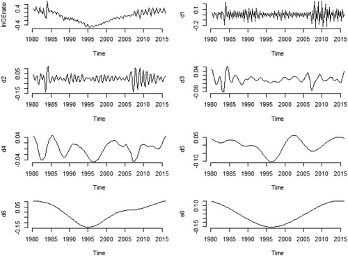
Having explored data properties and the raw-data causal relationships, the causality patterns at different time horizons are investigated using wavelet-decomposed data. The data were deseasonalised prior to the wavelet decomposition, then the wavelet decomposition was done by applying the package Waveslim⁷ in R. Figures 2 and 3 show the time series plots of the wavelet filtered data. The figures clearly show that, at the longer time scales, the oscillations of the time series are longer, that is, the time between consecutive peaks and between consecutive troughs become longer as the time scale becomes larger. The wavelet smooth series representing the trend (s6) illustrates that the trough of both government revenue and expenditure ratio is around 1996, which is also noticeable from the original time series.

Figure 2. Time series plot and wavelet decomposition of the government revenue as a share of GDP.

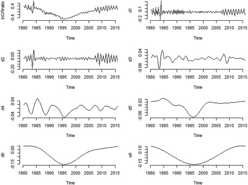
Figure 3. Time series plot and wavelet decomposition of the government expenditure as a share of GDP.

To ensure that the wavelet-filtered series do not have the problem of having a unit root, the five unit root tests were performed again. The results of these are presented in Table 9 below.

Table 9. Unit root test using wavelet filtered data (wavelet details).

Variables	Wavelet scales	ADF	PP	DF-GLS	ERS	KPSS
GR/GDP	1	−5.679***	−44.672***	0.337	26.890	0.192
	2	−3.951***	−16.098***	0.336	5.583	0.092
	3	−3.459***	−2.313	−3.865***	4.581	0.139
	4	−2.435***	−3.155**	−1.699	2.166**	0.109
	5	−1.867**	−1.497	−1.483	6.962	0.236
GE/GDP	1	−5.078***	−89.934***	0.237	11.866	0.045
	2	−4.000***	−17.374***	−0.436	8.005	0.069
	3	−2.646***	0.023**	−1.078	12.289	0.037
	4	−2.875***	−3.170**	−0.915	4.376	0.084
	5	−2.126**	0.337	−1.826	5.365	0.174

Notes: GR/GDP denotes government revenue in log; GE/GDP denotes government expenditure in log. Lags are selected based on the Schwarts information criteria. ***denotes 1% level of significance. ADF, PP, DF-GLS, ERS and KPSS are Augmented Dickey-Fuller test, Phillips-Perron test, Dickey-Fuller Test with GLS Detrending, Elliot, Rothenberg, and Stock Point Optimal (ERS) Test and the Kwiatkowski, Phillips, Schmidt, and Shin (KPSS) Test, respectively. ADF, PP and DF-GLS have null hypothesis is that the series has a unit root while KPSS null hypothesis is that the series is stationary. Barlett kernel is used for PP, ERS and KPSS. The critical values of the tests with constant are presented in Table 3.

Stationarity of the series is more dominantly supported than having a unit root. The DF-GLS and ERS test results generally stand in contrast to the other three tests. Exceptions were found for the wavelet detail series at scale 5 (d5) and 6 (d6) and for the smooth series (s6), which have trend patterns as the original series. Therefore, the Granger causality analysis that follows uses the wavelet detail series, covering time scales from 1 to 4, which are stationary.

For the analysis, at each wavelet scale, Granger causality is tested in both directions between the government revenue and expenditure using the wavelet detail series given in the vector $$y_t\equiv \left[\begin{array}{c}{d}_t^{\hspace{0.17em}\text{ln}\hspace{0.17em}\mathit{GRratio}}\\ d_t^{\hspace{0.17em}\text{ln}\hspace{0.17em}\mathit{GEratio}}\end{array}\right]$$ where $d_t^{\hspace{0.17em}\text{ln}\hspace{0.17em}\mathit{GRratio}}$ and $d_t^{\hspace{0.17em}\text{ln}\hspace{0.17em}\mathit{GEratio}}$ represent the time-t elements of the wavelet detail series for $\text{ln}\hspace{0.17em}\mathit{GRratio}$ and $\text{ln}\hspace{0.17em}\mathit{GEratio}$, respectively.

The vector autoregressive model of order K, VAR(K), as shown below is estimated: $$\left[\begin{array}{c}{d}_t^{\hspace{0.17em}\text{ln}\hspace{0.17em}\mathit{GRratio}}\\ d_t^{\hspace{0.17em}\text{ln}\hspace{0.17em}\mathit{GEratio}}\end{array}\right]=\left[\begin{array}{c}{\beta }_{01}\\ {\beta }_{02}\end{array}\right]+\left[\begin{array}{cc}{\beta }_{11}^{\left(1\right)}& {\beta }_{12}^{\left(1\right)}\\ {\beta }_{21}^{\left(1\right)}& {\beta }_{22}^{\left(1\right)}\end{array}\right]\left[\begin{array}{c}{d}_{t-1}^{\hspace{0.17em}\text{ln}\hspace{0.17em}\mathit{GRratio}}\\ d_{t-1}^{\hspace{0.17em}\text{ln}\hspace{0.17em}\mathit{GEratio}}\end{array}\right]+\cdots +\left[\begin{array}{cc}{\beta }_{11}^{\left(K\right)}& {\beta }_{12}^{\left(K\right)}\\ {\beta }_{21}^{\left(K\right)}& {\beta }_{22}^{\left(K\right)}\end{array}\right]\left[\begin{array}{c}{d}_{t-K}^{\hspace{0.17em}\text{ln}\hspace{0.17em}\mathit{GRratio}}\\ d_{t-K}^{\hspace{0.17em}\text{ln}\hspace{0.17em}\mathit{GEratio}}\end{array}\right]+\left[\begin{array}{c}{u}_{1t}\\ u_{2t}\end{array}\right],$$ where the various β parameters are constants and [u_1t u_2t]´ is the error vector at time t. To investigate whether government expenditure Granger-causes government revenue, whether the hypothesis that all ${\beta }_{12}^{(k)}$ parameters are zero can be statistically rejected should be tested. Similarly, to investigate whether government revenue Granger-causes government expenditure, whether the hypothesis that all ${\beta }_{21}^{(k)}$ parameters are zero can be statistically rejected, should be tested.

The number of lags of the regression models, K, is decided using the Schwarz (1978) information criterion (SIC), the Hannan and Quinn (1979) criterion (HQ), and the Akaike (1971) information criterion (AIC), along with testing for autocorrelation using the multivariate Rao F-test developed by Edgerton and Shukur (1999). The order of the VAR is first determined using SIC, and the test for autocorrelation was done. If any significant autocorrelation is detected, the lag suggested by HQ is used, and the test for autocorrelation is done again. If any significant autocorrelation remains, the AIC is used. Further diagnostic checking continued with the VAR model. If the AIC-suggested lag is used, additional testing for autocorrelation is performed. The Breusch-Godfrey LM test for generalised autoregressive conditional heteroskedasticity (GARCH) effects and the Jarque and Bera (1987) test for non-normality are used to check for GARCH effects and non-normality. The misspecification tests indicate non-normality in almost every case. Therefore, the heteroscedasticity-consistent estimation of the covariance matrix of the coefficient estimates in regression models was used. The Granger causality test results between government revenue and expenditure using wavelet detail series are shown in Table 10.

Table 10. Granger causality test results using wavelet details.

Hypothesis	Wavelet scales (lag length)	F-statistic	Prob.
GE $\nrightarrow$ GR	1 (7)	0.25788	0.9693
GR $\nrightarrow$ GE		0.83694	0.5576
GE $\nrightarrow$ GR	2 (14)	1.4213	0.1455
GR $\to$ GE		3.623	2.268e-05
GE $\nrightarrow$ GR	3 (7)	0.98684	0.4413
GR $\nrightarrow$ GE		1.5679	0.1455
GE $\to$ GR	4 (8)	3.2217	0.0017
GR $\to$ GE		2.8518	0.0048

Notes: GR denotes government revenue ratio to GDP in log and GE denotes government expenditure ratio to GDP in log.

Examining the results at the very finest time scale, the one- and two-quarter wavelet scale (d1), no statistically significant causal relationship between government revenue and expenditure is found. When analysing the results at the next finest time scale, the two- and four-quarter wavelet scale (d2), however, the causality tests show that there is a unidirectional causality running from government revenue to expenditure for China. The causal relationship from revenues to expenditure for up to a year would be partly due to the Chinese budgetary reforms that have been undertaken since 1978 when China adopted the policy of ‘reform and opening’ and intensively after 1994 with the start of the Chinese Budgetary Law. All these series of reforms were intended to establish a more transparent and efficient budgetary system. The implementation of these reform measures has come to some fruition in laying down groundwork for a modern budget system, such as having the government-affiliated departments submit annual budgets to the legislative body, which is a new practice that did not previously exist (Wang 1997). The causal relationship between the revenues and expenditure in a year cycle still does not mean that the budgets would be balanced. Consistent with Friedman (1978), this causal relationship suggests that increasing taxes does not lead to the desired decrease in the budget deficit. Without decreasing budget deficits, the government net debt would accumulate. As mentioned in the previous section, a government budget deficit for a prolonged period of time poses economic problems in terms of interest rate increases and their negative effects on long-run economic growth. This would be relevant to the changing causal relationships of the revenues and expenditure in larger time scales. Although at the four-to-eight-quarter time scales (d3), the inconclusive relationship between the two variables is indicated, in the cycle of the eight- and sixteen-quarter wavelet scale (d4), the presence of bidirectional causality is detected. It implies that, under the cycle of about one to four years, the revenue and spending decisions are made simultaneously after analysing the costs and benefits of alternative government choices, suggesting that government revenue and expenditure help push the budget towards equilibrium (Ho and Huang 2009). This finding of the feedback relationship between government revenue and expenditure in China is in line with the findings of previous studies (Li 2001; Ho and Huang 2009). This bidirectional causal relationship was also found when the Toda-Yamamoto causality test was performed in the current study (Table 8) using the raw data (i.e. before the wavelet analysis). The current study’s causality results based on the wavelet-decomposed data differ from previous studies’ results using the Toda-Yamamoto causality test on the raw data, in that the time scale at which the feedback relationship between these two variables arises can be identified with the help of the wavelet analysis.

6. Concluding remarks and policy implications

In this paper, the causal relationship between government revenue and expenditure for China was examined using quarterly data from 1980–2015. It was first examined whether the two fiscal components have unit roots. The results show very mixed results on having unit roots, even with multiple structural breaks considered in various unit root tests. Detecting different break points of the two nonstationary time series and even finding different orders of integration make the ground for investigating their cointegration relationship unfirm. As a remedy to this problem, along with the economic theories that suggest that the budget decision-making mechanism can vary across various time horizons, the wavelet decomposition is used for studying the causal relationships of the government revenue and expenditure at different time horizons. At the same time, the use of wavelets prevents the problem of nonstationarity (and to some extent, structural breaks). The results indicate that government revenue Granger-causes government expenditure (tax-and-spend hypothesis) in the wavelet scales of two to four quarters and that bidirectional causality (fiscal synchronisation) exists in the wavelet scale of eight to sixteen quarters. These results find some commonalities with the previous country-specific studies on China, which report long-run bidirectional causality (Li 2001; Chang and Ho 2002; Ho and Huang 2009). Compared to the previous studies using traditional time series analysis methods, the current study finds that the causality patterns change over various time horizons for the period of 1980 to 2015 in China. Changes in Granger causality using wavelets are not uncommon due to the feature of unmasking aggregate data at different horizons (Almasri and Shukur 2003; Hacker, Karlsson, and Månsson 2012, 2014, among others). These changes in causal relationships, at different time scales, between government revenue and expenditure in China were not previously documented. Nonetheless, unlike the previous studies, the current study clarifies the cycle when the bidirectional causality is detected. Therefore, this study makes a modest contribution to the empirical literature by empirically analysing the relationship between government revenue and expenditure using Chinese data at various time horizons.

The findings above suggest a number of policy implications. First, the Granger causality result in a year cycle indicates that a unidirectional causality exists in China, running from revenue to expenditure for up to a year cycle. Hence, the policy implication for China is that it should take further steps to broaden its tax base and make further improvements in collecting and administrating revenue, although it has undertaken fiscal reforms over the years. Despite all the improvements, the limitation of these reforms has also been noticed. As mentioned by Deng and Peng (2011), the serious loophole in the Chinese budgetary system in China is that the budget process lacks any budgetary legal authority, which leaves a wide gap between the original budget figures approved by the Chinese legislature (the National People’s Congress) and the final budget. Moreover, substantial changes (additions and subtractions) to the original budget can be made by the government without approval from the legislative body, and expenditure can also be used for other purposes than those approved by the legislature.

The bidirectional causality pattern that was found in a cycle of four years suggests that interdependence between revenues and expenditure must be considered; thus, efforts simply to change either revenue or expenditure would not bring the desired outcome of a decreased budget deficit under the four-year cycle. The simultaneous determination of revenues does not mean that it restrains the budget deficit. If they are related in the same direction, this joint determination of revenue and expenditure still fails to curtail the budget deficit (Dalena and Magazzino 2012).

In summary, to maintain fiscal sustainability, China should have an even more transparent tax system with further discreet tax reforms. While the main purpose of this paper is to offer empirical evidence rather than to suggest a set of salient fiscal policy or budgetary reform measures, the major finding on the causal relationships between government revenue and expenditure at different time scales supports the argument that the budgetary reforms in China have a further way to go for a more transparent and efficient budgetary decision-making system.

Disclosure statement

No potential conflict of interest was reported by the authors.

Additional information

Notes on contributors

Hyunjoo Kim Karlsson

Hyunjoo Kim Karlsson is a senior lecturer in economics at Linnaeus University in Sweden. She received her doctoral degree in economics at Jönköping International Business School, Jönköping University, Sweden, in 2012. Her major area of research is in international economics and finance with a focus on emerging markets. Her recent publications are as below:

- Karlsson, H. K., K. Månsson, and P. Sjölander. 2018. “Investigation of the Nonlinear Behavior in Real Exchange Rates in Developing Regions.” Applied Economics Letters 25 (5): 335–339.

- Karlsson, H. K., Y. Li, and G. Shukur. 2018. “The Causal Nexus between Oil Prices, Interest Rates, and Unemployment in Norway Using Wavelet Methods.” Sustainability 10: 1–15.

- Karlsson, H. K., P. Karlsson, K. Månsson, and S. Pär. 2016. “Wavelet Quantile Analysis of Asymmetric Pricing on the Swedish Power Market.” Empirica 44: 1–12.

- Hacker, R. S., H. K. Karlsson, and K. Månsson. 2014. “The Relationship between Exchange Rates and Interest Rate Differential―A Wavelet Approach.” International Review of Economics and Finance.

- Karlsson, H. K., and S. R. Hacker. 2013. “Time-Varying Sensitivities of Sectoral Returns to Market Returns and Exchange Rate Movements.” Applied Financial Economics 23 (14): 1155–1168.

- Hacker, R. S., H. K. Karlsson, and K. Månsson. 2012. “The Relationship between Exchange Rate and Interest Rate Differential: A Wavelet Approach.” The World Economy 35 (9): 1162–1185.

Notes

1 For example, see Bloomberg (‘China faces biggest fiscal challenge since 1981’, 20 January 2015, at http://www.cnbc.com/2015/01/20/china-faces-biggest-fiscal-challenge-since-1981.html) and ‘China Backpedals on Fiscal Reform – Facing a weakened economy, the government lets borrowing resume’, 28 May 2015, at http://www.bloomberg.com/news/articles/2015-05-28/china-s-local-government-debt-fiscal-reform-reversed).

2 Time scales in a wavelet analysis change on a dyadic basis, which means that $2^j$ denotes a scale, j. This scale is then associated with $2^{j-1}$ to $2^j$ periods. The ‘periods’ in the wavelet scales are related to the data observation frequency. For example, regarding a daily time series, scale 1 means a time scale of 1–2 days. Scales 2 and 3 of the daily series would then mean time scales of 2–4 days and 4–8 days, respectively. Similarly, dealing with monthly data in wavelet analysis makes 1–2, 2–4 and 4–8 months at the time scales of 1, 2 and 3, respectively.

3 Unlike DWT, MODWT has a number of values for the averages at every scale level equal to the number of values in the original series, which is a useful property for our analysis. The wavelet transformation for MODWT is not an orthogonal one, however (Percival and Walden 2000, Ch. 5).

4 Data codes from the database are in the parentheses.

5 The difference between ADF and PP tests should be noted here. While the PP test does not require specific forms of the serial correlations in the data generation under the null hypothesis, the ADF test includes additional higher order lagged terms. This means that, if the autoregressive order is not correctly specified, the test will be either mis-sized or its power will suffer. This problem can be avoided in the PP test. Yet, if the autoregressive order is correctly specified, the PP test will be less powerful than the ADF test (Harris and Sollis 2003).

6 The lag length was decided using the AIC.

7 The R Waveslim package is found at: https://cran.r-project.org/web/packages/waveslim/index.html (2016-07-09).

References

- Afonso, A., and C. Rault. 2009. Budgetary and external imbalances relationship: A panel data diagnostic. CESifo Working Paper No. 2559, CESifo Group Munich.
- Akaike, H. 1971. “Autoregressive Model Fitting for Control.” Annals of the Institute of Statistical Mathematics 23(1): 163–180. doi:10.1007/BF02479221.
- Almasri, A., and G. Shukur. 2003. “An Illustration of the Causality Relation between Government Spending and Revenue Using Wavelet Analysis on Finnish Data.” Journal of Applied Statistics 30(5): 571–584. doi:10.1080/0266476032000053682.
- Athanasenas, A., C. Katrakilidis, and E. Trachanas. 2014. “Government Spending and Revenues in the Greek Economy: Evidence from Nonlinear Cointegration.” Empirica 41(2): 365–376. doi:10.1007/s10663-013-9221-3.
- Baghestani, H., and R. McNown. 1994. “Do Revenues or Expenditures Respond to Budgetary Disequilibria?” Southern Economic Journal 60: 311–322. doi:10.2307/1059979.
- Barro, R. J. 1979. “On the Determination of the Public Debt.” Journal of Political Economy 81: 940–971. doi:10.1086/260807.
- Benhmad, F. 2012. “Modeling Nonlinear Granger Causality between the Oil Price and U.S. dollar: A Wavelet Based Approach.” Economic Modelling 29(4): 1505–1514. doi:10.1016/j.econmod.2012.01.003.
- Brady, G. L., and C. Magazzino. 2019. “Government Expenditures and Revenues in Italy in a Long-Run Perspective.” Journal of Quantitative Economics 17(2): 361. 10.1007/s40953-019-00157-z. doi:10.1007/s40953-019-00157-z.
- Chang, T., and Y. H. Ho. 2002. “A Note on Testing Tax-and-Spend, Spend-and-Tax or Fiscal Synchronization: The Case of China.” Journal of Economic Development 27: 151–160.
- Clemente, J., A. Montañés, and M. Reyes. 1998. “Testing for a Unit Root in Variables with a Double Change in the Mean.” Economics Letters 59(2): 175–182. doi:10.1016/S0165-1765(98)00052-4.
- Crowley, P. 2007. “A Guide to Wavelets for Economists.” Journal of Economic Surveys 21(2): 207–264. doi:10.1111/j.1467-6419.2006.00502.x.
- Dalena, M., and C. Magazzino. 2012. “Public Expenditure and Revenue in Italy, 1862-1993.” Economic Notes 41(3): 145–172. doi:10.1111/j.1468-0300.2012.00243.x.
- Elliott, G., T. J. Rothenberg, and J. H. Stock. 1996. “Efficient Tests for an Autoregressive Unit Root.” Econometrica 64(4): 813–836. doi:10.2307/2171846.
- Deng, S., and J. Peng. 2011. “Reforming the Budgeting Process in China.” OECD Journal on Budgeting 11(1): 75–89. doi:10.1787/budget-11-5kggc0zqj8f0.
- Edgerton, D., and G. Shukur. 1999. “Testing Autocorrelation in a System Wise Perspective.” Econometric Reviews 18(4): 343–386. doi:10.1080/07474939908800351.
- Friedman, M. 1978. “The Limitations of Tax Limitation.” Policy Review, Summer, 7–14.
- Glynn, J., N. Perera, and R. Verma. 2007. “Unit Root Tests and Structural Breaks: A Survey with Applications.” Journal of Quantitative Methods for Economics and Business Administration 3: 63–79.
- Gregory, A. W., and B. E. Hansen. 2009. “Tests for Cointegration in Models with Regime and Trend Shifts.” Oxford Bulletin of Economics and Statistics 58(3): 555–560. doi:10.1111/j.1468-0084.1996.mp58003008.x.