Efficient crash structure design for road traffic accidents of tomorrow

Abstract

Energy absorbing structures (EAS) play a vital role in automotive crash mitigation systems and save countless lives each year. Innovative EAS design ideas such as cross-sectional geometry is an area under intense research as evidenced by a large number of publications in recent years. It is however very difficult to directly compare the efficiency of the design suggestions due to parameter variation. This paper identifies designs with the highest potential, introduces an efficient reduced order modelling methodology and provides the first comprehensive unbiased benchmark. Critical evaluation of results reveal that some designs have inherent issues not previously reported, whilst others demonstrate significant potential for improving EAS performance compared to “conventional” designs.

Keywords:

• Crash structure optimization
• reduced order modelling
• multi-angle crash structures
• multi-cell crash structures
• crash structure benchmarking

1. Introduction

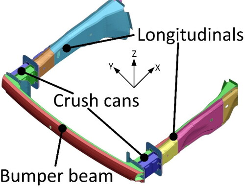
Over the last 60 years front-end automotive crash structure designs have gradually evolved to a ‘conventional’ or ‘industry standard’ setup (Figure 1) comprising of three main components namely the bumper beam, the crush cans for low speed impacts (<2.78 m/s) and the longitudinals for high speed impacts (>2.78 m/s).

Figure 1. Conventional automotive front-end crash structure.

Designed to minimise occupant injuries, the optimal crash performance criteria of a front-end crash structure and its individual components can broadly be described as:

1. Maximising impact Energy Absorbed (EA).

2. Limiting maximum acceleration levels.

3. Eliminating passenger cell intrusion.

The specific front-end crash structure in Figure 1 originates from a mass produced vehicle namely the Ford Fiesta. The YZ-plane cross-sections (Figure 1) of the crush cans and the longitudinals could simplistically be modelled as rectangular or double top-hat sections; despite it being evident that neither cross-section is constant as a function of moving along the X-direction. As an example, the longitudinals must often accommodate the tyre envelope. Consequently, the cross-sectional area is often reduced in the vicinity of the firewall. Nevertheless, such geometry simplifications are frequently done for general comparative studies, [1], as the intricate details of the cross-sectional design is often dictated by packaging requirements e.g. for powertrain, suspension or auxiliary components.

In recent years a multitude of authors, such as [2–4], have proposed a new Innovative Energy Absorbing Design (IEAD) which could e.g. be utilised for bumper beam, crush can or longitudinal applications. In the vast majority of cases authors claim that their proposed IEAD performs significantly better than conventional crash structure designs (e.g. rectangular cross-sections) in terms of the three optimal crash performance criteria listed above. EA is however most often replaced by the Specific Energy Absorbed (SEA). SEA is arguably a more appropriate indicator of crash structure efficiency as it is obtained by dividing the EA with the mass of the crash structure.

A direct comparison of crash performance, i.e. benchmarking, of the vast majority of IEADs is however not possible using the publications in which the individual design was originally proposed. This is because the scenarios investigated to evidence the crash performance of the individual IEAD vary greatly in terms of materials, geometrical dimensions and impact scenario parameters such as speed, angle and mass of the impactor. A simple ‘scaling’ of performance is also not possible due to the inherent complexity and non-linear nature of (high deformation) impact scenarios. Focusing on longitudinal and crush can applications this paper will provide a realistic crash performance benchmark, across a range of impact scenarios, which enables a truly unbiased comparison of competing IEADs relative to each other and ‘conventional’ crash structure designs. Consequently, the individual IEADs realistic potential for improving crash performance can be critically assessed and high yield individual designs and/or design trends identified for future research and development. This is of particular importance in the context of increasing levels of vehicle autonomy, which may lead to dramatic changes in accident scenarios such as impact speed, as well as significant changes to powertrain configurations, which in turn may lead to substantial changes in the geometrical design space for crash structures. This paper will also address significant shortcomings, limitations and oversights in relation to the crash performance stated by authors in the publications wherein individual IEADs were originally proposed as shall be subsequently discussed.

2. Literature review

As stated in the introduction front-end automotive crash structure designs have been continuously developed and refined since the 1960s. At present the prevailing cross-sectional geometry (YZ-plane, Figure 1) of the vast majority of longitudinals and crush cans manufactured can simplistically be modelled as double top-hat or rectangular. There may be many different reasons for this preference, the most likely reasons include the simplicity of manufacturing, relatively low structural mass, the consistency/robustness of crash performance as well as limitations and uniformity of most design volumes (packaging space). Hence, from a multi-objective perspective it is likely that these conventional cross-sections are effectively the optimum or best compromise solution for most applications. Emerging trends in other areas are however likely to increasingly question the optimality of conventional designs and consequently necessitate the exploration of IEADs. For example, the introduction of Connected Autonomous Vehicle (CAV) technology is highly likely to significantly change front-impact scenarios; e.g. angle and speed, whilst impending changes to powertrains may significantly alter the packaging space and crumple zone dimensions at the front-end of a vehicle. With this in mind newly proposed IEADs become increasingly relevant for exploration. In the preparation of this paper in excess of 40 recently published journal papers have been reviewed with key observations discussed below. Due to conciseness, it is not possible to explicitly discuss all papers in this manuscript; a full bibliography is available upon request. As a starting point IEADs will be divided into separate categories based on the type of innovation proposed: functional grading and cross-sectional geometry.

2.1. Functional grading

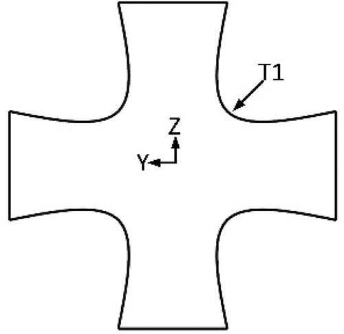
Throughout this paper the term Functional Grading (FG) refers to the variation of a specific attribute along a given direction, i.e. X, Y or Z in Figure 1. FG may be further divided into three sub-categories; Material (FG-M), Thickness (FG-T) and Shape Variations (FG-SV), examples of all three are illustrated in Figure 2.

Figure 2. Examples of functional grading.

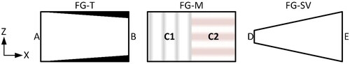
Figure 2 (FG-T) illustrates how the wall thickness of a component increases along the X-axis from A to B (grossly exaggerated). FG-M in Figure 2 demonstrates a component made from two different (composite) materials C1 and C2. Please note that the total thickness of C1 and C2 may be identical or vary, C1 and C2 may be made from identical plies but with different orientations and/or thickness’. Furthermore, the transition from C1 to C2 may be gradual as opposed to the distinct divide illustrated in Figure 2. Also note that foam and honey-comb filler materials will be included in this category. Nevertheless, the emphasis will remain on ‘advanced’ FG-M applications wherein more than one material property change occurs.

FG-SV in Figure 2 illustrates FG in terms of ‘dramatic’ but linear shape changes; in this case a significant taper. Note that the linear shape changes occurs along the X-axis of the component (Figures 1 and 2). Please also note that for the remaining discussions in this paper the directions and axes referenced will utilise the co-ordinate systems defined in Figures 1 and 2; i.e. the cross-sectional geometry will refer to the YZ-plane and the longitudinal (or axial) direction refers to the X-axis.

Table 1 provides a summary of the reviewed papers wherein FG was used to improve the energy absorbance capabilities of IEADs. Table 1 contains an overview of the type of FG used (as defined in Figure 2), the type of loading applied and the SEA improvement obtained by the IEAD relative to a reference structure which in some cases relate to pre and post IEAD optimisation whilst in other instances it refers to a ‘conventional’ non FG structure such as a square tube.

Table 1. Overview of functional grading (FG) literature review results.

Paper #	FG			Loading		Max claimed SEA improvement relative to ‘reference’ structure
	M	T	SV	Axial	Bending
[2]			Y	Y		107%
[3]			Y	Y		No reference structure
[4]		Y	Y	Y		100%
[5]		Y		Y		20%
[6]		Y		Y		83%
[7]		Y		Y		35%
[8]		Y		Y		54%
[9]		Y		Y	Y	17%
[10]		Y		Y		27%
[11]	Y	Y		Y		15%
[12]	Y			Y		No reference structure
[13]	Y			Y		35%
[14]	Y			Y		45%
[15]	Y			Y		No reference structure
Average (FG-M/FG-T/FG-SV/Total):						31%/44%/103%/49%

As indicated in Table 1, the most prevalent form of loading used is axial representative of longitudinal and crush can loading in general. The papers, which utilise axial loading, contain at least one load scenario wherein the impactor travels along the axial/longitudinal direction of the IEADs, i.e. the X-axis in Figure 1.

Table 1 also reveals that the main emphasis is on FG-T; it should be noted that all papers reviewed utilise isotropic materials, i.e. metallic. The last column in Table 1 contains the maximum improvement claimed by individual authors as a ratio of SEA of the proposed IEADs and the SEA of a reference structure. Although the calculations from individual papers are not directly comparable, as discussed in the introduction, the numbers do provide an indication of the magnitude of improvements, which can be expected. In this context, it should also be noted that the average SEA improvements are calculated on results from a limited and varying number of research papers. With this in mind, Table 1 indicates that, by utilising FG the SEA can be improved by 49% on average.

FG-SV provides the highest average improvement of 103%, this is however only based on results from papers [1, 4] as no other relevant papers were found. Note that a third paper [3] also contains FG-SV, but it does not state an explicit improvement on SEA in relation to a reference structure. [1, 3] are the only papers which only contain FG-SV whereas [4] considers FG-T as in combination with FG-SV. [1] contains the highest claimed FG-SV based SEA improvement of 107%; the paper investigates the structural performance of empty and foam filled conical thin walled aluminium tubes similar to the FG-SV illustration in Figure 2. The structure was exposed to impacts at various angles between 0° and 30° (relative to the X-axis). Please note the mass of the impactor is not defined in the paper. The FG-SV consists of varying the angle of the cone; i.e. the slope in the X-direction. This approach is very similar to the lowest FG-SV based SEA improvement of [4] which also used a conical tube of the same dimensions as in [1] but at a higher impact speed. The maximum SEA improvement (of 100%) in [4] was found at an impact angle of 20 degrees; for the 0 degree impact; i.e. at the same angle as in [1] the SEA improvement was found to be 68%. Additional details of the IEAD dimensions and external loading for the highest and lowest SEA improvements for FG-SV ([1, 4]), FG-T ([6, 11]) and FG-M [13,14]) are listed in Table 2.

Table 2. Details of highest and lowest FG based SEA improvements.

Paper #	IEAD dimensions (mm)			External load
	X	Y	Z	Speed (m/s)	Mass (kg)
[1]	200	80	80	10
[4]	200	80	80	15	90
[6]	180	50	50	1	N/A
[11]	240	80	80	15	600
[14]	250	80	80	10	N/A
[13]	200	60	60	20	600

Compared to [1] and [3,4] uses a 50% longer tapered steel structure of 300 mm (X) with a square cross-section (YZ-plane) of approximately 50 mm (end E of the FG-SV illustration in Figure 2) and 35 mm at end D. This structure was impacted at 15 m/s with a mass of 480 kg. The comparison of the loading scenarios in [1, 3] and [4] clearly underlines the difficulty of directly comparing results of different IEADs as discussed in the introduction.

FG-T provides the second highest average SEA improvement of 44% with individual results ranging from 15% to 100%. These are based on the results from eight papers including [4, 11] that consider a combination of FG-T/FG-SV and FG-T/FG-M respectively. Notably, the highest and lowest SEA improvements are claimed in these ‘combination’ studies. Excluding the combined study in [4] the highest SEA improvement of a purely FG-T based study is 83% from [6]. |This paper explored FG-T optimisation of square thin walled tubes by varying the thickness along the X direction using displacement controlled experiments.

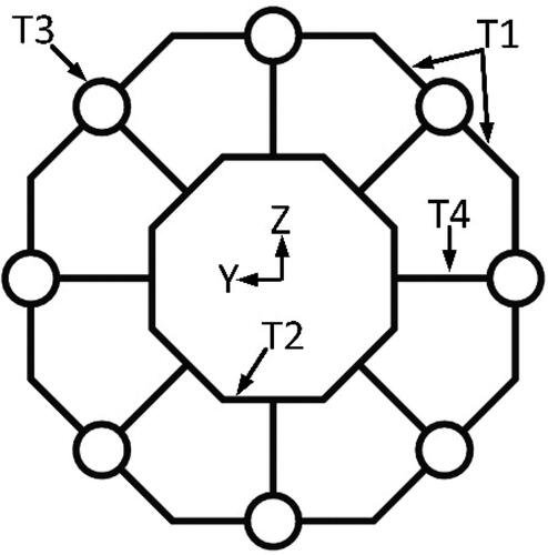
The lowest FG-T based SEA increase of 15% originates from [11] which combined FG-T and FG-M as illustrated in Figure 3.

Figure 3. YZ-cross section from [11].

FG-T was achieved by varying the thickness of the outer (metallic) shell, illustrated as layer 1 in Figure 3 with the thickness remaining constant throughout the length (i.e. X-direction). Layers 2, 3 and 4 represent foam filler materials. The density of the foam was varied throughout the layers (in the YZ-plane only) and it was determined that a descending density (from layer 2 through layer 3 to layer 4) provided the most optimal crush performance. Please note Figure 3 is a simplified model; the actual model used in [11] contained a total of 26 foam layers. The info in Table 2 may suggest that [11] has a distinct disadvantage in the load speed in addition to a significant increase in length (X-dimension) which could lead to instabilities unless mass is added e.g. through wall thickness with the likely consequence of reduced SEA improvement. It is however also difficult to directly compare results due to the parameter variations between the two studies.

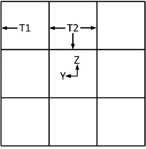
FG-M provides the lowest average SEA improvement of 31% (Table 1) with individual results ranging from 15% to 45% based on only 4 papers. The lowest improvement of 15% is the same study as in the FG-T section; i.e. [11]. The lowest FG-M only based SEA improvement was found in [13]; which explored the influence of different fill patterns and filler materials upon SEA using a rectangular cross-section as illustrated in Figure 4.

Figure 4. Cross-sectional geometry from [13].

FG-M was explored through 13 different fill patterns using the five distinct areas illustrated in Figure 4 with different foams and/or honeycomb materials. [13] concluded that the best filling method is to use foam in sections 1–4 and honeycomb in section 5. The paper also concluded that filler materials may have an adverse effect upon SEA using certain fill patterns. This is also identified in [15] wherein an ‘empty’ thin walled conical tube (FG-SV) was determined to perform better than its foam-filled counterpart.

The highest FG-M based SEA improvement was found in [14]; which explored hollow and foam filled tubes of varying cross-sections including square, rectangular, elliptic and circular. Using displacement controlled experiments the loading was applied at angles between 0° and 30° relative to the X-axis. The highest SEA improvement was obtained using a foam-filled thin walled tube with an elliptical cross-section. Although not explicitly discussed above, a number of research papers, e.g. [1], identify and explore auxetic foams, i.e. foams with negative Poisson’s ratio, as being particularly effective for energy absorbing structures (FG-M) including longitudinal and crush can applications.

Based on the papers reviewed FG seemingly has a positive effect on SEA; however the significant variation of specimen dimensions, cross-sectional geometry, material, impact direction and load magnitudes prohibit direct and explicit comparison of results.

2.2. Cross-sectional geometry

The cross-sectional geometry undoubtedly has a significant effect upon the crash performance of longitudinals and crush cans and has been the focus of countless investigations. Although many of the papers discussed in section 2.1 also explored different cross-sections many of these were however ‘conventional’ if the FG aspects are ignored. Recent cross-sectional geometry based research efforts have particularly focused on multi-cell and multi-corner designs, in this section a handful of carefully selected results of particular relevance and importance will be discussed. The basic principle of multi-cell structures is simply to divide the cross-section into multiple segments (or cells). The multi-cell structure illustrated in Figure 5 was deemed to be most efficient in increasing SEA in [14] in combination with FG-M as discussed in the previous section.

Figure 5. 9-cell (multi-cell) structure: SQ9.

[14] concluded that the nine cell structure illustrated in Figure 5 consistently performed significantly better (in terms of SEA) than a range of other cell division including a simple square cross-section. There are many other examples of research into multi-cell structures including [3, 16].

[16] explored square and circular cross-sections and concluded that the best structural performance was achieved with a five cell square section with rounded corners subject to displacement controlled experiments at 0.1 m/s. [3] explored the effects of triangular, square, hexagonal and octagonal cross-sections with up to four internal cells also subject to displacement controlled load applied at 1.6E-4 m/s. The paper concluded that hexagonal and octagonal cross-sections where the internal cells meet the outer walls at the mid-points, as opposed to where the outer side-lengths join, were the most effective. These achieved an SEA increase up to 120% in relation to a reference square cross-sectional structure. A 4-cell octagonal cross-section with mid-point inner cell connections is illustrated in Figure 6.

Figure 6. Octagonal cross-sections: Octa_8 (left), Octa_4 (centre), Octa_0 (right).

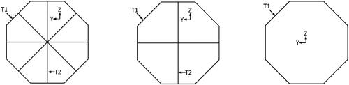
The identification of the mid-point cell connection is in agreement with the conclusions of [17] which focused on optimisation of multi-cell hexagonal tubes.

In addition to being a multi-cell structure the cross-section illustrated in Figure 6 is also an example of a multi-corner cross-section which have generally been explored as viable options for significantly improving energy absorbance capabilities in comparison to ‘conventional’ cross-sections. [18] also explored multi-cell and multi-corner cross sections determining that a 12-cell dodecagon had a significantly higher energy absorbance (SEA was not used) in comparison with a range of primarily multi-corner cross sections subject to displacement controlled loading.

The highest SEA improvement found throughout the literature review was 145% [19]. This was achieved by utilising a multi-cornered section entitled Criss-Cross tube connected through SPLines (CCSPL) as illustrated in Figure 7.

Figure 7. CCSPL cross-section.

Further exploration of multi-cell and multi-corner cross-sections include refinements obtained via bio-inspired designs. Based on quadrilateral, hexagonal and octagonal sections [20] created a number of Bionic Multi-Cell Tubes (BMCT) inspired by the microstructure of beetle forewings. The energy absorbance of different BMCTs were compared to each other based on a displacement controlled loading scenario. The paper concluded that the most efficient design used octagonal inner and outer sections connected at mid-points, in-line with the conclusion of [3]. The optimised BMCT cross-section is illustrated in Figure 8.

Figure 8. BMCT cross-section.

Table 3 provides a comparative overview of the above discussed results obtained by other authors in relation to improving SEA through cross-sectional geometry variations.

Table 3. Overview of cross-section literature review results.

Paper #	Maximum external dimensions (mm)			Optimal cross-sectional geometry determined	External load		Max claimed SEA improvement relative to ‘reference’ structure
	X	Y	Z		Speed (m/s)	Mass (kg)
[14]	200	80	80	9-cell square	15	600	25%
[16]	120	36	36	5-cell square with rounded corners	0.1	N/A	18%
[3]	70	60	60	Hexagonal and octagonal multi-cell	1.6E-4	N/A	120% (hexagonal) 118% (Octagonal)
[17]	180	72	72	Hexagonal with web-to-web	15	600	SEA not calculated
[18]	500	120	120	12-cell dodecagon	1	N/A	SEA not calculated
[19]	200	75	75	Criss-cross connected through splines	1		145%
[20]	240	100	100	Octagonal bionic multi-cell tube	10	N/A	No reference structure
Average:							85%

By comparing Tables 3 to 2 the previously discussed variation of parameters between different publications is evident. For example, lengths (X-direction) range from 70 mm to 500 mm, cross-sectional dimensions (YZ-plane) range from 36 mm to 120 mm and mass of impactors (where applicable and identified) range from 90 kg to 600 kg at impact speeds of 1.6E-4 m/s to 20 m/s. These variations make a direct comparison (benchmark) of results impossible. It should also be noted that some authors utilised displacement controlled (numerical) experiments, which in combination with a strain rate independent material, makes the impact speed irrelevant in terms of results variation. This is however not consistently the case across all papers reviewed. Comparing Tables 3 to 1 suggests that on average the use of FG improves the SEA by 54% whilst variations of cross-sectional geometry including multi-cell and multi-angle variations leads to an average improvement of 85%. The statistical confidence of these numbers is very low partially due to additional parameter variations. In addition to the different number of papers included in Tables 3 and 1, each paper has a different reference point, or benchmark, for which the SEA improvements are calculated; e.g. different geometrical dimensions and/or loading conditions. As previously discussed, these variations make direct comparison of performance and potential for real world crash applications impossible.

3. Methodology

This section outlines the methodology which will be used to create a benchmark for an unbiased and direct comparison of IEADs specifically to evaluate the real world potential for crush can and longitudinal applications. The section will firstly cover the important crash parameters, followed by the numerical model definitions, optimisation setup and finally an overview of individual case studies.

3.1. Crash performance parameters

In terms of occupant injuries and fatalities the most severe automotive accident in general is a frontal collision [21]. The front crush can and longitudinals are designed to reduce occupant injuries by absorbing as much impact energy as possible, limiting maximum acceleration levels transferred to occupants and eliminating passenger cell intrusions. The crash performance of a crush can and/or longitudinal can therefore be assessed by measuring the deformation EA, peak acceleration levels and associated duration as well as maximum displacement levels of the structure during the impact. The EA is often extended to SEA thereby providing an energy per unit mass measurement. The relevance of these parameters are well established and have generally been used throughout the reviewed papers. It should however be noted that the peak acceleration magnitudes can be significantly influenced e.g. by the introduction of crush initiators designed to ‘guide’ the deformation at the initial stages of the impact. Crush initiators can also significantly influence the Peak Crush Force (PCF) which is often used as a measure of structural stability during the (initial) stages of an impact. Excessive PCF levels may lead to a sudden collapse or buckling of the structure drastically reducing the EA. Hence, the acceleration and peak force magnitudes should be taken as guideline values rather than absolute values more so than the SEA and displacement magnitudes.

A significant shortcoming and limitation of the vast majority of papers reviewed has however been the complete disregard for the backup structure. Consequently, it is assumed that the backup structure to which the crush can or longitudinal is attached is infinitely rigid. This is of course not the case for real world applications; therefore the rigidity of the backup structure must be considered by limiting the force transferred. The crash performance parameters, including targets to indicate optimal crash performance are summarised in Table 4.

Table 4. Crash performance parameters.

Parameter	Acronym	Units	Target
Specific Energy Absorbed	SEA	J/kg	Maximise
Peak Acceleration magnitude	PA	mm/s^2	Limit
Peak Crush Force magnitude	PCF	N	Limit
Displacement (X,Y,Z) magnitude	DX, DY, DZ	mm	Limit
Backup Structure Load Magnitude	BSLM	N	Limit

3.2. Case study overview

As previously mentioned, the overall purpose of this paper is to critically assess, evaluate and compare the crashworthiness performance of recently proposed IEADs using an unbiased and consistent benchmark. As the main focus of attention is longitudinals and crush cans it was decided to fully constrain the test specimen (IEAD) at one end (B) whilst subjecting it to an impact load, travelling in the X-axis direction at the other end (A), as illustrated in the left hand side of Figure 9.

Figure 9. Test setup.

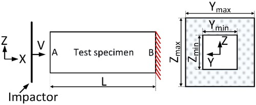
The severity of crash scenarios is heavily dependent upon impact speed which consequently is considered during the case study. Given that approximately 1,500 FE models were expected for the case study a prescribed displacement (and constant velocity) approach was selected over initial velocity thus eliminating concerns about premature termination or excessive CPU consumption (run time).

Specifically, the external loading constitutes an impactor of mass m travelling at a constant velocity of V perpendicular to the longitudinal (X) direction. The maximum (X) displacement of the impactor is equal to 99% of L (Figure 9) and the crush speed will be controlled by adjusting the time it takes the impactor to reach the maximum displacement value. Although this approach does not determine if the test specimen can absorb all impact energy; i.e. determine if the velocity of the rigid wall reaches zero, it provides a useful and unbiased means of comparing IEADs.

As discussed in section 2, results suggest that FG can significantly improve SEA. Based on those discussions, including the summary in Table 1, indications are that FG-SV is the most influential variation of FG. Additionally, it could also be argued that FG-T and FG-M can be completed subsequent to FG-SV. Furthermore, FG-M may have a detrimental effect on SEA and general crash performance. It was therefore decided to only implement FG-SV in the subsequent case study. This will be done by independently varying the cross-sectional dimensions at end (A) and (B) in intervals between Y_min and Y_max as well as Z_min and Z_max as illustrated on the right hand side of Figure 9. Please note the aspect ratios of the cross-sections in a given end (i.e. A or B) will be retained, i.e. Z equals Y. Furthermore, as FG-T is not included in this study the FG-SV can be controlled through variation of two parameters YZA (end A Figure 9) and YZB (end B). YZA and YZB thus represent the external dimensions of the given cross-section with the material thickness controlled through the parameters (design variables) listed in Table 5. As FG-T is not included the thickness will remain uniform throughout the length; i.e. x-direction, Figure 9.

Table 5. Cross-sections for case study.

Name	Illustration	Design variable
		ID	Description
BMCT	Figure 8	T1	Outer octagon thickness
		T2	Inner octagon thickness
		T3	Tube thickness
		T4	Web thickness
CCSPL	Figure 7	T1	CCSPL thickness
Dodecagon	Figure 10	T1	Outer dodecagon thickness
		T2	Inner dodecagon thickness
		T3	Web thickness
Hexa-0		T1	Hexagon thickness
Hexa-3 Hexa_6		T1	Hexagon thickness
		T2	Web thickness
Octa-0	Figure 6	T1	Octagon thickness
Octa-4 Octa-8		T1	Octagon thickness
		T2	Web thickness
RS	Figure 10	T1	Rounded square thickness
		T2	Web thickness
SQ		T1	Square thickness
SQ-9	See Figure 5	T1	Square thickness
		T2	Web thickness

Based on the literature review a total of twelve different cross-sectional designs were chosen for the case study. Consequently, the cross-sections are selected based upon results from multiple comparative studies and should therefore have the highest potential for optimal crash performance including maximum SEA. It should also be noted that some of the cross-sections originate from studies which include parameters not included in the current case study such as FG-T. The twelve cross-sections including identification of thickness variables are defined in Table 5, with Figure 10 showing previoulsy unillustrated cross-sections.

Figure 10. From top left: Dodecagon, RS, SQ, Hexa_0, Hexa_3 and Hexa_6.

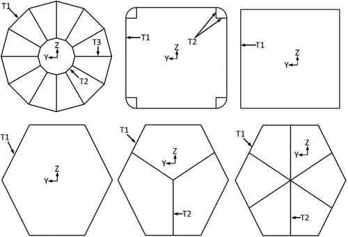
In Table 5 SQ represents the ‘benchmark,’ the CCSPL, Octa_0 and Hexa_0 represent multi-corner cross-sections whilst the remaining cross-sections are multi-cell.

Based on ‘typical’ real world crash structures a set of optimisation parameter values and constraints have been defined as listed in Table 6.

Table 6. Fixed parameters for all subsequent studies.

Parameter	Value(s)
YZA YZB (Figure 9)	Min: 75 mm	Max: 150 mm
Ti (Table 5)	Min: 0.1 mm	Max: 4 mm
Maximum X-displacement magnitude	0.99 * L
Maximum Y and Z-displacement magnitude	20mm
Mass of impactor	684kg
Objective	Maximise SEA

In relation to the parameters listed in Table 6 it should be noted that:

• The range for all thickness design variables (T_i) defined in Table 5 are identical.

• Y and Z displacement constraints are applied to filter out infeasible results and configurations; e.g. structures exhibiting buckling or other sudden collapse.

• The mass of the impactor is fixed at 684kg representing half the mass of a mid-sized vehicle.

• PCF has not been used as a constraint. This is because PCF can be reduced through the introduction of e.g. crash initiators (as is the case with the acceleration). Furthermore, the load transferred to the backup structure will be subsequently defined can be considered representative of PCF.

The acceleration magnitude (in ‘g’) is measured on the rigid wall (impactor Figure 9), and calculated as defined in equation (1)(1) $$\mathit{Acceleration}=\mathrm{ }\frac{{\left(\mathit{Rigid}\mathrm{ }\mathit{wall}\mathrm{ }\mathit{energy}\right)}_{\mathit{CFC}600}}{9.81\frac{mm}{s^2}·684kg}$$(1) . (1) $$\mathit{Acceleration}=\mathrm{ }\frac{{\left(\mathit{Rigid}\mathrm{ }\mathit{wall}\mathrm{ }\mathit{energy}\right)}_{\mathit{CFC}600}}{9.81\frac{mm}{s^2}·684kg}$$(1)

In crashworthiness applications, signals are filtered following the J211 protocol [22]; accelerations can been filtered using a 4 pole Butterworth Channel Frequency Class (CFC) at 180 Hz or 600 Hz. The CFC600 in equation 1(1) $$\mathit{Acceleration}=\mathrm{ }\frac{{\left(\mathit{Rigid}\mathrm{ }\mathit{wall}\mathrm{ }\mathit{energy}\right)}_{\mathit{CFC}600}}{9.81\frac{mm}{s^2}·684kg}$$(1) indicates that a 600 Hz signal filter was applied to the rigid wall energy curve in order to reduce numerical noise of the results. This particular filter was chosen based on a series of pilot studies completed prior to the case study of this paper.

For clarity the SEA was calculated as specified in equation 2(2) $$S\mathrm{E}A=\mathrm{ }\frac{\underset{t=0}{\overset{t=\mathit{tend}}{\int }}\mathit{Internal}\mathrm{ }\mathit{energy}}{\mathit{mass}\mathrm{ }of\mathrm{ }\mathit{test}\mathrm{ }\mathit{specimen}}$$(2) , where internal energy refers to the deformation energy stored in the test specimen and t_end refers to the final step of the simulation: (2) $$S\mathrm{E}A=\mathrm{ }\frac{\underset{t=0}{\overset{t=\mathit{tend}}{\int }}\mathit{Internal}\mathrm{ }\mathit{energy}}{\mathit{mass}\mathrm{ }of\mathrm{ }\mathit{test}\mathrm{ }\mathit{specimen}}$$(2)

The case study in this paper consists of 6 optimisation studies covering a mixture of impact speed (V), test specimen length (L) and design variables as defined in Table 7. Note that each of the 6 studies listed in Table 7 will be conducted for each of the 12 cross-sections defined in Table 5.

Table 7. Optimisation study definitions.

Study	Impact velocity (m/s)	L (mm)	Optimisation design variables
			Name	Min (mm)	Max (mm)	Increment (mm)
A	2.78	200	Ti	0.1	4.0	0.1
			YZA = YZB	75.0		N/A
B	15	400	Ti	0.1	4.0	0.1
			YZA = YZB	75.0		N/A
C	2.78	200	Ti	1.0		N/A
			YZA & YZB	75.0	150.0	0.1
D	15	400	Ti	1.0		N/A
			YZA & YZB	75.0	150.0	0.1
E	2.78	200	Ti	0.1	4.0	0.1
			YZA & YZB	75.0	150.0	0.1
F	15	400	Ti	0.1	4.0	0.1
			YZA & YZB	75.0	150.0	0.1

Note that only one impact angle representing a head-on collision (0°) was chosen, this is because the stand-alone IEAD will be most efficient at this angle. The two initial impact speeds represent low and high speed impacts at 2.78 m/s (10 km/h) and 15 m/s (54 km/h) respectively. The test specimen dimensions including the two lengths of 200 mm and 400 mm were chosen, as they are representative of real-world crash structure dimensions. It should be noted that all studies which include a V of 2.78 m/s also have a specimen length L of 200 mm; these can thus be considered to represent the crush cans (Figure 1). In an analogue manner if V equals 15 m/s L equals 400 mm and can thus be considered to represent the longitudinals (Figure 1).

In accordance with most other studies the main objective of all optimisation studies in this paper is to maximise SEA. Unlike most other studies each of the 6 optimisation studies defined in Table 7 will be completed with and without consideration for the rigidity of the backup structure in combination with an upper acceleration limit. To distinguish between the three setups the suffix ‘_IR’ will be added where an Infinitely Rigid backup structure is considered (e.g. A_IR). ‘_IR_40’ is identical to ‘_IR’ but with the addition of a 40 g acceleration constraint (e.g. A_IR_40) whereas ‘_LLM’ indicates that a Limited Load Magnitude backup structure (e.g. A_LLM) is considered. In the ‘_LLM’ studies an additional optimisation constraint entitled Back-up Structure Load Magnitude (BSLM) will be implemented. The BSLM will be calculated by summation of force magnitudes across all Single Point Constraint (SPC) locations (Figure 9) as defined in equation 3(3) $$\mathit{BSLM}=\sum _{i=1}^{i=N_{\mathit{SPC}}}{\mathit{FSPC}}_i$$(3) : (3) $$\mathit{BSLM}=\sum _{i=1}^{i=N_{\mathit{SPC}}}{\mathit{FSPC}}_i$$(3)

In (2) N_SPC refers to the number of SPCs and FSPC_i refers to the force magnitude for the individual SPC node. Two distinct BSLM limits will be implemented in the relevant _LLM optimisation studies. As discussed above, the studies listed in Table 7 represent either the crush cans or longitudinals (as a function of V and L). It is therefore appropriate to define two distinct BSLM limits, Table 8.

Table 8. BSLM constraint definition for _LLM optimisation studies.

V	L	Maximum BSLM
2.78 m/s	200 mm	80 kN
15 m/s	400 mm	200 kN

The values listed in Table 8 are based on the load magnitudes that ‘typical’ automotive backup structures can absorb before experiencing significant deformation. To clarify, study A_LLM will have a BSLM constraint of 80 kN applied, whereas B_LLM will have a BSLM constraint of 200 kN applied etc.

The variations between the three optimisation setups are defined in Table 9 where Y and N indicates the inclusion or exclusion of a given constraint respectively.

Table 9. Optimisation constraints.

Constraint	Prefix
	LLM	IR_40	IR
Maximum acceleration magnitude = 392 m/s^2 (∼40′g’)	Y	Y	N
Maximum BSLM limit (Table 8)	Y	N	N

The _LLM study is the most constrained study and provides an overview of the IEADs’ ‘natural’ ability to meet the relevant constraints. The _IR study is an unconstrained study which purely explores the IEADs’ SEA potential. This is relevant as parameters including peak acceleration levels can be significantly influenced by the introduction of e.g. crash initiators as previously discussed. The IR_40 setup is included as a pilot study found the BSLM constraint to be the most dominant in general (i.e. most difficult to meet) whilst the acceleration constraint could be met in many cases.

The case study thus consists of 18 studies (A-F with _LLM, IR_40 and _IR variations). By comparing the results of these trends can be identified into the effects of different parameters upon the structural performance.

In general studies A_IR and B_IR can be considered to provide the first benchmark providing an unbiased direct comparison of the 12 different IEADs defined in Table 5 including the ‘standard’ SQ cross-section varying only the wall thickness. Studies A_IR_40, A_LLM, B_IR_40 and B_LLM will explore to what level the consideration of backup structure influences the crash performance and structural efficiency.

Studies C and D (_IR, IR_40 as well as _LLM) can also be considered to provide a first benchmark, but this time with an emphasis on FG-SV in isolation (fixed unity wall thickness).

Studies E and F provides the first benchmark overview of the combined effects of cross-sectional geometry, wall thickness as well as FG-SV with and without consideration for the back-up structure.

The comparison of individual studies will be further discussed in the results section. The next section defines the numerical models used for the optimisation studies.

3.3. Numerical model setup

Explicit LS-DYNA based FE models were developed for the purpose of completing the optimisation studies. The general models were setup as illustrated in Figure 9, with the impactor modelled as a rigid wall. Additional FE parameters are listed in Table 10.

Table 10. Additional FE model parameters.

Parameter	Value
Element size	2.0 mm
Element Type	Shell
Element formulation	Belytschko-Tsay
Element Integration points	5
Contact	Automatic single surface
Static/Dynamic contact friction	0.2
Material Model	Elasto-plastic
Element Thickness	See Table 7

A series of mesh convergency studies were completed in order to determine an appropriate element size across all models and cross-sections. The convergency studies included considerations for the impending FG-SV which was implemented by introducing morphing within individual models as illustrated by the BMCT cross-section in Figure 11.

Figure 11. Morphing end A (left), no morph/morph end A and B (centre), morph end B (right).

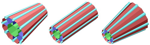
Note that the morphing handles are located at both ends of the structure, i.e. location A and B (FG-SV, Figure 2) and that the cross-section ratios remain constant, as previously defined. Finally, it should also be noted that either end can morph by an identical amount effectively removing the FG-SV by maintaining a constant cross-sectional geometry throughout the axial direction (X, Figure 1).

As defined in Table 10 all models utilised an elasto-plastic material model based on stress and strain data, Figure 12, originating from physical test data based on high strength steel specimens.

Figure 12. Strain versus stress material data.

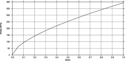
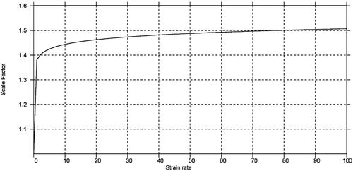
The strain stress data in Figure 12 is adapted to cater for strain rate effects using the scale factor function in Figure 13.

Figure 13. Strain rate effects.

Based on the above specifications 12 baseline FE models were created (one for each cross-section defined in Table 5.

With the numerical model setup complete the focus will now turn to the optimisation setup.

3.4. Optimisation methodology

Although preferable, the employment of direct optimisation techniques was deemed infeasible due to the complexity of the numerical analysis combined with the anticipated number of numerical experiments (FEA runs) required to complete the case study; see Tables 6 and 7 for design variables and constraints. Instead, a Reduced Order Model (ROM) based approach was adopted as defined in the overall flowchart illustrated in Figure 14.

Figure 14. Optimisation study flowchart.

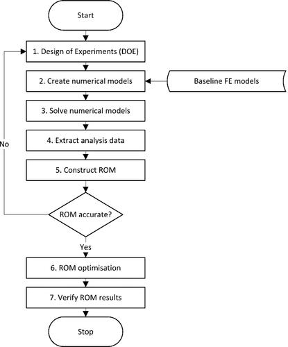
The methodology, Figure 14, was implemented with a combination of user scripts, LS-DYNA explicit FE solver and the ODYSSEE platform for ROM and optimisation inspired by [23]. The process in Figure 14 will be completed once for each of the 12 cross-sections in Table 5 within each of the 6 optimisation studies A-F (Table 7); the same data can be used for _LLM, _IR_40 and _IR_40.

The individual steps of the flowchart in Figure 14 are further described below.

• Step 1: Design of Experiments (DOE) was used to define the numerical experiments, i.e. the variation of optimisation design variables (Table 7).The number of design variables ranges between 1-4 thickness variables Ti and/or 2 FG-SV variables (YZA and YZB). For example, the SQ cross-section in study A will have 1 design variable, whereas the BMCT cross section in study E will have 6. All studies with FG-SV only, i.e. C, D, I and J will have 2 design variables regardless of the cross-section. Hence, the number of design variables ranges between 1-6 and the individual parameter intervals listed in Table 7. As with any DOE study the sampling method is very important to create appropriately accurate ROMs without excessive computational efforts. Factorial DOEs provide robust information gathering capabilities but are often computationally expensive as they require more sampling points than are truly necessary for accurate predictions particularly for highly non-linear systems as the ones considered in this paper. Space filling designs such as (Optimal) Latin Hypercube utilise evenly distributed samples [24] minimizing the computational expense whilst maximizing the potential learning gained from each simulation. Space-filling designs therefore offer high accuracy with reduced sampling points and provide a good starting point to construct the ROMs of the subsequent study. Furthermore, sampling methods such as full-factorial design generally provide focus on the design space boundaries with less emphasis on the centre of the design domain. Consequently, an Optimal Latin HyperCube sampling method requiring 20 numerical experiments for each cross-section, regardless of the number of design variables was initially defined. The total number of FE models for each optimisation study thereby becomes 240 (20 experiments × 12 cross-sections). With 6 optimisation studies (A-F, Table 6) the total number of FE models in the case study of this paper becomes 1,440 (240 experiments × 6 studies). Note that the same model can be used for _IR and the _LLM studies as the BSLM constraints are not applied until the (ROM based) optimisation i.e. step 6, Figure 14.

• Steps 2–3: These steps were completed based on the definition of numerical experiments in step 1. Through scripting and utilising the FE baseline models from section 3.3 all 1,440 models were created and solved using an LS-DYNA Explicit solver in a High Performance Computing (HPC) environment.

• Step 4: Scripting was also used to extract the data required to create the ROM models in step 5, based on the 1,440 FE models. The acceleration, SEA and BSLM were extracted as defined in equations (1), (2) and (3) respectively.

• Step 5: The ODYSSEE suite was used to create the ROM models; the first task is to determine appropriate ROM methods for each of the 3 parameters (SEA, acceleration and BSLM) that govern the subsequent optimisation. This was completed for each of the 12 cross-sections (Table 5) across all 6 optimisation studies (Table 7), i.e. a total of (3 × 12 × 6) 216 methods had to be determined. Using the LUNAR module within the ODYSSEE suite the available methods can broadly be divided into direct interpolation, decomposition-reduction-reconstruction and clustering methods. Within each method a number of solver algorithms such as Kriging, Radial Basis Functions (RBF) and Proper Orthogonal Decomposition (POD) exist. Within each solver algorithm a number of further refinement options such as selecting basis functions also exist [25]. As this methodology was completed 216 times the following explanation demonstrates one parameter only; namely the acceleration of the BMCT cross-sections in optimisation study A. Remembering that 20 numerical experiments (FE models) per cross-section per optimisation study were completed in steps 1-4, the results from 19 of those are used as input data for the ROM as illustrated in Figure 15, whilst the results of the 20^th model were utilised to verify the accuracy of the ROM.

  Figure 15. Study A, BMCT cross-section, acceleration curves.

  

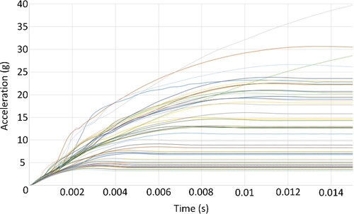
The 19 curves illustrated in Figure 15 enables LUNAR to deduce the links between Ti values and acceleration response by selecting an appropriate ROM method. Subsequently, the Ti values for the 20^th FE model can be to verify the LUNAR prediction thus assessing the accuracy of the individual ROM model. The LUNAR prediction and the FE curve for this particular case are illustrated in Figure 16.

Figure 16. LUNAR prediction vs. numerical analysis result.

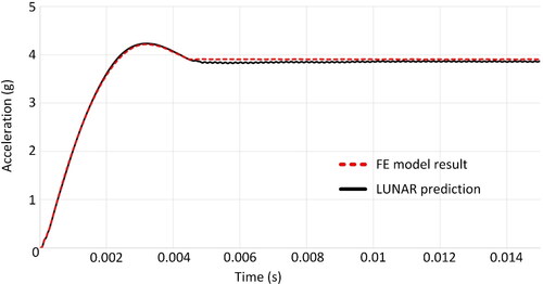
As indicated in Figure 16 the LUNAR predictions include the time history of the individual parameter, enabling a more comprehensive ROM and optimisation as opposed to extracting singular values. Nevertheless, for this benchmarking study the emphasis will be on the maximum (peak) values. In order to evaluate the accuracy of the metamodels a simple ratio comparing the maximum value of the Lunar prediction (Lun_max) to that of the numerical (FE) analysis (FE_max) as defined in equation 4(4) $$\text{ROM}\mathrm{ }\text{accuracy}=\frac{{\mathit{Lun}}_{\mathit{max}}}{{FE}_{\mathit{max}}}$$(4) is introduced. (4) $$\text{ROM}\mathrm{ }\text{accuracy}=\frac{{\mathit{Lun}}_{\mathit{max}}}{{FE}_{\mathit{max}}}$$(4)

Using equation 4(4) $$\text{ROM}\mathrm{ }\text{accuracy}=\frac{{\mathit{Lun}}_{\mathit{max}}}{{FE}_{\mathit{max}}}$$(4) all possible Lunar ROM options were explored to determine the most accurate method to represent each of the 216 ‘signals’ (SEA, acceleration and BSLM × 12 cross-sections, Table 5, × 6 studies, Table 7). As it is infeasible to list the accuracy of all 216 ROM in this paper the ratios (listed in percentage) are summarised in Table 11 as a function of IEAD.

Table 11. Meta-model accuracy by cross-section.

IEAD	SEA			Acceleration			BSLM
	Average	Min	Max	Average	Min	Max	Average	Min	Max
BMCT	101%	95%	106%	98%	95%	102%	104%	87%	106%
CCSPL	102%	97%	111%	102%	98%	112%	98%	88%	107%
Dodecagon	98%	93%	102%	102%	95%	109%	99%	95%	103%
Hexa_0	101%	94%	108%	97%	86%	103%	97%	89%	102%
Hexa_3	101%	99%	104%	100%	98%	101%	99%	98%	100%
Hexa_6	100%	96%	106%	100%	98%	102%	100%	95%	106%
Octa_0	101%	97%	106%	98%	95%	101%	98%	97%	102%
Octa_4	102%	99%	107%	100%	96%	104%	96%	89%	100%
Octa_8	102%	100%	109%	100%	95%	110%	99%	94%	102%
RS	102%	95%	106%	100%	96%	103%	100%	96%	106%
SQ9	101%	99%	106%	99%	98%	100%	95%	64%	104%
SQ	99%	90%	109%	99%	97%	101%	97%	91%	100%

Based on equation 4(4) $$\text{ROM}\mathrm{ }\text{accuracy}=\frac{{\mathit{Lun}}_{\mathit{max}}}{{FE}_{\mathit{max}}}$$(4) , a value below 100% in Table 11 indicates that the ROM predictions are conservative relative to the FE model, whereas values in excess of 100% indicates a liberal prediction. In general, Table 11 shows an average accuracy close to 100% within a ± 10% interval. The greatest variations are found in the BSLM predictions, the reason for this is that these signals have peaks with significant fluctuations in the first 2-3ms of the impact. Although filtering of the signals could potentially reduce this issue it was determined that the values are not numerical noise and should therefore remain unfiltered. Irrespective of these fluctuations Table 11 reveals that the average accuracy is good; the largest fluctuation is found with the minimum value of 64% for SQ9, meaning that the ROM predictions are conservative in this particular instance. At this stage a study into further increasing the ROM accuracy was completed. Based on the SQ9 cross-section and using the design variables of study A, the number of numerical experiments was doubled from 20 to 40. Subsequently 39 sets of data were used as input into LUNAR with the remaining result used for the comparison as illustrated in Figure 16. The study found only a marginal increase in accuracy of approximately 0.8% in this particular case, consequently it was decided not to increase the number of DOE experiments or sampling type across the entire study.

In conclusion, Table 11 shows that the meta-model accuracies are acceptable and do not ‘favour’ or ‘punish’ any specific IEAD with the minor exception of the aforementioned SQ9 BSLM value. The meta-model accuracy as a function of study (A-F, Table 7) was also completed, this also demonstrated that there was no noteworthy difference of ROM accuracy across the different optimisation studies thus verifying that the Optimal Latin Hypercube sampling was effective for the optimisation studies in this paper.

Step 6-7: Based on the ROM created in step 6 and the parameters defined in Tables 6, 7 and 8 the optimisation studies can now be completed. The ROM based optimisation was completed using Sequential Quadratic Programming (SQP) (LLM and IR_40 studies) and the Downhill Simplex Algorithm (IR). The results including verification of results (step 7) will be discussed in the next section.

4. Results and discussion

In this section the results of individual studies will be discussed before comparison between studies are done and overall conclusions drawn. In order to directly compare the structural performance potential of each of the 12 IEADs in an unbiased, yet concise way the results in all subsequent graphs have been normalised with respect to the benchmark square section (SQ Table 5). Please note that all optimisation results presented in this section has been verified through numerical (FE analysis), step 7 Figure 9. This was done using equation 4(4) $$\text{ROM}\mathrm{ }\text{accuracy}=\frac{{\mathit{Lun}}_{\mathit{max}}}{{FE}_{\mathit{max}}}$$(4) with the FE model parameters (Ti, YZA and YZB) defined by the results of the ROM optimisation. The results showed no discernible differences from the data in Table 11 and has therefore been omitted from the paper for conciseness.

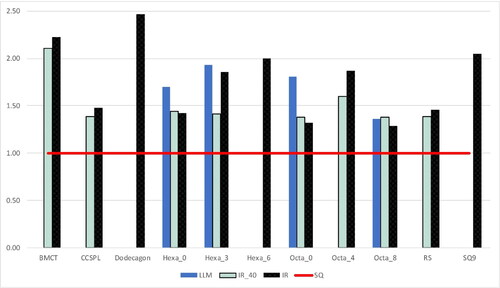
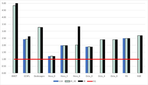
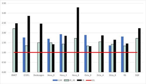
Study A

In study A the specimen length is 200 mm, the impact speed is 2.78 m/s and the only design variables are gauge thickness values (Ti, Table 5). Figure 17 shows the normalised SEA values for each IEAD based on the LLM, IR_40 and IR optimisation results. Note that where a graph is missing, such as the LLM results for BMCT, it indicates that no solution satisfying all constraints were found. The specific details of these have been omitted from the paper for conciseness.

Figure 17. Study A normalised SEA results.

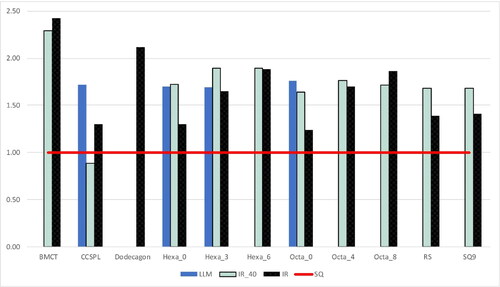
Figure 17 shows that for nearly all instances the IEADs perform better than the SQ in terms of SEA. Note however that only 4 IEADs (CCSPL, Hexa0_0, Hexa_3 and Octa_0) where able to satisfy the LLM constraints (in addition to SQ). Results show that the BSLM constraint was always violated and the acceleration constraint was violated in only one instance where there was no viable LLM result. The acceleration violation is indicated in Figure 17 where there is no result for the IR_40 optimisation. Figure 17 also shows significant variation (across optimisation studies) in the performance of individual IEAD relative to the SQ benchmark. An obvious example is CCSPL where the SEA is higher for the LLM and IR optimisation but lower for the IR_40 relative to the SQ benchmark. Figure 18 shows the results from the unconstrained (IR) optimisation study.

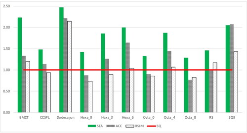
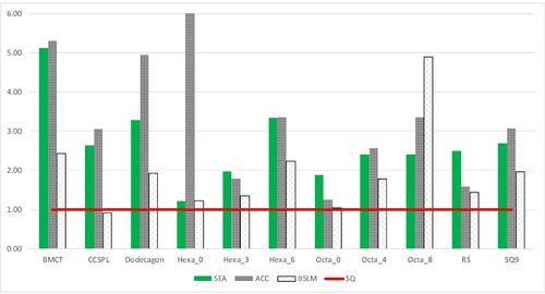
Figure 18. Study A IR results.

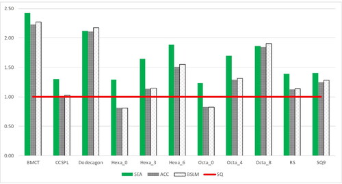
In Figure 18 ‘excellent’ performance would consist of an SEA value significantly higher combined with acceleration and BSLM values lower than the SQ benchmark. This is for example the case with Hexa_0 and Octa_0. BMCT and Dodecagon provide significantly higher SEA values but with almost equal increases in acceleration and BSLM magnitudes effectively making these scalars of the SQ benchmark as opposed to significantly increased overall performance. As discussed, the acceleration levels could potentially be reduced through the introduction of crash initiators; this is however not the case for BSLM. Finally, the significantly increased complexity of the cross-sections of e.g. the BMCT compared to the simplicity of the SQ is of course also a consideration in practical applications.

Study B

In study B the specimen length is 400 mm, the impact speed is 15 m/s and the only design variables are gauge thickness values (Ti, Table 5). Figure 19 shows the normalised SEA values for each IEAD based on the LLM, IR_40 and IR optimisation results.

Figure 19. Study B normalised SEA results.

The overall trends from Figure 17 are also evident in Figure 19 namely that the SEA of all IEAD tested exceed that of the SQ. As in Study A only 4 (in addition to SQ) were able to meet the LLM constraints; three of which are identical (Hexa_0, Hexa_3 and Octa_0). For the remaining ones the BSLM constraint was always violated with three IEAD also violating the acceleration constraint. The indicated improved performance of CCSPL has drastically reduced in comparison to Study A.

Figure 20 displays interesting trends, namely that all IEADs investigated improve overall performance relative to SQ. This is particularly evident for Hexa_0 where the SEA is increased, but both acceleration and BSLM values are reduced. Hexa_6 provides the largest increase in SEA with only a marginal increase in BSLM. The Dodecagon provides the largest overall increase in SEA but equally provides the largest increases of acceleration and BSLM; i.e. almost a linear scalar of all parameters as identified in Study A.

Figure 20. Study B IR results.

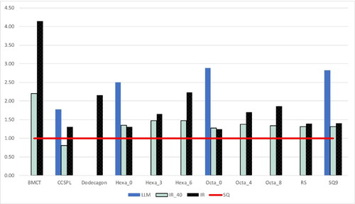
Study C

In study C the Ti values are all set to unity, the specimen length is 200 mm, the impact speed is 2.78 m/s. The aim is to explore the isolated effects of FG-SV (Figures 2 and 11), and so the only design variables are the morph variables YZA and YZB. Figure 21 shows the normalised SEA values for each IEAD based on the LLM, IR_40 and IR optimisation results.

Figure 21. Study C normalised SEA results.

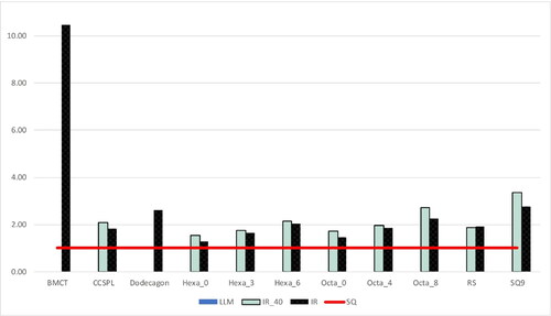
Figure 21 also shows an SEA increase across all IEADs. However, in this case none (including SQ) were able to meet the LLM constraints indicating that functional grading (FG-SV) is a less influential design variable compared to gauge thickness. In line with studies A and B the dominating constraint is BSLM. The IR results, Figure 22, show very high SEA increases, but the BSLM limit is also drastically increased.

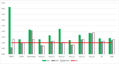
Figure 22. Study C IR results.

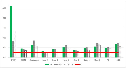
Consistent with previous studies Hexa_0 is seeming the best overall solution due to an increase of SEA without any increase of acceleration or BSLM. The results also indicate that in some instances, e.g. Octa_8, the increase in SEA is less than the increase of acceleration and BSLM. Although this is also the case for individual IEADs in studies A and B it is more prevalent in study C (Figure 22). It should also be noted that the SQ9 BSLM magnitude in Figure 22 is likely to be conservative due to the lower ROM correlation as discussed in the previous section. The FE validation found the BSLM value to be approximately 20% higher than indicated in Figure 22.

Study D

In study D the Ti values are all set to unity, the specimen length is 400 mm, the impact speed is 15 m/s. Figure 23 shows the normalised SEA values for each IEAD based on the LLM, IR_40 and IR optimisation results. The results are generally consistent with the trends of Study C; however there is a significant increase in the number of IEADs meeting the LLM study constraints.

Figure 23. Study D normalised SEA results.

The IR results in Figure 24 show that Octa_0 provides the most increase in SEA with no increase in BSLM. BMCT once again provides the largest increase in SEA and although the BSLM is not increased equally it remains 2.3 times higher than the SQ benchmark.

Figure 24. Study D IR results.

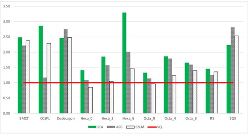
Study E

Study E explores the combined effects of thickness (Ti) and functional grading (FG-SV). In this study the specimen length is 200 mm and the impact speed is 2.78 m/s. Figure 25 shows the normalised SEA values for each IEAD based on the LLM, IR_40 and IR optimisation results. The results follow the general trends of Studies A and C wherein SEA is increased for almost every scenario with the exception of CCPSL in the IR_40 optimisation. Also note that the BMCT did not meet the LLM constraints as is the case of the Dodecagon which furthermore did not meet the IR_40 constraint. Of particular interest is CCSPL, Hexa_0, Octa_0 and SQ9 which all provide significant increase in SEA whilst meeting the LLM constraints compared to the SQ benchmark.

Figure 25. Study E normalised SEA results.

The IR results, Figure 26, are particularly encouraging for the Hexa ‘family’ wherein all demonstrate a noteworthy increase of SEA with a reduction of BSLM and acceleration (Hexa_0) or a marginal increase (Hexa_3 and 6). Similar comments can be made about Octa_0, RS and CCSPL. The largest SEA increase by a factor of approximately 4.1 is however from the BMCT. This combined optimisation (Ti and FG-SV) does indicate a much better ratio of SEA to BSLM increase when compared to the separate investigations in studies A (Figure 18) and C (Figure 22).

Figure 26. Study E IR results.

Study F

Study F is analogue to E but utilises a specimen length of 400 mm and an impact speed of 15 m/s. Figure 27 shows the normalised SEA values for each IEAD based on the LLM, IR_40 and IR optimisation results.

Figure 27. Study F normalised SEA results.

The results follow the general trends of Studies B and D wherein SEA is increased across all IEADs. Also note that the BMCT, Dodecagon, Hexa_6, Octa_4 and SQ9 did not meet the LLM constraints. The remaining IEADs provide significant increase in SEA whilst meeting the LLM constraints compared to the SQ benchmark. The results of the IR optimisation, Figure 28, show significant variations of trends when compared to study E (Figure 26). In this case the BMCT does provide an increase in SEA, but the BSLM is increased almost equally. Hexa_0 retains the trend of increased SEA with a decrease in BSLM as does Octa_0. The highest SEA increase comes from Hexa_6 which also shows an increase in BSLM of approximately 1.5 whereas Hexa_3 represents the highest increase in SEA with only a marginal increase of BSLM.

Figure 28. Study F IR results.

General trends

Based on the results from studies A-F overall trends covering all IEADs, multi-cell and multi-corner cross-sections as well as the influence of FG-SV can now be explored benchmarked to the SQ cross-section. Table 12 shows the average increase of SEA, acceleration and BSLM magnitudes as a function of design variables, cross-section type and impact velocity/specimen length based on the IR optimisation studies. As previously defined the CCSPL, Octa_0 and Hexa_0 represent multi-corner cross-sections whilst the remaining cross-sections are multi-cell.

Table 12. Overall results based on IR optimisation studies.

Design variables	Cross-sections	Data source study	Average increase
			2.78 m/s			15 m/s
			SEA	ACC	BSLM	SEA	ACC	BSLM
Thickness (Ti)	All IEADs	A & B	66%	38%	41%	77%	33%	12%
	multi-cell only		80%	56%	60%	90%	47%	22%
	multi-corner only		28%	−11%	−11%	41%	−3%	−16%
FG-SV (YZ-A & YZ-B)	All IEADs	C & D	174%	130%	107%	168%	230%	93%
	multi-cell only		219%	165%	139%	196%	225%	125%
	multi-corner only		53%	36%	22%	91%	246%	7%
Thickness and FG-SV	All IEADs	E & F	85%	18%	19%	108%	77%	63%
	multi-cell only		107%	30%	31%	116%	100%	73%
	multi-corner only		28%	−12%	−14%	87%	13%	37%

Table 12 reveals significant fluctuations in the improvement of SEA relative to the SQ benchmark, the largest of which can be found in connection with the FG-SV. It is however also evident that the largest increases of acceleration and BSLM magnitudes also occurs in this connection highlighting the fact that the increase in SEA may also lead to drawbacks. In general Table 12 indicates that the largest average SEA increase relates to the multi-cell cross-sections, but this generally also comes with an increase of acceleration and BSLM. In contrast the general trend of the multi-corner cross-sections are more moderate SEA increase but with reductions of acceleration and BSLM magnitudes relative to the multi-cell cross-sections. An example of this is the 2.78 m/s impact with the thickness only design variables; in this case the multi-cell cross-sections have an average SEA increase of 80% but also a 56% acceleration and 60% BSLM magnitude increase. The corresponding multi-corner studies show a more moderate 28% SEA increase this is however accompanied with 11% decreases of acceleration and BSLM, i.e. 67% and 71% less compared to the multi-cell.

5. Conclusion

This paper provides a first unbiased benchmark study covering a range of specific recently proposed IEADs focusing on automotive crash structure applications. The accuracy of the results obtained via ROM are verified via a series of separate numerical (FE) models. The optimisation studies show that all IEADs considered do indeed carry potential for increased SEA relative to the benchmark square (SQ) cross-section; this does however often come at a cost of increased acceleration and/or BSLM magnitudes making the ‘real-world’ benefits less clear. This paper does not identify a single cross-section or even type of cross-section (multi-cell or multi-angle) with a consistent best potential because, as expected, this significantly depends on the actual application, e.g. crush can or longitudinal. Furthermore, the inclusion of geometric details such as crash initiators can potentially significantly reduce peak acceleration levels. The results show that functional grading through shape-variation (FG-SV) provides the largest relative increase of SEA, but also provide the largest increase in acceleration and BSLM magnitudes. Multi-cell structures provide the best SEA increase on average, but do also lead to increases of acceleration and BSLM. Multi-angle cross-sections provide more moderate increases of SEA, but generally lead to acceleration and BSLM reductions. The studies in this paper were completed on a component basis and although the authors believe that the benchmarks of this paper are generally representative of system level potential (i.e. a combined crush can and longitudinal structure) this should be subsequently explored to further evaluate the potential of the IEADS for industrial applications. The results of this paper should therefore serve as indicators of potential for specific applications and further research into the development of effective crash-structures for future vehicle applications.

Acknowledgements

The authors would like to thank Sandrine Le Corre and Dorian Salin of CADLM for providing software support during the methodology implementation.

Disclosure statement

The authors have no potential competing interests to report.

References

- Baroutaji A, Sajjia M, Olabi AG. On the crashworthiness performance of thin-walled energy absorbers: Recent advances and future developments. Thin-Walled Struct. 2017;118:137–163.
- Chang Q, Yang S. Crashworthiness and lightweight optimisation of thin-walled conical tubes subjected to an oblique impact. Int J Crashworthiness. 2014;19(4):334–351.
- Asanjarani A, Dibajian SH, Mahdian A. Multi-objective crashworthiness optimization of tapered thin-walled square tubes with indentations. Thin-Walled Struct. 2017;116:26–36.
- Guangyao L, Fengxiang X, Sun SG, et al. A comparative study on thin-walled structures with functionally graded thickness (FGT) and tapered tubes withstanding oblique impact loading. Int J Impact Eng. 2015;77:68–83.
- Sun G, Pang T, Xu C, et al. Energy absorption mechanics for variable thickness thin-walled structures. Thin-Walled Struct. 2017;118:214–228.
- Zhang X, Wen Z, Zhang H. Axial crushing and optimal design of square tubes with graded thickness. Thin-Walled Struct. 2014;84:263–274.
- Chen Y, Bai Z, Zhang L, et al. Crashworthiness analysis of octagonal multi-cell tube with functionally graded thickness under multiple loading angles. Thin-Walled Struct. 2017;110:133–139.
- An X, Gao Y, Fang J, et al. Crashworthiness design for foam-filled thin-walled structures with functionally lateral graded thickness sheets. Thin-Walled Struct. 2015;91:63–71.
- Zheng G, Pang T, Sun G, et al. Theoretical, numerical, and experimental study on laterally variable thickness (LVT) multi-cell tubes for crashworthiness. Int J Mech Sci. 2016;118:283–297.
- Fang J, Gao Y, An X, et al. Design of transversely-graded foam and wall thickness structures for crashworthiness criteria. Compos Part B. 2016;92:338–349.
- Ebrahimi S, Vahdatazad N, Liaghat G. Crashworthiness efficiency optimisation for two-directional functionally graded foam-filled tubes under axial crushing impacts. Int J Crashworthiness. 2017;22(3):307–321.
- Zhang Y, Ge P, Lu M, et al. Crashworthiness study for multi-cell composite filling structures. Int J Crashworthiness. 2018;23(1):32–46.
- Gao Q, Wang L, Wang Y, et al. Crushing analysis and multiobjective crashworthiness optimization of foam-filled ellipse tubes under oblique impact loading. Thin-Walled Struct. 2016;100:105–112.
- Yin H, Wen G, Liu Z, et al. Crashworthiness optimization design for foam-filled multi-cell thin-walled structures. Thin-Walled Struct. 2014;75:8–17.
- Zhang Y, Sun G, Xu X, et al. Multiobjective crashworthiness optimization of hollow and conical tubes for multiple load cases. Thin-Walled Struct. 2014;82:331–342.
- Chen S, Yu H, Fang J. A novel multi-cell tubal structure with circular corners for crashworthiness. Thin-Walled Struct. 2018;122:329–343.
- Qiu N, Gao Y, Fang J, et al. Theoretical prediction and optimization of multi-cell hexagonal tubes under axial crashing. Thin-Walled Struct. 2016;102:111–121.
- Li J, Gao G, Zou X, et al. Crushing analysis and multiobjective crashworthiness optimization of bitubular polygonal tubes with internal walls. J Cent South Univ. 2016;23(11):3040–3050.
- Sun G, Pang T, Fang J, et al. Parameterization of criss-cross configurations for multiobjective crashworthiness optimization. Int J Mech Sci. 2017;124-125:145–167.
- Zhang L, Bai Z, Bai F. Crashworthiness design for bio-inspired multi-cell tubes with quadrilateral, hexagonal and octagonal sections. Thin-Walled Struct. 2018;122:42–51.
- Bastien C. 2014. “The prediction of kinematics and injuries of unbelted occupants under autonomous emergency braking.” Available from: <https://www.researchgate.net/publication/265335888_The_Prediction_Of_Kinematics_And_Injury_Criteria_Of_Unbelted_Occupants_Under_Autonomous_Emergency_Braking. > (last accessed 27/04/2021).
- SAE International. “ Instrumentation for impact test – part 1- electronic instrumentation.” Available from: <https://www.sae.org/standards/content/j211/1_201403/. > (last accessed 23/03/2021).
- Kayvantash K, Thiam A, Ryckelynck D, Chaabane SB, Touzeau J, Ravier P. 2015. “Model order reduction techniques for real-time parametric crash and safety simulations.” Available from: <https://www.dynalook.com/conferences/10th-european-ls-dyna-conference/3%20Process%20IX%20-%20Cutting-Model%20Reduction/04-Kayvantash-CADLM-P.pdf. > (last accessed 22/04/2021).
- Park J. Optimal latin-hypercube designs for computer experiments. J Stat Plan Infer. 1994;39(1):95–111.
- Revolutions In Simulation 2021. “Model order reduction techniques for real-time parametric crash and safety simulations,” Available from <https://revolutioninsimulation.org/wp-content/uploads/2021/02/ROM_Kambiz_Kayvantash_CAHRS_paper.pdf> (last accessed 01/05/2021).