Conditional space evaluation of progress variable definitions for Cambridge/Sandia swirl flames

Abstract

Data from all spatial locations of nine turbulent flames in the Cambridge/Sandia swirl database are combined to study how the choice of scalar variables in conditional moment closure (CMC) type approaches affect the conditional spatial fluctuations of reactive scalars. In order to investigate the influence of swirl and stratification, two additional data-sets have been constructed. Principal component analysis (PCA) is applied to help identify the number of scalar variables and the most appropriate choices to describe the composition space. Two PCA scaling methods have been adopted, namely Pareto and Auto-scaling. Regardless of the data-set investigated and the scaling method used, the results suggest that a single principal component correlated with temperature accounted for the largest variance. For the first moment hypothesis, four progress variable, c, definitions identified by PCA are selected as conditioning variables to investigate the conditional fluctuations and normalised RMS of various species and temperature from all three databases at all axial locations. The results indicate that two control variables based on mixture fraction, Z, and progress variable significantly reduce the conditional fluctuations of scalars compared to a single variable. The selection of progress variables had minimal effects on the RMS of conditional fluctuations for all tested conditions, although a slight reduction of conditional fluctuations was found for the temperature-based progress variable, which can potentially help the further extension of CMC-based models in different flame configurations. The present study also shows that using Z and c (regardless of its definition) as two conditioning scalars enables the detachment of the thermo-chemical state from space, swirl and stratification effects. This suggests that adopting a doubly conditioned source term estimation (DCSE) approach might successfully predict the considered set of flames, assuming that ensembles are divided along the axial direction.

Keywords:

• numerical simulation
• Turbulent combustion
• principal component analysis
• conditional moment method

1. Introduction

For simulations that are not fully resolved, closure of the chemical source term is needed. Various methodologies have been developed (e.g. the flamelet model [1], or the conditional moment closure approach [2]) to build functional filtered chemistry models that can close the highly non-linear source term. Although based on different assumptions, the accuracy of these models relies on (i) an adequate description of the composition space, which seeks to relate the different scalar variables in the thermo-chemical scalars' vector, and (ii) an adequate description of the statistical distribution of these variables in the form of a joint probability density function (PDF).

Among different models and studies, local mixture, the degree of progression of the chemical reactions, strain rate, total enthalpy, and residence time are properties that have been found to be closely related to the chemical rates in a reactive flow field. For non-premixed flames, the mixture fraction, Z, is usually retained as the main controlling variable to describe the turbulent mixing effects [3]. For premixed flames, the progress variable, c, is often selected as the primary scalar to describe the rate of progression from the unburnt to burnt state [4]. It has been shown that the fluctuations found in the species mass fractions and temperature are often correlated in non-premixed flames with the fluctuations of Z and with the fluctuations of c in premixed flames. However, a single scalar variable able to accurately describe the structure of partially-premixed flames and capture regions with high probabilities of local extinction and re-ignition has not yet been found [5,6]. This has led to different combinations of scalar variables, where often the mixture fraction and the progress variable are simultaneously considered [7]. The inclusion of two different mixture fractions as control variables was also proposed to capture the main properties of moderate and intense low oxygen dilution (MILD) combustion for jet-in-hot-coflow (JHC) burners [8–11]. While mixture fractions are generally incorporated using Bilger's definition [12], various definitions of the progress variable have been used for different approaches.

For laminar flamelet approaches, progress variables are often chosen as the primary controlling variables to construct a reduced dimension composition space. The temperature and the mass fraction of a major combustion product (e.g. H${}_2$O or CO${}_2$) have been widely used to define c for flamelet models. While suitable for many flames, using a single product mass fraction for larger hydrocarbons may fail to represent the progress of the chemical reactions. Therefore, more species mass fractions in the form of linear combinations are often incorporated to track the reaction progress in the flow and capture different stages of combustion [13,14]. Sun et al. [15] have investigated the modelling capabilities of the unsteady flamelet/progress variable (UFPV) model in predicting the ECN Spray A cases. The progress variable was defined using a combination of major and intermediate species to obtain results across all downstream locations of the jet. While progress variables incorporating more than a single species mass fraction are effectively better performing, two challenges are worth mentioning, of which (i) the diffusivity of the selected scalars needs to be accounted for in the progress variable transport equation, and (ii) the addition of intermediate species is often in conflict with the monotonicity of c. Studies have tackled the injection of the progress variable by computing weight coefficients using various automated optimisation techniques, e.g. the well-known $\frac{\mathrm{\partial }c}{\mathrm{\partial }\kappa }>0$ criterion, where κ often denotes a time or a spatial coordinate [16–18]. However, most progress variable definitions found in the literature are based on user expertise where the chosen definition can significantly influence the numerical predictions, particularly for fuel-rich/heavy-fuel mixtures [19]. Recently, Gupta et al. [20] studied different progress variable definitions for tabulated chemistry through the analysis of premixed methane-air (CH${}_4$/Air) laminar flames. Compared with detailed chemistry, flamelet generated manifold (FGM) results using different species mass fraction-based progress variable definitions were shown to give different mass burning rates. Lipatnikov & Sabelnikov [21] also examined the effect of five different progress variable definitions on the flamelet approach predictions of the mean density and the mean mole fractions of various species using Direct Numerical Simulation (DNS) data of a premixed hydrogen-air flame. A complementary study was carried out using DNS data of lean hydrogen-air turbulent premixed flames operating under various Karlovitz numbers [22]. Similar findings were obtained, suggesting that the definition of c in flamelet-based models indeed affects the physical modelling while simultaneously impacting numerical errors.

For conditional moment closure (CMC) models, filtered chemistry is modelled through the separation of model elements which give descriptions for the moments of reactive parameters and model of the distribution function. CMC-based approaches are centred around the hypothesis that fluctuations in reactive scalars are closely correlated with the fluctuations around values of conditioning variables (e.g. mixture fraction and progress variable) [23,24]. Originated from CMC, conditional source term estimation (CSE) avoids solving conditionally-averaged transport equations by inversion of the integral functions [25]. In a recent work on the methane-air non-premixed piloted Sandia flames, CSE was found to provide a more accurate solution while being less time-consuming compared to CMC [26]. CSE models have also been used to simulate large hydrocarbon and spray flames. While using CSE-based approaches with a single conditioning variable has been found suitable for non-premixed and premixed flames [7,27–30], for partially-premixed or stratified combustion, one conditioning variable is not sufficient. Subsequently, doubly CSE (DCSE) with mixture fraction and progress variable as conditioning variables have been developed to simulate partially-premixed flames, lifted flames, and spray flames [31,32]. The CSE and DCSE concepts have also been examined in a-priori analysis in DNS for high-pressure conditions [33]. The results highlighted that DCSE and double conditioning are likely to be needed for cases closer to real practical combustion applications. Similar to the flamelet approaches, when choosing the conditioning variables for CMC approaches, the mixture fraction definition from Bilger is well accepted by the community, where the choice of progress variable and particularly its effects on conditional variable fluctuations needs more studies. Recently, Bushe [34] and Mousemi & Bushe [35] examined the conditional moment closure hypothesis over the Sandia/TUD, the Sydney Swirl burner, and Cambridge/Sandia stratified swirl burner databases. Their studies suggested two-condition (mixture fraction and progress variable) conditional averages in the Sandia/TUD do not vary in space nor vary with the Reynolds number, whereas, for Sydney and Cambridge/Sandia swirl burners, a third conditional variable (total enthalpy) might be needed to further reduce the spatial gradients of conditional averages attributed to the heat transfer. For these studies, progress variables based on temperature and mass fraction of CO${}_2$ were used. Perhaps more interestingly, the a-priori studies on single-step high-pressure DNS data from Devaud et al. [33] and Bushe et al. [36] using CO${}_2$ and temperature-based progress variables suggested the success of DCSE does not depend on a particular choice of the second conditioning variable which significantly increased the capabilities of CSE models. However, further extension of these two studies on the effect of progress variable selections is not possible due to the single-step chemistry nature of the DNS data.

Consequently, two questions around control variables in the context of CMC-based models are worthy of note here – the questions central to this paper:

1. What is the minimum number of scalar variables needed to adequately characterise conditional space for certain flames?

2. Which scalar variables represent the best choices for this, and how do they influence the predictions, in particular for the definition of the progress variable?

Depending on the studied case, Bushe et al. [34] also pointed out that the selection and number of control variables must be carefully undertaken to adequately address the effects of turbulence and chemistry. Additionally, the modelling of the joint-PDF gives a substantial challenge to the turbulent combustion modelling community as its shape strongly depends on the selected scalar variables. The validity of the statistical independence assumption used for modelling the presumed joint-PDF was shown to be erroneous, as correlations between conditional variables are important [36].

The present work is motivated by the study of three different groups: Sutherland & Parente's work on principal component analysis-based models [37], Bushe's study on spatial gradients of conditional averages [34], and Gupta et al.'s analysis on the impact of the progress variable definition on flamelet generated manifolds [20]. We investigate the two questions posed above with a particular focus on the effect of progress variable selection on the conditional fluctuations obtained with one-condition conditional averages and doubly conditional averages of the Cambridge/Sandia swirl burner data-set. We will first introduce the properties and working conditions of the burner and the methodology employed for determining the appropriate progress variable definitions. The chosen progress variable definitions are then used to study conditional fluctuations where all one-point, one-time measurements are included. The results are discussed, and physical insights are provided based on the observations.

2. Methodology

2.1. Experimental setup

Experimental measurements of premixed and stratified CH${}_4$/Air flames from the Cambridge/Sandia swirl burner (referred to as SwB) are used in this study. Multiscalar data of nine turbulent flames are examined under: (i) various ratios of stratification, and (ii) various swirl intensity conditions, depicted in Table 1.

Table 1. Operating conditions for Cambridge/Sandia swirl burner. ${\varphi }_i$ and ${\varphi }_o$ denote equivalence ratio of the flow in the inner and outer annuli, respectively. In all cases ${\varphi }_g=0.75$, $U_i=8.31$ m/s, $U_o=18.7$ m/s and $U_{co-flow}=0.4$ m/s. Conditions highlighted in bold font denote flames under swirling flows.

Flame	Swirl ratio	Stratification factor	${\varphi }_i$	${\varphi }_o$
SwB1	0	1	0.75	0.75
SwB2	0.25	1	0.75	0.75
SwB3	0.33	1	0.75	0.75
SwB5	0	2	1	0.5
SwB6	0.25	2	1	0.5
SwB7	0.33	2	1	0.5
SwB9	0	3	1.125	0.375
SwB10	0.25	3	1.125	0.375
SwB11	0.33	3	1.125	0.375

The burner, shown schematically in Figure 1, features a large co-flow of pure filtered air preventing ambient air from entering the reaction zone, and two concentric outer (subscript o) and inner (subscript i) annuli supplying the fuel/air mixture. The annuli's velocities were chosen to maximise the Reynolds numbers in the flows with Re${}_i=$ 5,960 and Re${}_o=$ 11,500. A variable degree of swirl allows the burner to mimic the flow conditions found in many practical systems. The swirl assists flame stabilisation allowing more extreme stratified conditions to be investigated than would otherwise be possible. The stratification factor is defined by the ratio of the equivalence ratio in the inner and outer annuli. The scalar measurements recorded include temperature and the mole fractions of CO${}_2$, CO, H${}_2$, CH${}_4$, N${}_2$, O${}_2$ and H${}_2$O at different axial and radial positions. A minimum of 300 samples were taken at 60 different radial locations per axial position via Rayleigh and Raman scattering to capture temperature and major species, respectively. Further information on the measurement techniques, the experimental setup and the burner's characteristics can be found in [38,39]. The existence of turbulent regions within the flames, operating under premixed and/or stratified mixture conditions, with or without swirl, makes this burner an ideal test case for attempting to answer the two questions central to this paper.

Figure 1. Plan view schematic of the exit geometry in the Cambridge/Sandia swirl burner, showing a plan view and a cross section through the burner axis. The curved-dashed arrows in the plan view indicate the direction of swirling flows in the outer annulus. ${\varphi }_i$ and ${\varphi }_o$ in the cross section denote the equivalence ratio of the flow in the inner and outer annuli, respectively. Adapted from [38]

2.2. Data-processing

Three data-sets have been constructed to investigate the effects of spatial coordinates, swirl flow ratio, and stratification factor on the conditionally-averaged reactive scalars, depicted in Table 2. In the first case, the data collected from all nine flames are grouped together to create a general conditional domain for each of the scalars (SwB$|$all). Here, it is assumed that the conditional averages are independent of spatial coordinate, swirl flow ratio and stratification factor. The second data-set (SwB$|$Hstratified) combines the measurements of three flames exhibiting varying swirl flow ratio intensities with a single high stratification factor to investigate the dependence of conditional averages on swirl. For the third case, data from 3 flames with different stratification factors and a fixed high swirl flow ratio are grouped to investigate the dependence of conditional averages on stratification (SwB$|$Hswirl). Grouping the flames in these three distinct data-sets, each tackling a specific characteristic of the flow, allows the exploration of the most optimal scalar or combination of scalars needed to sufficiently accurately represent the thermo-chemical state under different conditions.

Table 2. Characteristics of the three data-sets used for investigating the behaviour of conditional averages.

Case	Flames	Swirl ratio	Stratification factor	Comments
SwB$|$all	SwB1-11	0–0.33	1–3	All nine flames grouped together
SwB$|$Hstratified	SwB9-11	0–0.33	3	Fixed high stratification
SwB$|$Hswirl	SwB3,7,11	0.33	1–3	Fixed high swirl

The data was first ‘cleaned’ to remove mole fractions displaying negative values associated with experimental uncertainty. All mole fraction measurements were subsequently converted to mass fractions values (note that mass fractions will be used throughout the present work). An extensive analysis of the scalars profiles showed that the measurements of ${\mathrm{Y}}_{\mathrm{H}2}$ are concatenated between the interval $[0,0.0002]$ for all three data-sets. As such, an artificial exclusion for values of H${}_2$ mass fraction above 0.00025 is adopted and carried out to remove potential outliers. The mixture fraction Z was calculated for every instantaneous single-point measurement. The definition of Z proposed by Bilger is used to calculate the mixture fraction of all nine flames, as (1) $\begin{array}{r}Z=\frac{2\frac{Y_{\mathrm{C}}-Y_{\mathrm{C},2}}{M_{\mathrm{C}}}+\frac{1}{2}\frac{Y_{\mathrm{H}}-Y_{\mathrm{H},2}}{M_{\mathrm{H}}}-\frac{Y_{\mathrm{O}}-Y_{\mathrm{O},2}}{M_{\mathrm{O}}}}{2\frac{Y_{\mathrm{C},1}-Y_{\mathrm{C},2}}{M_{\mathrm{C}}}+\frac{1}{2}\frac{Y_{\mathrm{H},1}-Y_{\mathrm{H},2}}{M_{\mathrm{H}}}-\frac{Y_{\mathrm{O},1}-Y_{\mathrm{O},2}}{M_{\mathrm{O}}}}\end{array}$(1) Mixture fractions of zero and unity are respectively assigned to pure air and the richest entry of the flow through all of the cases with an equivalence ratio of 1.125. For the considered sets of flames, the stoichiometric mixture fraction lies at $Z_{\mathrm{s}\mathrm{t}\mathrm{o}\mathrm{i}\mathrm{c}\mathrm{h}}=0.9$, with a lower flammability limit located at Z = 0.575 [40]. To investigate the role of control variables in conditional spaces, four of the most common combustion progress variable c used by the community are considered in this study, defined as (2) $\begin{array}{r}{c}_k=\frac{{\varphi }_k-{\varphi }_{k,min}}{{\varphi }_{k,max}-{\varphi }_{k,min}}\end{array}$(2) where ${\varphi }_1$ denotes the temperature, while ${\varphi }_2$, ${\varphi }_3$ and ${\varphi }_4$ are the mass fractions of ${\mathrm{C}\mathrm{O}}_2$, $\mathrm{C}\mathrm{O}+{\mathrm{C}\mathrm{O}}_2$ and $\mathrm{C}\mathrm{O}+{\mathrm{H}}_2+{\mathrm{H}}_2\mathrm{O}+{\mathrm{C}\mathrm{O}}_2$, respectively (cf. Table 3). The local maximum is determined using a function that returns the upper peak envelopes of the scalar k selected to define c. The envelope is computed using spline interpolation over local maxima separated by 2,500 samples, for which a parametric study was performed to find the optimal number of samples. The local minimum values have been fixed to zero and to 290 K for the species-based progress variables and temperature, respectively.

Table 3. Summary of the four progress variables investigated in this study using Equation (2(2) $\begin{array}{r}{c}_k=\frac{{\varphi }_k-{\varphi }_{k,min}}{{\varphi }_{k,max}-{\varphi }_{k,min}}\end{array}$(2) ).

Label	Scalar(s) ${\varphi }_k$	Mark
$c_1$	Temperature	$◼$
$c_2$	Y${}_{\mathrm{C}\mathrm{O}2}$	$▴$
$c_3$	Y${}_{\mathrm{C}\mathrm{O}2}$ + Y${}_{\mathrm{C}\mathrm{O}}$	$\bullet$
$c_4$	Y${}_{\mathrm{C}\mathrm{O}}$ + Y${}_{\mathrm{H}2}$ + Y${}_{\mathrm{H}2\mathrm{O}}$ + Y${}_{\mathrm{C}\mathrm{O}2}$	♦

A second condition based on mixture fraction and the four progress variables (i.e. $Z,c_k<0$ and $Z,c_k>1$) is applied to take potential outliers from the analysis as these points are considered to be unphysical. After executing all previous steps, each database consists of 5,518,536 point-based measurements for SwB$|$all, 1,887,496 for SwB$|$Hstratified and 1,901,113 for SwB$|$Hswirl.

To examine the conditional space of Cambridge/Sandia flames, the methodology proposed in [34,40] is followed and applied to all three data-sets. The conditional averages are obtained via a discrete process involving binning, dividing each progress variable dimension into 30 bins. This is justified given that more bins increase the possibility of having intervals with an insufficient number of data points which imposes unrealistically small fluctuations around the mean value [40]. Moreover, considering that DCSE will likely be needed for modelling reactive flows relevant to practical combustion systems [33], if more bins are included then more computational time is needed during the inversion process with the matrix of the joint-PDF. This implies that a much larger matrix needs to be inverted compared to previous implementations of CSE in premixed and non-premixed flames. Consequently, the inversion process becomes much more challenging. For the first moment hypothesis, the conditional fluctuations of species mass fractions and temperature around one-condition ($c_1$–$c_4$) conditional average are calculated at each axial location, such that (3) $\begin{array}{r}{f}_{i,k}^{\mathrm{\prime }}=f_i-〈f|\xi =c_k〉\left(x\right)\end{array}$(3) where i denotes a single-point measurement, $f_{i,k}^{\mathrm{\prime }}$ is the fluctuation of either mass fraction or temperature around one-condition ($c_k$), $f_i$ is the point measurement of that reactive scalar and $〈f|\xi 〉\left(x\right)$ is the conditional average of that reactive scalar evaluated by averaging all of the measurements of the chosen data-set at all radial locations together at each downstream distance. Two reasons for investigating how much conditional averages vary in the axial direction are worth mentioning. First, the conditional fluctuations are larger in the axial positions and are spatially independent in the radial direction [34,41]. That was shown to be particularly true for jet flames, suggesting that within a CSE framework, group of localised cells, referred to as an ensemble, should be divided along the axial direction. Second, Mousemi et al. [40] showed for the same burner that the global conditional averages (equivalent to defining a single CSE/DCSE ensemble where all of the reactive control volumes in the domain are included) did not exhibit a particular functional dependence on the flow dynamics and the burner's geometry assuming that three conditioning variables are selected/retained. Suppose that ensembles are split across all axial positions, the number of conditioning scalars needed to accurately represent the chemical state is reduced, where a single control variable could perhaps be sufficient to separate the conditional averages from spatial coordinate, swirl and/or stratification effects. This approach is of particular interest for CMC-based models as it can be seen as a viable alternative to bypass the challenges associated with joint-PDFs defined by a minimum of two scalars.

If the conditional average is a good representation of the local thermo-chemical state, then it is expected that the mean of the conditional fluctuations will be zero. However, the RMS of those fluctuations is clearly not, as shown by Bushe [34] using the Sandia/TUD database and the Sydney swirl burner. Therefore, the square root of the average of the square of conditional fluctuations can be computed, as (4) $\begin{array}{r}{\mathrm{R}\mathrm{M}\mathrm{S}}_{i,k}=\sqrt{〈f_{i,k}^{\mathrm{\prime }2}〉}\end{array}$(4) The proposed RMS is normalised by the maximum value of the considered reactive scalar. This last step is justified in two ways: (i) to compare the different scalars to one another which the relative magnitude should be comparable, and (ii) the data has been filtered to eliminate outliers, suggesting that the maximum measured value is unlikely to be the consequence of a major measurement error.

2.3. Principal component analysis

Over the past decade, low-dimensional manifold representations have been frequently used to mitigate the costs associated with turbulent reacting flows and detailed kinetics [42]. Data-driven analytical tools have seen considerable success in combustion applications for building low-dimensional manifolds while preserving an adequate representation of the thermo-chemical state [43]. Among many others, principal component analysis (PCA) may be employed to find new sets of conditioning variables that have the highest correlations with the reactive scalars to detach the conditional averages from the real domain. PCA parameterises the thermo-chemical state-space using a reduced number of optimal scalars identified in the directions of maximal data variance, principal components (PCs). Projecting the state-space on those PCs gives the PC-scores, and adopting only a subset of those scores as conditioning variables is expected to result in a more accurate representation of the chemical state with smaller discrepancies for the unconditional averages [40]. However, a number of issues are yet to be addressed regarding the applicability of PCA with CMC-based approaches. Suppose more reactive scalars are combined to define a PC, the diffusion term for the selected principal component becomes more complex, and evaluation of the diffusive fluxes for each component is required [44]. Similar to the diffusion problem, the chemical source terms of all scalars used to define the selected PC must be combined to appropriately describe the principal component's source term. Moreover, the PCs are often difficult to associate with previously presented control variables, where physical interpretations are not always straightforward depending on the studied case. This raises an additional complexity, in particular with the closure of the chemical source terms, where presuming the shape of the PCs' PDFs is not trivial. Accordingly, rather than adopting PC-scores as controlling variables, here, PCA is utilised as a data-driven technique to identify which definition of c is needed/preferred to accurately describe the flames of interest. As such, PCA can be used as a guideline for building an appropriate look-up table parametrised by an optimum progress variable definition that encompasses the most relevant features/effects of the flames. Previous studies [45] suggested that one of the first PCs was often found to be highly correlated with Z for non-premixed flames. While this has been thoroughly validated for Sandia/TUD jet flames, to the best of the authors' knowledge, premixed flames have not been studied yet with PCA, suggesting that further research is needed.

The mathematical approach to compute the principal components of a given data-set X ($n\times Q$) reduces to an eigenvalue decomposition problem, where rows n represent individual measurements of Q variables. Suppose X has been appropriately standardised (i.e. centred and scaled), PCA projects all Q variables onto a rotated basis obtained from the eigenvalue decomposition of the covariance matrix S ($Q\times Q$) as (5) $\begin{array}{r}S=\frac{1}{n-1}{\mathrm{X}}^{\mathrm{T}}\mathrm{X}=\mathrm{A}\mathrm{L}{\mathrm{A}}^{\mathrm{T}}\end{array}$(5) where A is the ($Q\times Q$) matrix whose columns are the eigenvectors of S, and L is a ($Q\times Q$) diagonal matrix containing the eigenvalues of S. Following the details of the PCA reduction provided in [37,46], PC-scores Ψ are obtained as (6) $\begin{array}{r}\mathrm{\Psi }=\mathrm{X}\mathrm{A}\end{array}$(6) where Ψ is an ($n\times Q$) matrix. Each column of A describes the weight between the Q variables of X and the corresponding principal component. The dimensionality reduction is undertaken by truncating A, such that only the first q PCs that account for the maximum variance are retained, with q<Q. The original data-set X is retrieved as (7) $\begin{array}{r}\mathrm{X}\approxeq {\mathrm{X}}_{\mathrm{q}}={\mathrm{\Psi }}_{\mathrm{q}}{\mathrm{A}}_{\mathrm{q}}^{\mathrm{T}}\end{array}$(7) where X${}_{\mathrm{q}}$ is the approximation of X based on the first q eigenvectors of A, and ${\mathrm{\Psi }}_{\mathrm{q}}$ is the ($n\times q$) matrix of the principal component scores. Detailed mathematical formulation of PCA is not elaborated here where more details can be found in the literature [47].

Principal component analysis requires high-fidelity data-sets to generate the PC-basis and accurately describe the thermo-chemical state-space. The experimental measurements of all three data-sets fed to PCA have been cleaned out following the steps presented previously. It should be noted that the mixture fraction and the progress variables have been excluded from the databases before being passed to PCA.

Various studies have tackled the effects of scaling methods on PCA [48,49]. Scaling has an important outcome on the method's accuracy as it can change the PCA structure by altering the relative importance of various scalars. Auto-scaling, Range scaling, VAST (variable stability) scaling, Level scaling and Pareto scaling are among the most common options used in conjunction with PCA for combustion studies. Range scaling divides each variable by the difference between the minimal and the maximal value, whereas Level scaling adopts the mean values of the variables as the scaling factor. VAST scaling focuses on using the product between the standard deviation and the so-called coefficient of variation, defined as the ratio of the standard deviation and the mean. Pareto scaling was recognised as having a distinct advantage for major species and source terms reconstruction while needing fewer components [50]. Level, VAST, Range and Auto-scaling options were found to provide similar results with often more components needed to achieve the same reconstruction accuracy obtained with Pareto [51]. Therefore, in order to study the scaling effect on the accuracy of the method, the PCA analysis is carried out using two scaling options, assuming that the data-sets have been previously centred:

1. Pareto scaling, which adopts the square root of the standard deviation

2. Auto-scaling (AS), which uses the standard deviation as the scaling factor

Previously, Parente & Sutherland [52] found that Auto-scaling is more adapted when an exploratory analysis on the chemical manifold should be performed, whereas Pareto appears more suitable for capturing the principal features of the systems and the behaviour of the main species. Parente & Sutherland also [52] showed that the square root of the standard deviation enhances the temperature scalar in carrying most of the data variance, and thus, forcing the first principal component to align with temperature. For this reason, the temperature was excluded from the three databases passed on to PCA.

The real utility in PCA comes by founding correlations among the variables defining the state-space. A new coordinate system is identified in the directions of maximal data variance, allowing less important dimensions to be eliminated while maintaining the primary structure of the original data. In that sense, one can suppose applying PCA to a given reactive flow where no prior knowledge about the physical and chemical phenomena is known, and help identify the adequate number of control variables needed to accurately quantify the thermo-chemical state-space within a manifold. In order to determine the amount of information captured by each principal component and thus replace the Q elements of X by q<Q principal components, the fraction of total variance accounted by each PC is calculated as (8) $\begin{array}{r}{t}_{q_i}=\frac{\sum _{k=1}^{q_i}{l}_k}{\sum _{k=1}^Q{l}_k}\end{array}$(8) where i and $l_k$ denote a single PC and the variance located on the diagonal of the covariance matrix S, respectively. Since outputs resulting from the two scaling methods have different numerical ranges, their PC-scores have been scaled to the interval $[-1,1]$.

3. Results & discussion

3.1. Principal component analysis

The PC analysis was individually performed on all three databases with all radial and axial locations grouped together. Figure 2 illustrates the variance accounted by each PC using Equation (8(8) $\begin{array}{r}{t}_{q_i}=\frac{\sum _{k=1}^{q_i}{l}_k}{\sum _{k=1}^Q{l}_k}\end{array}$(8) ). To clarify, figures depicting PCA results do not include the temperature scalar within the analysis. Regardless of the scaling method adopted, a single principal component seems to account for the largest amount of variance present in all three data-sets, with ∼0.9 using Pareto and ∼0.8 with AS.

Figure 2. Comparison of variance explained with Pareto (triangles) and Auto-scaling (pentagons) for each principal component of (a) SwB$|$all, (b) SwB$|$Hstratified and (c) SwB$|$Hswirl.

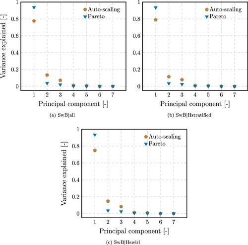
The variance explained by PC1 is in good agreement with the threshold proposed by Parente et al. [46]. Their study showed that by accounting for ∼0.9 of the total variance, all main species and temperature can be recovered with satisfactory levels of approximation. Consequently, the physical interpretation of all other principal components is omitted in this work, as is it believed to be out of the scope of this study.

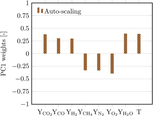
In order to determine the underlying structure of PC1, the weights of the original variables characterising the three databases (i.e. matrix A) are presented in Figure 3 for both scaling methods. Regardless of the scaling method used, it is interesting to note that PCA is able to automatically distinguish reactants from products, with PC1 being negatively and positively correlated with reactants and combustion products, respectively. Regardless of the data-set, it appears that the mass fractions of CO${}_2$ and O${}_2$ have the most important contributions to PC1-Pareto, and to a larger extent Y${}_{\mathrm{H}2\mathrm{O}}$, with coefficients equal to approximately 0.6, 0.65 and 0.35, respectively. This trend is also apparent for PC1-AS, with the latter having non-negligible weights on intermediate species, as opposed to Pareto, which clearly emphasises main species. This observation agrees with the study undertaken by Parente et al. [52] which has shown that the variance accounted for minor species by Auto-scaling is up to ∼20% higher than that explained by the other scaling methods investigated in their work.

Figure 3. Comparison of weights obtained with Pareto and Auto-scaling (with strips) for the leading principal component and scalars of (a) SwB$|$all, (b) SwB$|$Hstratified and (c) SwB$|$Hswirl.

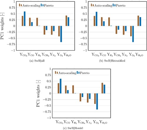
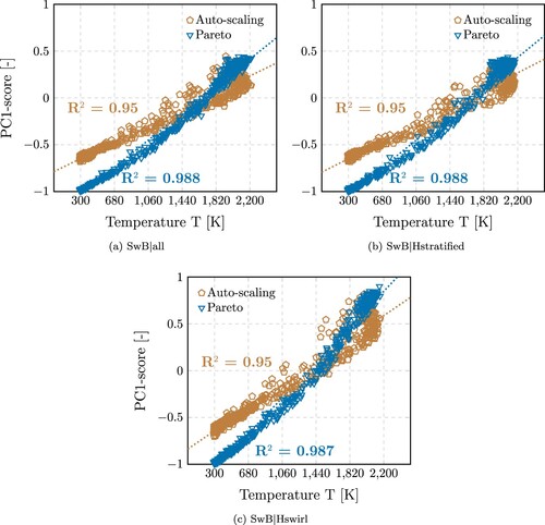
Considering the criterion proposed by Ranade & Echekki [53], only coefficients with magnitudes $\ge 0.4$ are kept to help identify the more prominent contributors to PC1. As PC1-Pareto, the same three species appear to have dominant weights on PC1-AS, namely the mass fractions of CO${}_2$, O${}_2$ and H${}_2$O, with ∼0.4. It is worth mentioning that all three scalars are known to behave linearly with temperature, thus suggesting that PC1 is perhaps correlated/aligned with temperature. This trend is illustrated in Figure 4, where results of all three data-sets considered herein promote a PC1 monotonically increasing with temperature. As expected, this behaviour is clearly accentuated by adopting the Pareto method.

Figure 4. Comparison of correlations obtained with Pareto (triangles) and Auto-scaling (pentagons) for the leading principal component with temperature for (a) SwB$|$all, (b) SwB$|$Hstratified and (c) SwB$|$Hswirl. The markers illustrate 500 point-based measurements randomly selected within the flames' and PC1-scores' data-sets.

A supplementary analysis was carried out by including temperature in SwB$|$all and using only Auto-scaling, as PC1-Pareto will be constrained to align with temperature. Figure 5 illustrates the dominant contributions to PC1-AS. The temperature scalar and the same three species mass fractions have the largest weights on PC1, with ∼0.4, suggesting that PC1, regardless of the scaling method adopted, is correlated with temperature.

Figure 5. Comparison of weights obtained with Auto-scaling (with strips) for the leading principal component and scalars of SwB$|$all with temperature included. PC1-AS accounts for ∼0.8 of the total variance, R${}^2=0.97$-AS with temperature.

After identifying the structure of the first principal component, the first-moment conditional fluctuations analysis of all three databases is carried out to investigate which of the proposed progress variables can sufficiently accurately characterise the composition space. As suggested by PCA, particular attention is brought to the temperature-based progress variable $c_1$.

3.2. All flames (SwB1-11)

Conditional averages of the Q variables describing the SwB$|$all thermo-chemical state can be calculated and consequently determine the conditional fluctuation associated with each experimental measurement. One-condition conditional averages using one of the four progress variables are investigated and compared to one another in order to determine the most optimal definition of $c_k$. Figure 6 illustrates the conditional fluctuations of temperature and five different species mass fractions. To clarify, throughout the entire document, figures with axial locations account for all data at different radial locations.

Figure 6. Conditional fluctuations of species mass fractions and temperature around the conditional average $〈f|\xi =c_k〉\left(x\right)$ for SwB$|$all database using only $c_k$ as the single conditioning variable and collecting all points at different radii together; are also shown the local average of these conditional fluctuations $〈f_{i,k}^{\mathrm{\prime }}〉$ (golden markers).

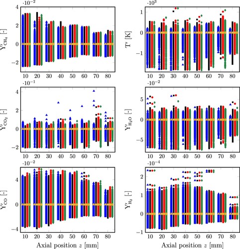
Regardless of the progress variable investigated, at all eight downstream locations, conditional fluctuations of the mass fraction of CH${}_4$, CO and H${}_2$ around $c_k$ exhibit an important functional dependence on the physical domain, stratification and/or swirl, visually highlighted by conditional fluctuation points spread far from zero. This trend is emphasised near the burner's tip, where the heat exchange with the bluff body might be significant, but also where an important recirculation of the flow is encountered. Due to high swirl, the recirculation zone is extended further downstream, leading to important conditional fluctuations of intermediate species at axial distances corresponding to z = 40, 50 mm. It is interesting to note that all investigated $c_k$ promote very similar results for the same three previous species. On the contrary, the conditional fluctuations of temperature and mass fractions of CO${}_2$ and H${}_2$O vary in function of the progress variable retained. The conditional fluctuations of Y${}_{\mathrm{H}2\mathrm{O}}$ around $c_1$ suggest that a temperature-based progress variable can perhaps more effectively decrease the functional dependence on the physical domain compared to the other $c_k$. This can be attributed to the fact that the mass fraction of H${}_2$O is closely relevant to temperature. As expected, a similar behaviour can be seen for the conditional fluctuations of T around $c_1$, and the conditional fluctuations of Y${}_{\mathrm{C}\mathrm{O}2}$ around $c_2$.

While local averages of all conditional fluctuations are anchored at zero, and thus, suggesting that all progress variables investigated are doing a good job of characterising the considered data-set, it is nearly impossible to find which definition of c is effectively the best choice to accurately describe the thermo-chemical state-space, and detach it from spatial coordinates, but also swirl and/or stratification effects.

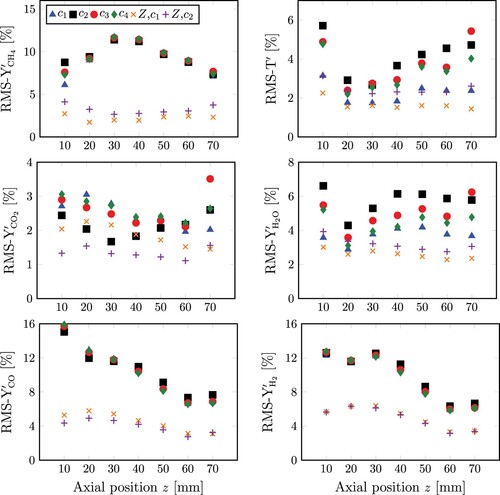
Figure 7 enables to distinct the performances of each $c_k$ by analysing each variable's normalised RMS. The normalised RMS of Y${}_{\mathrm{C}\mathrm{O}2}^{\mathrm{\prime }}$ around $c_2$ provides the best results due to the inclusion of the CO${}_2$ mass fraction in $c_2$. As expected, the same trend is observed for the RMS of T${}^{\mathrm{\prime }}$ around $c_1$. It is interesting to note that further downstream the axial position, the RMS of Y${}_{\mathrm{C}\mathrm{O}2}^{\mathrm{\prime }}$ around $c_1$ are improved or off the same order of magnitude as the Y${}_{\mathrm{C}\mathrm{O}2}$-based progress variable. Additionally, the RMS of Y${}_{\mathrm{C}\mathrm{H}4}^{\mathrm{\prime }}$ obtained using any $c_k$ are unchanged and remain close to 10%. Assuming that RMS of conditional fluctuations of the order of 10% can be considered as ‘relatively small’ [34], one can suppose that using a single conditioning variable for this database might still give acceptable predictions of the considered reactive scalar for conditional moment closure models.

Figure 7. Normalised RMS of the conditional fluctuations of temperature and species mass fractions for the SwB$|$all database around the conditional average $〈f|\xi =c_k〉\left(x\right)$ (markers) using $c_k$ as the single conditioning variable and around the conditional average $〈f|\eta =Z,\xi =c_1,c_2〉\left(x\right)$ using the mixture fraction and, the temperature-based progress variable (crosses) or the Y${}_{\mathrm{C}\mathrm{O}2}$-based progress variable (pluses), and collecting all points at different radii together.

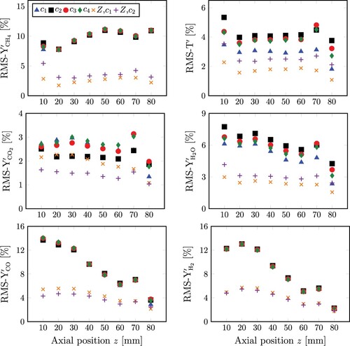
However, using $c_k$ as a single conditioning variable gives poor results for intermediate species, i.e. CO and H${}_2$, where normalised RMS exceed 10% of the maximum value of that particular scalar in the regions near the burner's tip. This suggests that the conditional averages are different (changing in function of space, stratification and/or swirl) and that a single controlling variable is not sufficient. The normalised RMS analysis contradicts the PCA results, where a single principal component direction was found to have the highest correlation with the reactive scalars. This is possibly due to the inherent nature of the PCA model, where PC-scores provide a rigorous mathematical formalism to reduce the dimensionality of the original data while retaining most of the variance induced by the turbulent fluctuations. Consequently, conditional fluctuations around two-condition conditional averages using mixture fraction and a temperature-based progress variable ($Z,c_1$) are considered in this study. Conditional fluctuations around mixture fraction and a Y${}_{\mathrm{C}\mathrm{O}2}$-based progress variable ($Z,c_2$) are also included to provide further insight. Each mixture fraction dimension is divided into 50 bins. It can be deduced that: (i) doubly conditioning is of particular interest for intermediate species, in particular those believed to be highly correlated with Z (e.g. Y${}_{\mathrm{C}\mathrm{O}}$), and (ii) regardless of the $c_k$ selected, one-condition conditional averages seem to not deviate that much from two conditions (e.g. temperature, carbon dioxide and water). Interestingly, normalised RMS of fluctuations around the one-condition conditional averages of Y${}_{\mathrm{C}\mathrm{O}}$ and Y${}_{\mathrm{H}2}$ are nearly as efficient as $Z,c_1$ and $Z,c_2$ further downstream the axial direction. The normalised RMS of major species and temperature using the mixture fraction and the temperature-based progress variable are somewhat more effective compared to $Z,c_2$, excluding, again, the RMS of Y${}_{\mathrm{C}\mathrm{O}2}^{\mathrm{\prime }}$. The differences remain minor, suggesting that the choice of a particular progress variable definition does not seem important, as deduced in [33]. However, it is believed that adopting Z and $c_1$ as the two controlling variables will provide a much more accurate representation of the Cambridge/Sandia flames' chemistry compared to mixture fraction and a species-based progress variable. The underlying assumption here is that diffusion effects play an essential role in describing the chemical states. From this perspective, it is assumed that c($Y_{\mathrm{i}}$) would be a poor choice as the diffusion coefficient is often modelled using the unity Lewis number assumption, whereas the reduced temperature progress variable includes the thermal diffusivity by solving the diffusion flux term. Recently, Turkeri et al. [54] showed through a parametric study that preferential diffusion is less relevant than heat losses for the studied burner, as it was found that the latter are more prevalent to accurately capture the underlying physics, particularly at the inlet of the burner.

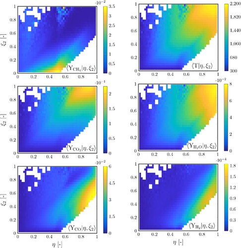
The two-condition conditional averages of the temperature and mass fractions of several species around mixture fraction and $c_1$ are shown in Figure 8. The obtained results are in good agreement with [40], where minor discrepancies are attributed to the different data-processing steps adopted in this study. The contours of conditionally-averaged scalars around Z and a Y${}_{\mathrm{C}\mathrm{O}2}$-based progress variable are illustrated in Figure 9. Despite gathering data from all axial and radial locations, one region common to both conditional domains can be identified in which no measurement has been found. Assuming the mixture fraction lies within the limits of flammability, the empty region suggests that the unburnt reactants are becoming unstable and start to react, such that methane is consumed and the progress variable rises. This trend is highlighted in both figures, where the mass fractions of CH${}_4$ peak near the lower flammability limit (i.e. Z = 0.575) of the methane-air mixture. It appears that adopting $c_1$ as a second control variable reduces the complete filling of the $\eta ,{\xi }_1$ space, as opposed to selecting a Y${}_{\mathrm{C}\mathrm{O}2}$-based progress variable. A second region without measurements is found in the conditional domain using Z and the temperature progress variable. The presence of the top-left region suggests that it is improbable to have a complete reaction with local equivalence ratios well below the lower flammability limit of methane. This behaviour is back-supported by Figure 9 where all conditionally-averaged scalars falling within this region are associated with values equal to zero. Interestingly, the conditional domain built using the mixture fraction and $c_2$ provides a much more complete mapping than $Z,c_1$, in particular for regions associated with high mixture fractions and progress variable values far from unity. The contours for conditionally-averaged temperature, CO${}_2$ mass fraction and H${}_2$O mass fraction exhibit, as expected, similar behaviours, where their maximum values lie in the vicinity of $Z_{\mathrm{s}\mathrm{t}}=0.9$ and progress variable of unity.

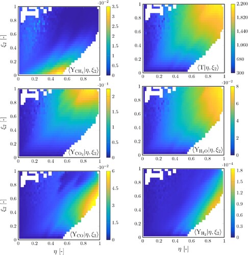
Figure 8. Two-condition conditionally averaged reactive scalars from SwB$|$all using η and ${\xi }_1$ as the sampling space variables of mixture fraction and the temperature-based progress variable $c_1$, respectively, and collecting data at all spatial locations (radial and axial). The temperature colourbar is expressed in Kelvin.

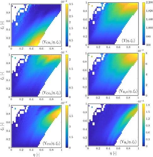
Figure 9. Two-condition conditionally averaged reactive scalars from SwB$|$all using η and ${\xi }_2$ as the sampling space variables of mixture fraction and the Y${}_{\mathrm{C}\mathrm{O}2}$-based progress variable $c_2$, respectively, and collecting data at all spatial locations (radial and axial). The temperature colourbar is expressed in Kelvin.

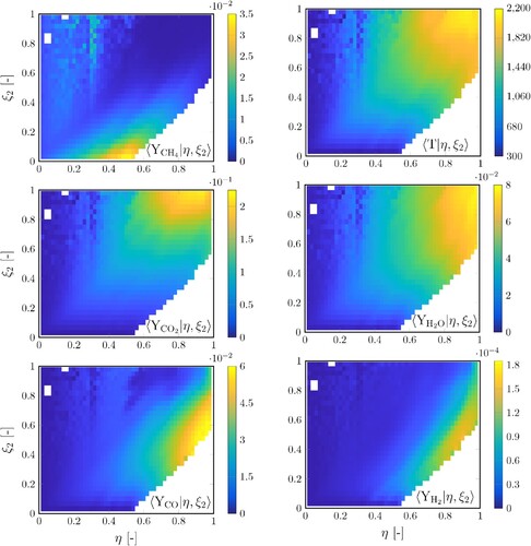
Figure 10. Normalised RMS of the conditional fluctuations of temperature and species mass fractions for the SwB$|$Hstratified database around the conditional average $〈f|\xi =c_k〉\left(x\right)$ (markers) using $c_k$ as the single conditioning variable and around the conditional average $〈f|\eta =Z,\xi =c_1,c_2〉\left(x\right)$ using the mixture fraction and, the temperature-based progress variable (crosses) or the Y${}_{\mathrm{C}\mathrm{O}2}$-based progress variable (pluses), and collecting all points at different radii together.

Intermediate species, namely CO and H${}_2$ mass fractions have similar behaviour in both conditional domains. However, it should be noted that using $c_2$ as a second control variable promotes a conditional mapping of regions associated with maximum values to be much more spread across $\eta ,{\xi }_2$, as opposed to the trends observed with Z and the temperature-based progress variable.

3.3. Fixed high stratification, swirl sweep (SwB9, SwB10, SwB11)

Within this section, the conditional fluctuations of the Q scalars describing SwB$|$Hstratified around one-condition conditional averages are studied to investigate which progress variable definition can reduce the swirl and spatial dependences, assuming high fixed stratification mixture conditions. The conditional fluctuations of temperature and various species mass fractions, depicted in Appendix 1 (cf. Figure A1), exhibit similar results compared to SwB$|$all. All studied $c_k$ promote similar behaviours for the conditional fluctuations of Y${}_{\mathrm{C}\mathrm{H}4}$, Y${}_{\mathrm{C}\mathrm{O}}$ and Y${}_{\mathrm{H}2}$. This suggests that the progress variable is perhaps not a good choice for describing the variables of interest and that mixture fraction would be a better decision, as the mass fractions of CH${}_4$ and CO are strongly correlated with Z. Moreover, the height of conditional fluctuations (in particular for intermediate species) seems to remain constant throughout all axial positions, as opposed to the trends observed with SwB$|$all. The local averages of the presented conditional fluctuations (cf. golden markers in Figure A1) are fixed at zero, suggesting that using either of the proposed $c_k$ as a conditioning variable should provide an accurate approximation of the turbulent reaction rate, i.e. a closure utilising only the first term of a Taylor expansion of the reaction rate.

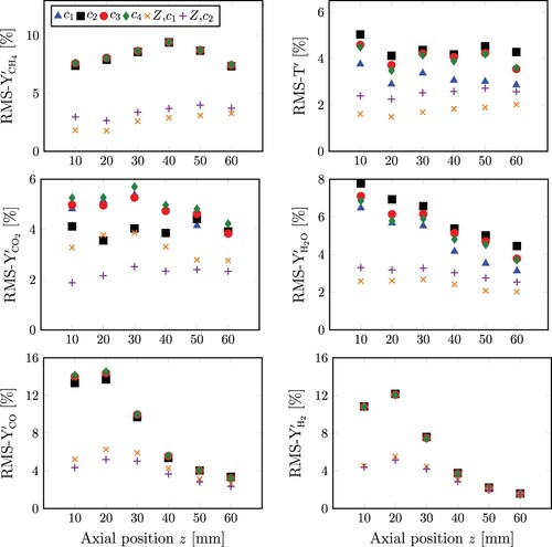
Figure 10 provides further insights. The normalised RMS of all variables investigated for the considered database around one-condition (i.e. using $c_k$) exhibit similar results as seen with SwB$|$all.

As expected, the RMS obtained using a single control variable have much higher swirl dependence at the inlet of the burner than two-condition conditional averages, in particular for methane, CO and H${}_2$ mass fractions, emphasised by normalised RMS values above 10%. Further downstream the axial direction (i.e. z = 60, 70 mm), the normalised RMS are nearly of the same order of magnitude as both combinations of doubly conditioning, suggesting that adding the mixture fraction as a second control variable does not significantly affect the fit. For the same species, the definition attributed to the progress variable seems irrelevant. The differences are more straightforward for major species and temperature, where all $c_k$ provide very good results. Based on these results, the temperature-based progress variable seems to be the most optimal choice (as concluded from the PCA analysis), followed by $c_4$ and $c_3$, and with the Y${}_{\mathrm{C}\mathrm{O}2}$-based progress variable being the worse among the tested reaction variables. These findings are consistent with recent results computed by analysing methane-air [55] and hydrogen-air [21] premixed flames. The normalised RMS around two-condition conditional averages are unchanged compared to the trends observed with the first database. The definition attributed to the progress variable as a second control scalar seems irrelevant for this case. Once again, two-condition conditional averages are sufficient to describe the considered database and detach it from swirl and space. This suggests that a DCSE calculation of these flames (including SwB$|$all) using both mixture fraction and progress variable as conditioning variables might be successful.

The contours of conditionally-averaged reactive scalars are illustrated in Appendix 1. The conditional averages of temperature and several species mass fractions around the mixture fraction and the temperature-based progress variable are shown in Figure A2. Figure A3 presents the conditional averages of the same scalars using Z and $c_2$. Similar conclusions drawn for SwB$|$all can be applied to the considered data-set. Regions with no available measurements are much more accentuated in both conditional domains, attributed to the exclusion of data from 6 flames that do not exhibit the desired characteristics of the current database. Regardless of the second control variable adopted, the conditional averaged scalars vary moderately throughout the two databases assessed, suggesting that the underlying physics and chemistry remain quasi-unchanged in the conditional domains.

3.4. Fixed high swirl, stratification sweep (SwB3, SwB7, SwB11)

The conditional fluctuations around one-condition conditional averages of the variables describing the SwB$|$Hswirl database are studied to investigate the most optimal choice of progress variable definition to cancel stratification and spatial dependences, assuming high fixed swirl intensity. The conditional fluctuations of the scalars previously investigated are shown in Appendix 2-Figure A4. Similar to SwB$|$all and SwB$|$Hstratified, the conditional fluctuations of Y${}_{\mathrm{C}\mathrm{H}4}$, Y${}_{\mathrm{C}\mathrm{O}}$ and Y${}_{\mathrm{H}2}$ appear to be still affected by space and stratification effects, particularly at the inlet of the burner. All $c_k$ promote similar results, suggesting that another choice of scalar is perhaps more suitable. Just like $c_2$ for Y${}_{\mathrm{C}\mathrm{O}2}^{\mathrm{\prime }}$, the temperature-based progress variable provide the lowest fluctuation heights for T${}^{\mathrm{\prime }}$ and Y${}_{\mathrm{H}2\mathrm{O}}^{\mathrm{\prime }}$, with $c_2$ and $c_3$ being the worse for the considered scalars. As in the two previous databases, the local averages throughout all downstream locations are equal to zero, suggesting that the definition attributed to the progress variable is perhaps less relevant in a closure context than in an accurate representation of the chemical state.

Surprisingly, Figure 11 shows that using a single conditioning variable for intermediate species, regardless of the definition attributed to c, equally well performs as Z,c(T) and Z,c($Y_{\mathrm{C}\mathrm{O}2}$), excluding the results obtained near the inlet of the burner (i.e. z = 10, 20 mm) where values deviate by a factor of ∼2, attributed to the recirculation zone and possibly the heat exchange with the bluff body. For these axial distances, this suggests that all investigated $c_k$ are enabling to decrease the functional dependence of conditional averages on spatial coordinates and stratification.

Figure 11. Normalised RMS of the conditional fluctuations of temperature and species mass fractions for the SwB$|$Hswirl database around the conditional average $〈f|\xi =c_k〉\left(x\right)$ (markers) using $c_k$ as the single conditioning variable and around the conditional average $〈f|\eta =Z,\xi =c_1,c_2〉\left(x\right)$ using the mixture fraction and, the temperature-based progress variable (crosses) or the Y${}_{\mathrm{C}\mathrm{O}2}$-based progress variable (pluses), and collecting all points at different radii together.

Moreover, compared to the two other data-sets, the normalised RMS of CH${}_4$ conditional fluctuations remain below 10%, suggesting that stratification effects have perhaps less influence on conditional averages than spatial coordinates and/or swirl. Differences of magnitude between the four $c_k$ are more pronounced for temperature and major species (excluding Y${}_{\mathrm{C}\mathrm{H}4}$), where $c_1$ provides the best fit for the mass fraction of H${}_2$O, but temperature as well (as expected). As was foreseeable, the inclusion of carbon dioxide in $c_2$ gives the most optimal results for decreasing the RMS of Y${}_{\mathrm{C}\mathrm{O}2}^{\mathrm{\prime }}$, with no apparent differences compared to other $c_k$ further downstream. The differences between the two combinations of doubly conditioning remain minor, with slightly better results in favour of $Z,c_1$, excluding the RMS of CO${}_2$ conditional fluctuations. This suggests that the definition attributed to the progress variable might be less relevant to conditional space fluctuations. This finding perhaps relates to the fundamental basis of conditional moment closure-based models where one focuses on the separation of model elements which give descriptions for the moment of reactive parameters concerning the scalar description in state-space. In that sense, the main purpose of the controlling variable is to construct a functional approximation of the conditional space where the number of control variables and their ability to capture major physical behaviour of the system (e.g. mixing and/or reaction progress) can be more relevant. This work, together with a previous study from Mousemi et al. [40], has indeed demonstrated the importance of including appropriate controlling variables to capture all physical processes and reduce conditional space fluctuations for reacting flows where the definition of progress variable can be more flexible. This perhaps has shown some differences compared to previous studies using one-dimensional (1D) flamelet models where a different progress variable using a simple linear combination of mass fraction definition resulted in significant differences in mass burning rate predictions [20]. One of the reasons identified by Gupta et al. is that when tabulated chemistry is constructed in 1D manifold approaches, a direct projection using control variables is involved, whereby the stretch and individual species transport phenomena in turbulent reactive flows might be neglected, resulting in significant differences in mass burning rate predictions [20]. Special treatment is therefore needed for the construction of a 1D manifold to reduce the impact of reaction progress variable choices via the projection of the source term and the diffusion term. Alternatively, extending the manifold dimension to properly account for mixing and chemical time scales can help account for variations in chemically conserved quantities such as element mass fractions [19]. This later study perhaps corresponds better with the results shown here in this work where, when two conditional variables are considered, the conditional fluctuations are significantly reduced irrespective of the choices of progress variables. However, a direct comparison with the above-mentioned studies is not available as the current study is based on experimental data measurements whereby the mass burning rate of the species is not available. Therefore the quantitative differences of progress variable choices in the context of turbulent combustion modelling using conditional moment closure approaches remain to be investigated.

Additionally, the contours of two-condition conditional averages have also been added in Appendix 2. The conditional averages of temperature and mass fractions of several species around mixture fraction and the temperature progress variable are shown in Figure A5. The conditionally-averaged scalars around Z and $c_2$ are illustrated in Figure A6. No apparent differences can be identified among the conditional domains computed from each of the three databases (assuming the use of the same two control variables), suggesting that the conditional averaged scalars behaviour is not affected by the underlying characteristics and effects of the studied burner.

4. Conclusion

Within this study, the Cambridge/Sandia swirl measurements are used in conjunction with principal component analysis (PCA) to attempt to find which set of control variables has the highest correlation with the reactive scalars. Three databases have been constructed to investigate the influence of swirl, stratification and spatial coordinates. Two scaling methods for the PCA model have been adopted, namely Pareto and Auto-scaling (AS). For all three data-sets, and regardless of the scaling method adopted, it was found that: (i) the first principal component (PC1) accounts for the largest amount of variance, and (ii) PC1 is well-aligned with temperature.

The conditional spaces of Cambridge/Sandia flames are examined by investigating the conditional fluctuations of temperature and various species mass fractions obtained with single-conditional averages around four different progress variable definitions. While conditional fluctuations of intermediate species and methane are unchanged using the progress variables tested, it was found that adopting a temperature-based progress variable provides minor improvements for major reactive scalars, in particular for temperature and H${}_2$O. For all three databases, the local averages of conditional fluctuations throughout all downstream locations are anchored at zero, suggesting that the definition attributed to the progress variable is perhaps less relevant in a closure context. Regardless of the data-set, the normalised RMS of the reactive scalars indicates that a single control variable based on c is unable to detach the thermo-chemical state from spatial coordinate, swirl or stratification, in particular for regions near the burner's tip characterised by an intense recirculation of the flow and significant heat exchanges with the bluff-body. The RMS analysis was followed by comparing the conditional averages obtained with the progress variables against doubly conditional averages using the mixture fraction and the progress variable c(T). Normalised RMS around two-condition conditional averages adopting mixture fraction and a Y${}_{\mathrm{C}\mathrm{O}2}$-based progress variable have also been included. Here, it was shown that the conditional fluctuations using both sets of two-condition conditional averages did not improve the dependence on the physical domain compared to a single progress variable condition further downstream the axial direction. The results are significantly improved at the burner inlet, with values not exceeding the 10% threshold used within this study as a guideline. The differences observed between both combinations of doubly conditioning are minor, suggesting that the choice of a particular progress variable definition does not seem to have an importance. Consequently, it is believed that a conditional moment closure calculation using both Z and c as two conditioning scalars might be successful, assuming that the ensemble has been divided along the axial direction. The conditional space fluctuations indicate that the success of CMC-based approaches does not depend on the definition attributed to the progress variable, which in fine increases the applicability of such models to different fuels and structures of flame. However, additional posterior research would be required for these flame configurations to obtain the mass burning rates using chemistry calculations, enabling a more rigorous/coherent comparison with previous studies given by other modelling approaches.

Following the PCA analysis results, and given that doubly conditioning seems to decrease the reactive scalars' dependence more effectively, it is suggested that c(T) could give a more accurate representation of the Cambridge/Sandia flames' chemistry (such as in a manifold) than a species-based progress variable, considering that species diffusivity is often simplified by assuming unity Lewis numbers. For future studies, other criteria may have to be tackled to evaluate the most suitable progress variable, such as the influence of heat losses, monotonicity, species recombination in post-combustion zones, and radiation effects. It should also be mentioned that the modelling of the joint probability density function (PDF) of mixture fraction and progress variable remains an important unresolved issue for CMC-based models, where the statistical independence assumption is anticipated to be invalid and how the definitions of progress variable affect joint-PDF also requires additional studies.

Acknowledgments

The authors wish to express gratitude to Professor Alessandro Parente for having provided the impulse to pursue the work presented here. His various suggestions for improvements of the work are greatly appreciated. Special thanks are given to Dr. M. S. Sweeney for the high-quality measurements of the Cambridge/Sandia swirl burner and for making them available to the community. Substantial thanks go to Professor Simone Hochgreb and Mr A. Mousemi who kindly share the full point-based measurements with the authors. The authors would also like to acknowledge the funding support from EPSRC Prosperity Partnership (EP/T005327/1). Dr XiaoHang Fang gratefully acknowledges the financial support provided by the Department of Engineering Science, University of Oxford during the completion of this work. This publication also arises from research funded by the John Fell Oxford University Press Research Fund and the NSERC Discovery Grant (RGPIN-2023-03309).

Disclosure statement

No potential conflict of interest was reported by the author(s).

Additional information

Funding

This work was supported by Engineering and Physical Sciences Research Council[EP/T005327/1] John Fell Fund, University of Oxford[0010894]  and Natural Sciences and Engineering Research Council of Canada [RGPIN-2023-03309].

Appendices

Appendix 1.

SwB$|$Hstratified

Figure A1. Conditional fluctuations of species mass fractions and temperature around the conditional average $〈f|\xi =c_k〉\left(x\right)$ for SwB$|$Hstratified database using only the progress variable as the single conditioning variable and collecting all points at different radii together; are also shown the local average of these conditional fluctuations $〈f_{i,k}^{\mathrm{\prime }}〉$ (golden markers).

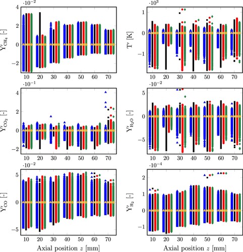
Figure A2. Two-condition conditionally averaged reactive scalars from SwB$|$Hstratified using η and ${\xi }_1$ as the sampling space variables of mixture fraction and the temperature-based progress variable $c_1$, respectively, and collecting data at all spatial locations (radial and axial). The temperature colourbar is expressed in Kelvin.

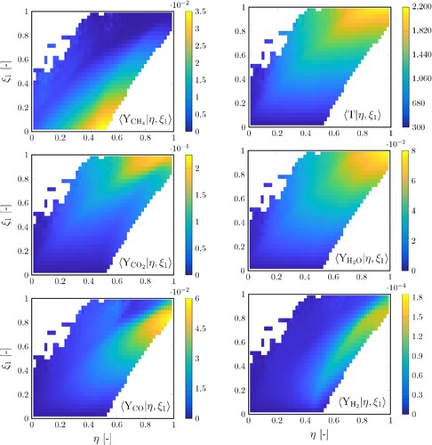
Figure A3. Two-condition conditionally averaged reactive scalars from SwB$|$Hstratified using η and ${\xi }_2$ as the sampling space variables of mixture fraction and the Y${}_{\mathrm{C}\mathrm{O}2}$-based progress variable $c_2$, respectively, and collecting data at all spatial locations (radial and axial). The temperature colourbar is expressed in Kelvin.

Appendix 2.

SwB$|$Hswirl

Figure A4. Conditional fluctuations of species mass fractions and temperature around the conditional average $〈f|\xi =c_k〉\left(x\right)$ for SwB$|$Hswirl database using only the progress variable as the single conditioning variable and collecting all points at different radii together; are also shown the local average of these conditional fluctuations $〈f_{i,k}^{\mathrm{\prime }}〉$ (golden markers).

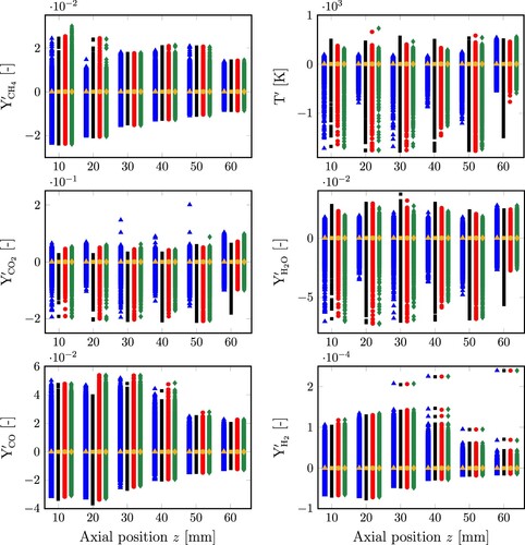
Figure A5. Two-condition conditionally averaged reactive scalars from SwB$|$Hswirl using η and ${\xi }_1$ as the sampling space variables of mixture fraction and the temperature-based progress variable $c_1$, respectively, and collecting data at all spatial locations (radial and axial). The temperature colourbar is expressed in Kelvin.

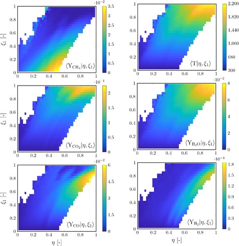
Figure A6. Two-condition conditionally averaged reactive scalars from SwB$|$Hswirl using η and ${\xi }_2$ as the sampling space variables of mixture fraction and the Y${}_{\mathrm{C}\mathrm{O}2}$-based progress variable $c_2$, respectively, and collecting data at all spatial locations (radial and axial). The temperature colourbar is expressed in Kelvin.

References

- J. van Oijen, A. Donini, R. Bastiaans, J. ten Thije Boonkkamp, and L. de Goey, State-of-the-art in premixed combustion modeling using flamelet generated manifolds, Prog. Energy. Combust. Sci. 57 (2016), pp. 30–74.
- A. Klimenko and R. Bilger, Conditional moment closure for turbulent combustion, Prog. Energy. Combust. Sci. 25 (1999), pp. 595–687.
- D. Veynante and L. Vervisch, Turbulent combustion modeling, Prog. Energy. Combust. Sci. 28 (2002), pp. 193–266.
- T. Poinsot and D. Veynante, Theoretical and numerical combustion, 2nd ed., RT Edwards, Philadelphia PA, 2005.
- D. Dovizio, J.W. Labahn, and C.B. Devaud, Doubly conditional source-term estimation (DCSE) applied to a series of lifted turbulent jet flames in cold air, Combust. Flame.162 (2015), pp. 1976–1986.
- P.D. Nguyen, L. Vervisch, V. Subramanian, and P. Domingo, Multidimensional flamelet-generated manifolds for partially premixed combustion, Combust. Flame. 157 (2010), pp. 43–61.
- A.H. Mahdipour and M.M. Salehi, Localized conditional source-term estimation model for turbulent combustion, Combustion Flame. 235 (2021), p. 111715.
- M. Ihme and Y.C. See, LES flamelet modeling of a three-stream MILD combustor: analysis of flame sensitivity to scalar inflow conditions, Proc. Combustion Inst. 33 (2011), pp. 1309–1317.
- M. Ihme, J. Zhang, G. He, and B. Dally, Large-Eddy simulation of a Jet-in-Hot-Coflow burner operating in the Oxygen-Diluted combustion regime, Flow, Turbulence Combustion 89 (2012), pp. 449–464.
- J. Labahn, D. Dovizio, and C. Devaud, Numerical simulation of the Delft-Jet-in-Hot-Coflow (DJHC) flame using conditional source-term estimation, Proc. Combustion Inst. 35 (2015), pp. 3547–3555.
- J. Labahn and C. Devaud, Large Eddy simulations (LES) including conditional source-term estimation (CSE) applied to two Delft-Jet-in-Hot-Coflow (DJHC) flames, Combust. Flame.164 (2016), pp. 68–84.
- R.W. Bilger and S.H. Starner, On reduced mechanisms for methane-air combustion in nonpremixed flames, Combust. Flame. 80 (1990), pp. 135–149.
- X. Fang, R. Ismail, M.H. Davy, and J. Camm, Numerical Studies of Combustion Recession on ECN Diesel Spray A, Internal Combustion Engine Division Fall Technical Conference Vol. 2: Emissions Control Systems; Instrumentation, Controls, and Hybrids; Numerical Simulation; Engine Design and Mechanical Development, Proceedings of the ASME 2018 Internal Combustion Engine Division Fall Technical Conference, San Diego, USA, Vol. 11, 2018, p. v002T06A011.
- X. Fang, R. Ismail, and M. Davy, A study on kinetic mechanisms of diesel fuel surrogate n-dodecane for the simulation of combustion recession, in WCX SAE World Congress Experience, SAE International, Detroit, 2019.
- Z. Sun, S. Gierth, M. Pollack, C. Hasse, and A. Scholtissek, Ignition under strained conditions: unsteady flamelet progress variable modeling for diesel engine conditions in the transient counterflow configuration, Combust. Flame. 240 (2022), p. 111841.
- M. Ihme, L. Shunn, and J. Zhang, Regularization of reaction progress variable for application to flamelet-based combustion models, J. Comput. Phys. 231 (2012), pp. 7715–7721.
- Y.S. Niu, L. Vervisch, and P.D. Tao, An optimization-based approach to detailed chemistry tabulation: automated progress variable definition, Combust. Flame. 160 (2013), pp. 776–785.
- A. Vasavan, P. de Goey, and J. van Oijen, A novel method to automate FGM progress variable with application to igniting combustion systems, Combustion Theory Modell. 24 (2020), pp. 221–244.
- F. Chitgarha, F. Ommi, and M. Farshchi, Assessment of optimal reaction progress variable characteristics for partially premixed flames, Combustion Theory Modell. 26 (2022), pp. 797–830.
- H. Gupta, O.J. Teerling, and J.A. van Oijen, Effect of progress variable definition on the mass burning rate of premixed laminar flames predicted by the flamelet generated manifold method, Combustion Theory Modell. 25 (2021), pp. 631–645.
- A. Lipatnikov and V. Sabelnikov, Evaluation of mean species mass fractions in premixed turbulent flames: a DNS study, Proc. Combustion Inst. 38 (2021), pp. 6413–6420.
- A. Lipatnikov, V. Sabelnikov, F. Hernández-Pérez, W. Song, and H.G. Im, A priori DNS study of applicability of flamelet concept to predicting mean concentrations of species in turbulent premixed flames at various Karlovitz numbers, Combust. Flame. 222 (2020), pp. 370–382.
- A. Giusti and E. Mastorakos, Detailed chemistry LES/CMC simulation of a swirling ethanol spray flame approaching blow-off, Proc. Combustion Inst. 36 (2017), pp. 2625–2632.
- A. Varna, A. Wehrfritz, E.R. Hawkes, M.J. Cleary, T. Lucchini, G. D'Errico, S. Kook, and Q.N. Chan, Application of a multiple mapping conditioning mixing model to ECN spray A, Proc. Combustion Inst.37 (2019), pp. 3263–3270.
- W.K. Bushe and H. Steiner, Conditional moment closure for large eddy simulation of nonpremixed turbulent reacting flows, Phys. Fluids 11 (1999), pp. 1896–1906.
- J.W. Labahn, I. Stanković, C.B. Devaud, and B. Merci, Comparative study between conditional moment closure (CMC) and conditional source-term estimation (CSE) applied to piloted jet flames, Combust. Flame. 181 (2017), pp. 172–187.
- Z. Huang, M.J. Cleary, Z. Ren, and H. Zhang, Large Eddy simulation of a supersonic lifted hydrogen flame with sparse-Lagrangian multiple mapping conditioning approach, Combustion Flame. 238 (2021), p. 111756.
- X. Fang, R. Ismail, K. Bushe, and M. Davy, Simulation of ECN diesel spray A using conditional source-term estimation, Combustion Theory Modell. 24 (2020), pp. 725–760.
- X. Fang, R. Ismail, N. Sekularac, and M. Davy, On the Prediction of Spray A End of Injection Phenomenon Using Conditional Source-Term Estimation, WCX SAE World Congress Experience, SAE International, Detroit, 2020.
- X. Fang, N. Sekularac, and M.H. Davy, Parametric Studies of a Novel Combustion Modelling Approach for Low Temperature Diesel Spray Simulation, Proceedings of the ASME 2020 Internal Combustion Engine Division Fall Technical Conference, 2020, p. v001T06A005.
- A. Hussien and C. Devaud, Simulations of partially premixed turbulent ethanol spray flames using doubly conditional source term estimation (DCSE), Combustion Flame. 239 (2021), p. 111651.
- D. Dovizio and C. Devaud, Doubly conditional source-term estimation (DCSE) for the modelling of turbulent stratified V-shaped flame, Combust. Flame. 172 (2016), pp. 79–93.
- C. Devaud, W.K. Bushe, and J. Bellan, The modeling of the turbulent reaction rate under high-pressure conditions: A priori evaluation of the conditional source-term estimation concept, Combust. Flame. 207 (2019), pp. 205–221.
- W. Bushe, Spatial gradients of conditional averages in turbulent flames, Combust. Flame. 192 (2018), pp. 314–339.
- A. Mousemi and W. Kendal Bushe, The joint probability density function of mixture fraction, reaction progress variable, and total enthalpy in a stratified, swirl-stabilized turbulent flame, Phys. Fluids 33 (2021), p. 035106.
- W.K. Bushe, C. Devaud, and J. Bellan, A priori evaluation of the double-conditioned conditional source-term estimation model for high-pressure heptane turbulent combustion using DNS data obtained with one-step chemistry, Combust. Flame. 217 (2020), pp. 131–151.
- J.C. Sutherland and A. Parente, Combustion modeling using principal component analysis, Proc. Combustion Inst. 32 (2009), pp. 1563–1570.
- M.S. Sweeney, S. Hochgreb, M.J. Dunn, and R.S. Barlow, The structure of turbulent stratified and premixed methane/air flames I: non-swirling flows, Combust. Flame. 159 (2012), pp. 2896–2911.
- M.S. Sweeney, S. Hochgreb, M.J. Dunn, and R.S. Barlow, The structure of turbulent stratified and premixed methane/air flames II: swirling flows, Combust. Flame. 159 (2012), pp. 2912–2929.
- A. Mousemi, W.K. Bushe, and S. Hochgreb, Evaluation of manifold representations of chemistry in stratified, swirl-stabilized flames, Combust. Flame. 229 (2021), p. 111418.
- M. Wang, J. Huang, and W. Bushe, Simulation of a turbulent non-premixed flame using conditional source-term estimation with trajectory generated low-dimensional manifold, Proc. Combustion Inst.31 (2007), pp. 1701–1709.
- O. Owoyele, P. Kundu, M.M. Ameen, T. Echekki, and S. Som, Application of deep artificial neural networks to multi-dimensional flamelet libraries and spray flames, Int. J. Engine Res. 21 (2020), pp. 151–168.
- M. Ihme, W.T. Chung, and A.A. Mishra, Combustion machine learning: principles, progress and prospects, Prog. Energy. Combust. Sci. 91 (2022), p. 101010.
- H. Mirgolbabaei and T. Echekki, Nonlinear reduction of combustion composition space with kernel principal component analysis, Combust. Flame. 161 (2014), pp. 118–126.
- M.R. Malik, P. Obando Vega, A. Coussement, and A. Parente, Combustion modeling using principal component analysis: a posteriori validation on sandia flames D, E and F, Proc. Combustion Inst. 38 (2021), pp. 2635–2643.
- A. Parente, J. Sutherland, L. Tognotti, and P. Smith, Identification of low-dimensional manifolds in turbulent flames, Proc. Combustion Inst. 32 (2009), pp. 1579–1586.
- J. Shlens, A tutorial on principal component analysis, 2014.
- B.J. Isaac, A. Coussement, O. Gicquel, P.J. Smith, and A. Parente, Reduced-order PCA models for chemical reacting flows, Combust. Flame. 161 (2014), pp. 2785–2800.
- A. Biglari and J.C. Sutherland, An a-posteriori evaluation of principal component analysis-based models for turbulent combustion simulations, Combust. Flame. 162 (2015), pp. 4025–4035.
- B.J. Isaac, J.N. Thornock, J. Sutherland, P.J. Smith, and A. Parente, Advanced regression methods for combustion modelling using principal components, Combust. Flame. 162 (2015), pp. 2592–2601.
- M.R. Malik, B.J. Isaac, A. Coussement, P.J. Smith, and A. Parente, Principal component analysis coupled with nonlinear regression for chemistry reduction, Combust. Flame.187 (2018), pp. 30–41.
- A. Parente and J.C. Sutherland, Principal component analysis of turbulent combustion data: data pre-processing and manifold sensitivity, Combust. Flame. 160 (2013), pp. 340–350.
- R. Ranade and T. Echekki, A framework for data-based turbulent combustion closure: A priori validation, Combust. Flame. 206 (2019), pp. 490–505.
- H. Turkeri, X. Zhao, and M. Muradoglu, Large eddy simulation/probability density function modeling of turbulent swirling stratified flame series, Phys. Fluids 33 (2021), p. 025117.
- A.N. Lipatnikov, T. Nilsson, R. Yu, X.S. Bai, and V.A. Sabelnikov, Assessment of a flamelet approach to evaluating mean species mass fractions in moderately and highly turbulent premixed flames, Phys. Fluids 33 (2021), p. 045121.