Reasoning cartographic knowledge in deep learning-based map generalization with explainable AI

Abstract

Cartographic map generalization involves complex rules, and a full automation has still not been achieved, despite many efforts over the past few decades. Pioneering studies show that some map generalization tasks can be partially automated by deep neural networks (DNNs). However, DNNs are still used as black-box models in previous studies. We argue that integrating explainable AI (XAI) into a DL-based map generalization process can give more insights to develop and refine the DNNs by understanding what cartographic knowledge exactly is learned. Following an XAI framework for an empirical case study, visual analytics and quantitative experiments were applied to explain the importance of input features regarding the prediction of a pre-trained ResU-Net model. This experimental case study finds that the XAI-based visualization results can easily be interpreted by human experts. With the proposed XAI workflow, we further find that the DNN pays more attention to the building boundaries than the interior parts of the buildings. We thus suggest that boundary intersection over union is a better evaluation metric than commonly used intersection over union in qualifying raster-based map generalization results. Overall, this study shows the necessity and feasibility of integrating XAI as part of future DL-based map generalization development frameworks.

Keywords:

• Map generalization
• XAI
• deep learning
• raster
• U-Net

1. Introduction

Cartographers typically learn explicit and implicit map generalization rules via examples that are summarized from general cartographic principles and practices (Swiss Society of Cartography 2005). Cartographers also have to make tradeoffs in certain scenarios concerning the spatial layout of maps and graphic constraints, such as visual perceptibility limits. Not surprisingly, then, research on automating the map generalization process has been largely dominated by the challenge to find ways of formalizing and translating the tacit cartographic knowledge possessed by trained cartographers into automated procedures. This process is vividly documented in several review articles and edited works spanning more than four decades of map generalization research until the developments of the recent past (Brassel and Weibel 1988, Müller et al. 1995, Weibel and Dutton 1999, Mackaness et al. 2007, Burghardt et al. 2014, Harrie et al. 2024). Starting off from the early years where the cartographic principles were built directly into the algorithms, to the rule-based systems of the 1980s, the principle of constraint-based map generalization was introduced in the 1990s, offering added modeling flexibility compared to rule-based systems (Beard 1991, Weibel and Dutton 1998, Harrie 1999). The constraint-based approach was subsequently complemented by the introduction of optimization approaches (Wilson et al. 2003, Bader et al. 2005, Sester 2005) and by systems allowing the orchestration of multiple generalization operators to form a comprehensive map generalization process, exemplified by the agent-based paradigm (Barrault et al. 2001, Ruas and Duchêne 2007). However, while this combination of constraint-based methods with optimization techniques and orchestration engines represented the state of the art for almost two decades, the above methods all suffered from one decisive drawback: The imperative necessity of formalizing the cartographic knowledge required to define constraints, develop algorithms, and fine-tune optimization and orchestration processes, ultimately slowing down progress in map generalization research (Weibel et al. 1995).

Deep learning (DL, LeCun et al. 2015) has increasingly shown itself as a new research paradigm for many GIScience studies and is regarded as a backbone of GeoAI today (Janowicz et al. 2020). It offers a potential way to overcome the so-called ‘knowledge acquisition bottleneck’ (Weibel et al. 1995) in which previous approaches mentioned above were trapped. In the research domain of map generalization, there have already been various applications using deep neural networks (DNNs) for automating map generalization tasks, such as selection (Xiao et al. 2023, Zheng et al. 2021), simplification (Du et al. 2022, Zhou et al. 2022), and even end-to-end solutions for buildings (Feng et al. 2019) and roads (Courtial et al. 2023).

While DNNs have achieved initial success in some map generalization tasks, the trained neural networks are still treated as black boxes where researchers have not explored what exact cartographic generalization knowledge the network has learned in what circumstances and which cartographic rules the network should improve on. Knowing to what degree a certain map generalization operator has been learned by a certain DNN architecture will enhance the decision-making on module selection in existing DL-based map generalization workflows such as DeepMapScaler (Courtial et al. 2024) or will help to propose new DL-based generalization models (Harrie et al. 2024). It has been argued that GeoAI should not be purely data-driven, but that the interpretability and explainability of the DNNs should also be considered (Janowicz et al. 2022, Hu et al. 2024). Lacking necessary explainability is also regarded as a major concern for DL models by some authors (Kang et al. 2024), as understanding the decision-making process is even more critical for DL-based map generalization due to the importance of maps.

Explainable AI (XAI, Arrieta et al. 2020) is a research field focusing on understanding the decisions made by AI systems by providing the necessary interpretations and explanations. It has been applied to reason about deep learning-related studies in scientific fields such as medical image analysis (van der Velden et al. 2022). Moreover, XAI is being integrated into the DL development workflow, forming an emerging field named explanation-guided learning (EGL) with the aim of developing more powerful and accountable DL models (Gao et al. 2024). While XAI already provides a general framework with a handful of analytical tools, the EGL community criticizes that current XAI tools lack attention to investigating if the explanations that are produced are indeed reasonable. Thus, domain knowledge is still required in response to this criticism. It also echoes the suggestion by Xing and Sieber (2021) that not all XAI methods are suitable for GeoAI applications as some XAI methods ignore or blur geographical dependencies.

Despite of the importance of XAI in developing domain-specific DNNs, few studies have attempted to uncover DNNs’ functional roles in the process of map generalization. Courtial et al. (2022) inspected how DL model outputs satisfy a set of cartographic constraints in a mountain road generalization task. However, they have not yet further investigated the fine-grained effects of input images on learning to generalise roads. As a consequence, one set of essential questions is, how do different elements of the input sample, that is, pixels for raster-based input and nodes and edges for graph-based input, contribute to making the decision on the output, in the eyes of a DNN? For such purposes, a workflow for a more explicit interpretation or explanation of the cartographic knowledge learned by the DNN itself would be highly desired (Harrie et al. 2024).

By emphasizing the necessity of integrating XAI into the current DL-based map generalization workflow, we demonstrate with a use case in building generalization how a suitable XAI method can be used to visually and quantitatively highlight and interpret the importance of individual pixels in the input raster map patch to generating the corresponding output map patch. This use case is based on a well-trained DNN for building generalization from a previous study (Fu et al. 2023). We further explore if such importance, representing the cartographic knowledge learned by the DNN, varies across map generalization samples involving different map generalization operators. With the proposed workflow guided by XAI, we further argue that the boundary intersection-over-union (Boundary IoU, Bokhovkin and Burnaev 2019, Cheng et al. 2021, Kervadec et al. 2021) may be a better evaluation metric than the widely used intersection-over-union (IoU), showing that the workflow has the potential to refine the DL-based learning task in map generalization by integrating cartographic knowledge with XAI.

2. Related work

2.1. Deep learning in map generalization

Researchers have made various attempts to generalize maps with DNNs for cartographic object classes such as buildings, roads, and rivers, with either vector- or raster-based models. For vector-based data models, graph convolutional networks (GCN, Kipf and Welling 2019) are the most prevalent DL architecture. Researchers have applied GCN models for building shape recognition (Yan et al. 2020) and building grouping (Yan et al. 2022). In vector-based DL models, cartographic knowledge is mainly engaged in the feature engineering stage. The aforementioned studies extracted geometric features related to distance and angle and represented them as node and edge features of the graphs. Studies have also tried an autoencoder for line simplification (Yu and Chen 2022), for which no prior cartographic knowledge is required for model training.

A big challenge for vector-based neural networks is that the spatial relationships of multiple polygonal objects such as buildings forming groups are not genuinely and easily modeled. Current application either limits their scope to a single object (Zhou et al. 2023) or represents polygonal objects by point objects (Xiao et al. 2023) for further modeling. A general-purpose representation of polygonal objects using embedding might be a solution, but only limited studies exist in this direction (Mai et al. 2022).

Raster-based DL for map generalization is treated as a type of image-to-image translation, typically utilizing generative models such as U-Net (Feng et al. 2019) or Generative Adversarial Networks (Courtial et al. 2023). With convolutional operators in DL models and genuine location encoding in the raster data, raster-based DL models can model the spatial relationships between polygonal objects (Courtial et al. 2022). However, the models cannot maintain well the topology of roads (Courtial et al. 2023). As raster-based DL models operate on pixels, shape irregularities may be introduced to building walls and corners. The deformation effect can be moderated with a layered data representation model (Fu et al. 2023). In raster-based DL studies, cartographic knowledge is represented either as items in the loss function (Kang et al. 2020, Courtial et al. 2023) or as part of the data representation model (Courtial et al. 2022, Fu et al. 2023). However, it is not fully understood whether and how a DL neural network has actually learned the desired knowledge.

2.2. XAI applications in DL-based GIScience

XAI aims to increase fairness, explainability, and accountability with technical tools and the involvement of end users, with a scope not only limited to DL but also other machine learning techniques (Arrieta et al. 2020). The techniques for interpreting raster-based DL models can be coarsely categorized into primary-, neuron-, and layer attributions, where primary attribution tries to attribute decisions of the whole neuron network to input features; neuron attribution attributes individual neurons to input features, and layer attribution links decisions of the whole network to a hidden layer (Kokhlikyan et al. 2020).

Primary attribution, as used in this study, mainly assumes the trained neural network as a linear transformation system and explores the gradient of output regarding the input, e.g. saliency (Simonyan et al. 2014); the gradients with regard to inputs along a path from a baseline input to the actual input, e.g. integrated gradients (Sundararajan et al. 2017); or the gradient w.r.t. small changes introduced in the input, e.g. DeepLIFT (Shrikumar et al. 2017).

Combined with visual analytics and other inspection tools, the XAI attribution methods can help researchers investigate the decision-making process of DNNs. There have been pioneering studies in GIScience. For example, Hasanpour Zaryabi et al. (2022) apply the aforementioned primary attribution tools to understand which pixels in an input satellite image contribute to building extraction results for a U-Net. Li et al. (2023) use various primary attribution tools to understand how traffic flows in different regions of a city contribute to the overall traffic prediction made by a U-Net. Similar workflows have also been used to understand the importance of satellite image bands in water depth estimation (Saeidi et al. 2023), pixel-level importance for land use classification (Xing and Sieber 2023), and terrain image classification (Hsu and Li 2023). Even though these studies are not in the field of cartography, coincidently, they also adopted raster-based DNNs, suggesting that similar methods can be used for explaining raster-based DL models for map generalization.

3. Research gaps and research question

In summary, many pioneering studies have been implemented to solve map generalization problems with deep neural networks as a new paradigm in recent years. Most studies adapted existing DNN architectures with intuitive improvement ideas related to existing map generalization knowledge but interacted with the neural networks as black boxes. However, configuring DNNs usually is highly complex, including network types, number of blocks, layer structures of the blocks, and loss function(s), leading to very large combinations of configuration settings. Training and testing each new configuration setting can be costly in time, which has drawn concern for sustainability in the GeoAI community as well (Shi et al. 2023). For further sustained efficiency and scientific improvement, one solution is to follow more evidence-based guidance using XAI and gradually adopt the EGL approach, so that future models can focus on tasks that have not been well learned by the existing models. However, so far very few studies in DL-based map generalization have tried this direction to gain improved scientific insight and to enhance DNNs with XAI.

Attempting to adapt XAI in the process of DL-based map generalization, this study shifts the focus from pursuing higher performance to exploring how the neural network learns particular cartographic insights. In a previous study, we proposed a U-Net-based map generalization workflow for raster-based map patches that showed promise for adequate results in building generalization (Fu et al. 2023). However, our improvement in the previous study was solely based on an intuitive idea, and there are many possibilities for improving the model. As a use case of integrating XAI in deep learning workflow for map generalization, we thus address one specific research question based on the challenges remaining in the previous study:

RQ: Which pixels, individually or structurally, in a raster-based input map patch of buildings are important to the generalized map patch, as learned by the deep neural network?

It has been well established that geometric shapes have a low-dimensional structure, meaning that drawing a polygonal shape can be controlled by the locations of its vertices and the shapes of its edges without concerning its interior, as being applied by many computer vision packages such as OpenCV (Bradski 2000). That is to say, to describe a raster representation of a polygonal shape, its corner and edge pixels are more important than its interior pixels. As the map generalization of buildings can be conceptualized as a transformation between two sets of rasterized polygonal shapes, we can raise a hypothesis that the pixels forming the boundary of the input building(s) contribute more than the interior pixels inside the building(s) to a DNN’s decision making regarding the generation of the output, that is, the generalized building(s). In addition to the buildings themselves, we further hypothesize that the space between the building objects is also important for determining the effort of selecting map generalization operators. For example, a minimum visual separation distance is employed by cartographers to ensure two buildings can be visually discerned on a generalized map. If the two buildings are too close, they may have to be aggregated into a single polygon for a map at a smaller scale. We thus will also investigate if the DL neural network recognizes such patterns.

4. Methodology

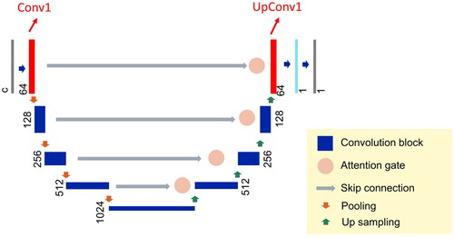
4.1. A Pre-trained ResU-Net model

The pre-trained DNN we try to explore is a ResU-Net (Zhang et al. 2018) that was trained with raster-based building map patches (Figure 1). The buildings were derived from OSM vector data in Stuttgart, Germany by Feng et al. (2019). The generalization transformations are from 1:5k to 1:10k, processed by the map generalization software CHANGE (Powitz 1993) with its simplification and combination (aggregation) operators. The ResU-Net model receives a 256*256-pixel binary input tensor with two channels whose first channel (Channel 0) stores the focal building that should be generated, and the second channel (Channel 1) stores the surrounding buildings of the focal building. The pre-trained model achieved an average accuracy of 0.9954 and an average intersection-over-union (IoU) of 0.9659 for individual buildings. Therefore, it is reasonable to conclude that the pre-trained model should have learned relevant cartographic map generalization knowledge, and that it thus can be used as a reliable instance supporting this case study to demonstrate the possible role of XAI in DL-based map generalization and answer our research question by testing the above hypothesis. Full technical details of the pre-trained model can be found in (Fu et al. 2023).

Figure 1. Architecture of the pre-trained U-Net, where c is the number of channels, and the convolution blocks in red are the blocks inspected in this study.

4.2. XAI for input feature importance exploration

The XAI tools selected are layer activation for reasoning about the responses of neural layers, and integrated gradients (IG, Sundararajan et al. 2017) for reasoning about input feature importance.

Layer activation focuses on what kind of output is produced by each neural layer or a set of neural layers, and visual analytics is commonly applied to interpret the results (Larochelle et al. 2009). The convolution blocks in a ResU-Net are a sequential combination of convolution layer, batch-wise normalization layer, and ReLU layer. The convolution blocks close to the input are supposed to act as encoders to extract higher dimensional features from the input, while the convolution blocks close to the output are supposed to combine the extracted features to reconstruct the image. Therefore, by visualizing the output of a convolution block, we are able to reason what features, as reflected in a combined way, are focused on by the inspected convolution block. We investigated the down-sampling convolution block closest to the input, and the up-sampling convolution block closest to the output (denoted as Conv1 and UpConv1 in Figure 1, respectively), because they are paired and have 64 dimensions, a reasonable number to conduct a close visual inspection.

Intuitively, IG uses gradients of the items along a straight-line path (Figure 1 in Sundararajan et al. 2017) from the input tensor to a baseline tensor as a proxy for individual items’ influences on the output, which can be formulated as: $$\mathit{\text{IntegratedGradient}}\left(x\right)\colon\colon =(x_i-x_i^{\prime })\times {\int }_{\alpha =0}^1\frac{\partial F(x\prime +\alpha \times (x-x\prime \left)\right)}{\partial x_i}d\alpha$$ where $x$ is the input tensor, $x\prime$ is the corresponding baseline, $F$ is the trained neural network, and $i$ is one dimension of the tensor (Sundararajan et al. 2017).

IG models the gradients as a function of sensitivity to the presence of the input features. Thus, IG needs a baseline tensor with the same shape as the input tensor so that the status between the input and the baseline tensor can be interpolated and the sensitivity can be obtained. The baseline should satisfy the condition that the DNN’s prediction using the baseline as input should be neutral. For the image-based object recognition task of the original paper the authors suggest a full black image as the baseline. The output of the IG algorithm is a tensor with the same shape as the input tensor. Because our input tensor is a layered representation that separates the focal building from the surrounding buildings, we expected that the influences of each input channel would be demonstrated in the corresponding channels of the output tensor.

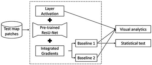
Following the analytical workflow for the building generalization tasks (Figure 2), we tried two baselines for the integrated gradient analysis: Baseline 1 is an all-zero tensor, similar to the black image as recommended by the original paper. Baseline 2 is a tensor with all item values set as 0.5. As the pre-trained ResU-Net receives binary input where 1 represents building and 0 represents background, the result of the all-zero baseline is expected to mask out the influence of the background but retain only the impact of buildings. The result using the second baseline, however, should include the influence of both buildings and background. The results of both baselines were investigated with visual analytics. To explore the hypothesis on the difference between the boundary and interior of the building regarding their influences, we employed the Mann-Whitney U test for input tensor samples. The relationship between the between-building space and potential aggregation operations is hard to formalize in a quantitative manner, given the existence of other confounding factors, such as the spatial layout of the buildings. Therefore, we did not apply statistical tests for this effect but only visual analytics.

Figure 2. Analytical process using IG to explore input feature importance.

4.3. Boundary IoU as an evaluation metric for map generalization quality

Given the knowledge learned from IG-supported analytics on our DL-based building generalization, we propose to use Boundary IoU (BIoU) for evaluating raster-based building generalization. In this study, we used the Boundary IoU as defined by Cheng et al. (2021): $$\mathrm{\text{BIoU}}=\frac{\left|(G_d\cap G)\cap (P_d\cap P)\right|}{\left|(G_d\cap G)\cup (P_d\cap P)\right|}$$ where $G$ and $P$ are the ground truth binary mask and predicted binary mask, respectively; $G_d$ and $P_d$ are the sets of pixels within the $d$-pixel-wide boundary region of the ground truth mask and prediction mask, respectively. When $d$ equals 1, $G_1$ refers to the set of pixels on the contour line of the ground truth mask, and $P_1$ refers to the boundary pixels of the prediction mask. As buildings have clear boundaries and we wanted to focus on the influence of the boundary itself, we set $d$ as 1 in our analysis. Compared to the definition of IoU: $$\mathrm{\text{IoU}}=\frac{\left|G\cap P\right|}{\left|G\cup P\right|}$$ we can observe that BIoU has a clear focus on the matching of boundaries, disregarding the interior.

5. Results

5.1. Visual analytics for IG and layer activation results

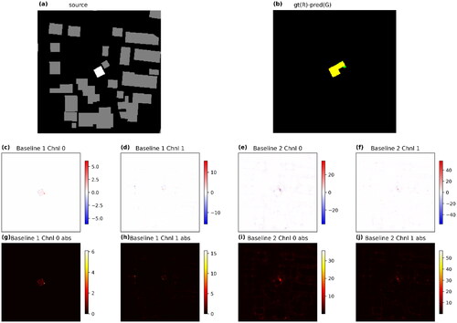
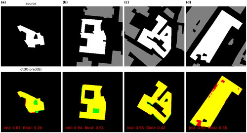
Figure 3 shows a sample result of a focal building whose ground truth of map generalization is the result of aggregation with two nearby buildings and further simplification of the aggregated polygon. The prediction by the deep neural network is quite reasonable; there are only a few sets of mistakenly predicted pixels (green and red pixels in Figure 3(b)). The output of Baseline 1, Channel 0 (Figure 3(c,g)) reveals that the DL neural network focuses on the boundary pixels of the focal building, but the interior pixels are also noticed, though their values are much closer to zero but not totally zero. Along the boundary pixels of the focal building, the DL neural network also has a higher focus on the corners and the edge of the protrusion at the bottom, which is removed as a matter of simplification.

Figure 3. IG results of a test sample. (a) The white polygon is the focal building to be generalized. The gray polygons are its surrounding buildings. (b) The ground truth of the generalized building is in the red channel. The DL-predicted building is in the green channel. Thus, the yellow pixels show the true positives. (c) and (d) Raw IG values with Baseline 1. Color ramp is normalized to let the white color correspond to 0. (e) and (f) Raw IG values of Baseline 2. (g) and (h) Absolute values of IG values with Baseline 1. (i) and (j) Absolute values of IG values with Baseline 2.

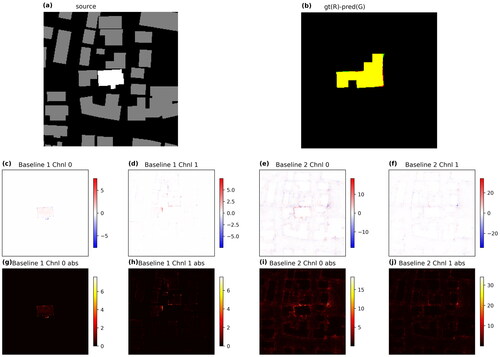
It can also be observed that the boundaries of surrounding buildings contained in Channel 1, especially the two that are combined with the focal building, also contribute much more to the prediction than the corresponding interior (Figure 3(d,h)). The results of Baseline 2 (Figure 3(e,f,i,j)) show more explicitly that the DNN checks information in both channels in an integrated manner, as the integrated gradients of both channels show the profile of all buildings. The pixels near the focal building have higher absolute values, which is reminiscent of the First Law of Geography in that the DNN pays more attention to the nearby region of the focal building. More examples (Appendix Figures A1–A3) give a similar impression as the aforementioned sample result, regardless of the quality of the prediction.

The results of the layer activation are shown in Figure 4. Most activation patterns of the Conv1 convolution block are similar to the raw input, as expected. However, it is easy to tell that the overall spatial layout has been decomposed: Some dimensions have a focus on the focal building as a whole (Channels 3-c, 5-d, 5-e, and 7-a), some dimensions respond to the boundary of the focal building (Channels 1-d, 6-g, and 8-c), or the boundaries of the surrounding buildings (Channel 7-c), similar to the observations made from the results of IG. The space surrounding the buildings is noticed as a whole (Channels 1-b and 7-d), while the space between the focal building and the two buildings that it is aggregated with receives more attention (Channel 4-b (as enlarged in Figure 5(a)). 4-d (as enlarged in Figures 5(b), 4-g, and 5-h). Channels 4-c, 6-c, and 7-d show that aggregating the three buildings into one is already an option for the neural network’s output.

Figure 4. Layer activation of Conv1 convolution block in the trained ResU-Net with the same input as in Figure 3. Numbers and letters are for reference purposes only. They are not related to their actual sequence in the layer.

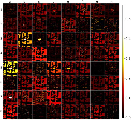
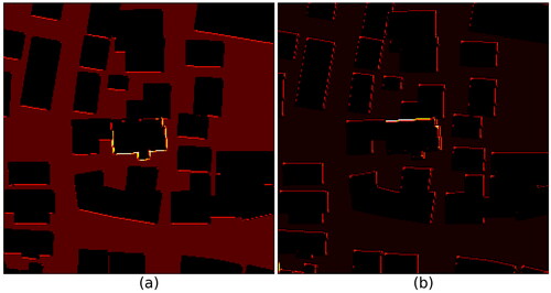
Figure 5. Enlarged layer activation of Conv1 convolution blocks (a) 4-b as in Figure 4. (b) 4-d as in Figure 4.

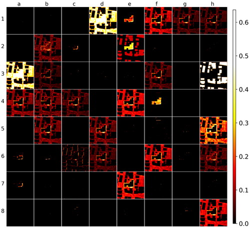
The activation patterns of the final up-sampling layer (Figure 6) give hints as to how the final output is composed. Channels 1-e and 4-f solely show the shape of the output. The removed protrusion as aforementioned is paid attention by the network (Channels 1-g, 3-f, 4-a, 6-d, etc.). We can also notice that some channels are more focused on the single building parts, such as Channels 2-c, 6-a, 6-b, 7-a, etc. Other channels take the spatial layout of the whole region into account, such as Channels 1-d, 1-f, 3-a, 4-e, etc.

Figure 6. Layer activation of UpConv1 convolution block in the trained ResU-Net with the same input as in Figure 3. Numbers and letters are for reference purposes only. They are not related to their actual sequence in the layer and have no correspondence relationship to those in Figure 4.

In general, the DNN would like to check the spatial relationship of the buildings, as evidenced by the higher absolute IG values of the pixels in the space between the buildings and the visualization of the layer activation. For modification of the building shape, the edges and corners near the desired parts are more important to the DNN.

5.2. Quantitative analysis of results of IG with Baseline 1

The absolute values of IG with Baseline 1 have high skewness for the whole image and for its boundary and interior pixels, respectively, as the example of Figure 7 shows. Therefore, using the non-parametric mean test (Mann-Whitney U test) is a reasonable choice. Applied to 100 randomly selected map patches, the Mann-Whitney U test is significant for an overwhelming number of cases (95 out of 100), meaning that their mean is significantly larger for their absolute values of IG at the boundary than in the interior (Table 1). For the five samples whose boundary and interior show similar influence on the final outputs, we observe that they are all trivial cases for the U-Net: In each of these map patches, there is no change between the initial building and its generalized version, and the prediction is almost perfect. We can further observe that their ranges of absolute IG values are also much smaller than in other cases (Figure 8).

Figure 7. Histograms of the IG absolute values of the test sample in Figure 3 by boundary and interior pixels.

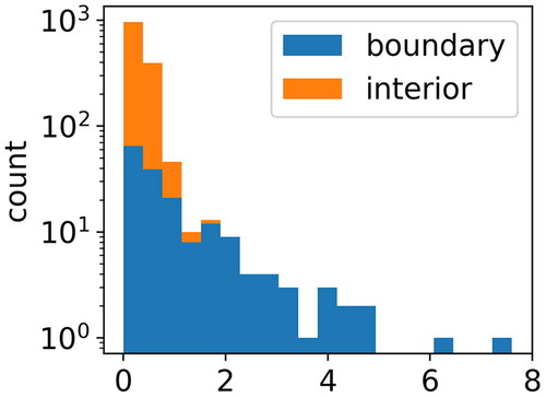
Figure 8. The five samples with p-value larger than 0.05 in Table 1.

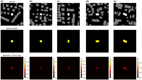
Table 1. Number of samples with corresponding p-value in the Mann-Whitney U tests.

N = 100	p-value
89	***
4	**
2	*
5	–

*** :p-value < 0.001; **:p-value [0.001, 0.01]; *:p-value [0.01, 0.05]: -: p-value >0.05.

5.3. BIoU as an evaluation metric for the existing test result

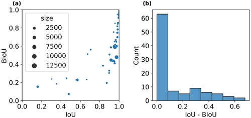
The comparison between BIoU and IoU clearly shows that BIoU has a different focus from the IoU, as the BIoU values of the sample set are smaller than the corresponding IoU values (Figure 9). The difference between BIoU and IoU seems not to be related to the size of the buildings, as we observe that the points deviating farthest from the diagonal of Figure 9(a) do not necessarily have the largest sizes. As Figure 9(b) further suggests, the differences are not always big, as the majority clusters in the range between 0 and 0.1. However, roughly half of the cases have much larger differences, which suggests that the BIoU as a performance metric can be more sensitive to certain cases.

Figure 9. (a) IoU and BIoU values of the 100 test samples. Size is defined as the number of pixels of the original building. (b) Difference between IoU and BIoU for the test samples.

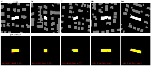
A closer investigation of some sample patches suggests what kinds of scenarios the BIoU can be sensitive to. The predictions in Figure 10 are all visually close to their ground truth. There is a very small proportion of difference as marked in red and green, which places the defects on the edges of the polygon. It is even more obvious in Figure 10(a) that the desired generalized building should be L-shape while the prediction is closer to a rectangle. However, such a small difference leads to a very big difference between their IoU and BIoU values, no matter if the difference distributes along the boundary, e.g. Figure 10(b,d,e), or the difference clusters, e.g. Figure 10(c).

Figure 10. The top five samples with the largest difference between their IoU and BIoU values. Color scheme for channels is the same as Figure 3.

Samples in the test set do not contain buildings with holes, as the test site is a suburban area of Stuttgart, while the training and validation sets cover the downtown area. We examined 31 building samples in the validation set and found that BIoU is more sensitive to the holes than IoU as well (Figure 11). Selected samples (Figure 12(a,c)) show that even if a hole is mistakenly filled by the DNN, the IoU values are still relatively high, if the hole is not big. However, for BIoU, the same samples will receive a low value. We can also see from Figure 12(b–d) that if the hole is big enough, the DNN can certainly maintain the hole and tries to make the correct generalization. Figure 12(c,d) also show that even if the hole is small, it is not necessary that the DNN would fill it in, meaning some spatial context regarding the hole is learned. Therefore, BIoU can also serve as a metric for evaluating map generalization results, especially for defects along the edges and corners.

Figure 11. (a) IoU and BIoU values of the 31 samples from validation set. Size is defined as the number of pixels of the original building. (b) Difference between IoU and BIoU for the test samples.

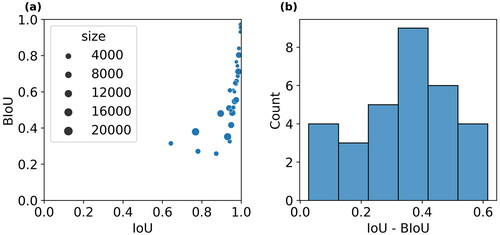
Figure 12. Selected building-with-hole samples with large differences between their IoU and BIoU values. Color schema for channels is the same as Figure 3.

6. Discussion

This study utilizes XAI tools, particularly integrated gradients and layer activation, to explore if a DL neural network trained to generalize buildings has learned cartographic knowledge that human beings possess. In the visual analytics on the results of IG with Baseline 1, we observe that the hotspots appear at the boundary rather than the interior parts. The results of statistical tests further confirm the hypothesis that the boundaries of the buildings are more important than the interior parts of the buildings for the U-Net to predict the output (Section 5.2). That fits the human drawing process, where we typically delineate the boundary of a geometric shape first and then fill the interior. The visual analytics on the results of IG with Baseline 2 suggest that the deep neural network not only checks the boundary of the focal building it generalizes but also the boundaries of certain surrounding buildings and the space between the focal building and selective surrounding buildings, particularly those who are candidates for aggregation. Visual inspection of the layer activation also shows patterns similar to the results of IG. The network builds ideas of building parts, aggregation, and surrounding areas. It should be noted that such focus is not evenly distributed among the buildings nor the space, indicating that the DL neural network takes the spatial layout of the buildings into account but prioritizes their importance accordingly before making a decision. This fits the contextual generalization process of cartographic knowledge where the generalization of individual objects is dependent on its environments (Ruas and Duchêne 2007). Thus, we can answer the research question at least partially that the DNN we used in this study has learned some human-interpretable cartographic knowledge, simplification and aggregation operators in particular, when it is applied to map generalization tasks.

We further examined the performance of Boundary IoU as an evaluation metric for raster-based map generalization. As the results of the 100 test samples show, BIoU is very sensitive to errors along the exterior and interior boundaries compared to IoU. Overall, that finding matches our expectations. We recommend that researchers use BIoU for the evaluation of similar studies in the future, which can further depict the fine-grained performance in predicting object shapes. In addition to being an evaluation metric, BIoU might also be helpful as part of an integrated loss function in DL-based map generalization, as it is used in other GeoAI applications, such as remote sensing (Yang et al. 2023), as it emphasizes the importance of precise matching at the boundary.

There are a few limitations of this study. The integrated gradients method provides a pairwise connection between the two pixels at the same location in the input and output. However, the method cannot provide insights into the spatial dependency of the neighborhood given a certain pixel. That is to say, given a focal pixel, we do not know to which extent each of the nearby pixels influences the decision-making of the DNN. Therefore, we are not able to tell what high-level structures as combinations of pixels may correspond to certain output patterns. Given the example of the protrusion at the bottom of the focal building in the source map of Figure 3, we notice that the DNN removes the protrusion as a matter of simplification, and the decision is related to the nearby pixels, implying that some structural influence was likely applied. However, it cannot be inferred that such a decision is related to preserving the overall area, which is a common principle in polygon-based map generalization. To summarize, the integrated gradient method only accounts for pixel-to-pixel relationships, which does not offer insights into whether the neural network has learned local or regional spatial structures of those buildings. Our analytical method with semantic segmentation based on pixels partially moderates the shortcomings of attributing gradients, which is regarded as one of the challenges in applying XAI to GeoAI (Xing and Sieber 2023). However, cartographic map generalization involves more attributes, such as direction, distance, and spatial dependency, which make it unique and distinguish it from ordinary computer vision tasks. New XAI methods need to be developed for further insights.

7. Conclusions

This study proposes an XAI-supported workflow to reason about the cartographic knowledge learned by a deep neural network that was trained for map generalization tasks on buildings. With qualitative and quantitative analytical tools, we demonstrate that a DNN can learn human-interpretable cartographic knowledge. Particularly, we find that the boundaries of buildings influence the decision-making process of a DNN more than the interior parts of the buildings. Such an observation can help us improve the performance of model training by introducing new items, such as the Boundary IoU, into the loss function. Overall, the study shows that XAI can help reveal scientific insights for DL-based map generalization. Our future work will explore how building parts, such as the location of protrusions and the spatial layout of the buildings, may influence the operations that the deep learning networks apply to the focal building.

Acknowledgments

The authors would like to thank Dr. Yu Feng at the Technical University of Munich for sharing the raw building maps of Stuttgart, Germany.

Disclosure statement

No potential conflict of interest was reported by the author(s).

Data and codes availability statement

The data and code that support the findings of this study are available in ‘figshare.com’ with the identifier https://doi.org/10.6084/m9.figshare.24948057.v1.

Additional information

Funding

This work has received funding from the Swiss National Science Foundation under project number 200021_204081, project DeepGeneralization.

Notes on contributors

Cheng Fu

Cheng Fu is a Lecturer in the Department of Geography, University of Zurich, Switzerland. His research interests are place modeling, human mobility, and map generalization. He contributed to conceptualization, methodology, software development, validation, formal analysis, data curation, writing, reviewing, editing, and visualization.

Zhiyong Zhou

Zhiyong Zhou is a postdoctoral researcher in the Department of Geography, University of Zurich, Switzerland. His research interests include location based services (LBS), computational cartography, spatial data science, and urban analytics. He contributed to conceptualization, methodology, formal analysis, data curation, reviewing, editing and visualization.

Yanan Xin

Yanan Xin is a Senior Research Assistant at the Mobility Information Engineering Lab, Institute of Cartography and Geoinformation, ETH Zurich. Her research interests are computational mobility analysis, mobility-based anomaly detection, interpretable machine learning, and spatial causal inference. She contributed to conceptualization, methodology, writing review and editing.

Robert Weibel

Robert Weibel is a Professor of Geographic Information Science at the University of Zurich, Switzerland. He is interested in mobility analytics with applications in transportation and health, spatial analysis for linguistic applications, and computational cartography. He contributed to supervision, investigation, formal analysis, reviewing, editing, and project administration.

Appendix A

Figure A1. Additional sample of IG results. Annotations are the same as Figure 3 in the main text.

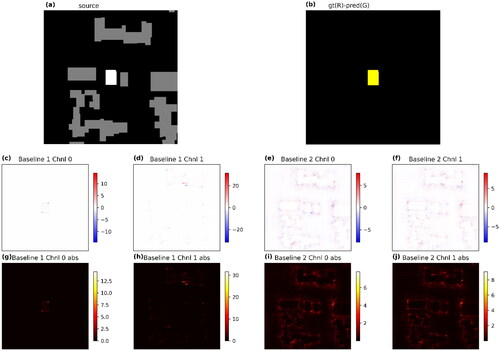
Figure A2. Additional sample of IG results. Annotations are the same as Figure 3 in the main text.

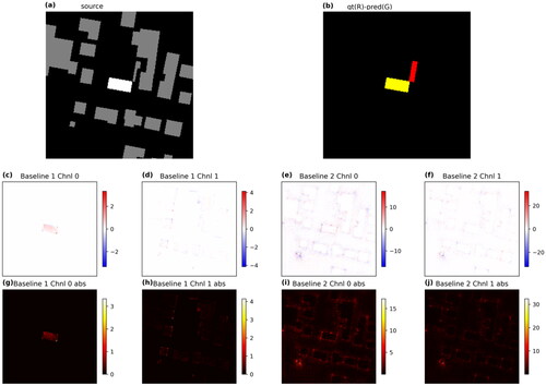
Figure A3. Additional sample of IG results. Annotations are the same as Figure 3 in the main text.

References

- Arrieta, A.B., et al., 2020. Explainable Artificial Intelligence (XAI): concepts, taxonomies, opportunities and challenges toward responsible AI. Information Fusion, 58, 82–115.
- Bader, M., Barrault, M., and Weibel, R., 2005. Building displacement over a ductile truss. International Journal of Geographical Information Science, 19 (8-9), 915–936.
- Barrault, M., et al., 2001. Integrating multi-agent, object-oriented and algorithmic techniques for improved automated map generalization. Proceedings 20th International Cartographic Conference, 1, 2110–2116.
- Beard, K., 1991. Constraints on rule formation. In: Map Generalization: Making Rules for Knowledge Representation. London, England: Addison-Wesley Longman Ltd., 121–135.
- Bokhovkin, A., and Burnaev, E., 2019. Boundary loss for remote sensing imagery semantic segmentation. Lecture Notes in Computer Science (Including Subseries Lecture Notes in Artificial Intelligence and Lecture Notes in Bioinformatics), 11555 LNCS (14), 388–401.
- Bradski, G., 2000. The openCV library. Dr. Dobb’s Journal: Software Tools for the Professional Programmer, 25 (11), 120–123.
- Brassel, K.E., and Weibel, R., 1988. A review and conceptual framework of automated map generalization. International Journal of Geographical Information Systems, 2 (3), 229–244.
- Burghardt, D., Duchêne, C., and Mackaness, W. (Eds.). 2014. Abstracting Geographic Information in a Data Rich World: Methodologies and Applications of Map Generalisation. Cham Switzerland: Springer International Publishing.
- Cheng, B., et al., 2021. Boundary IoU: improving object-centric image segmentation evaluation. In: 2021 IEEE/CVF Conference on Computer Vision and Pattern Recognition (CVPR), Nashville, Tennessee, 15329–15337.
- Courtial, A., Touya, G., and Zhang, X., 2022. Representing vector geographic information as a tensor for deep learning based map generalisation. AGILE: GIScience Series, 3, 1–8.
- Courtial, A., Touya, G., and Zhang, X., 2023. Deriving map images of generalised mountain roads with generative adversarial networks. International Journal of Geographical Information Science, 37 (3), 499–528.
- Courtial, A., Touya, G., and Zhang, X., 2024. DeepMapScaler: a workflow of deep neural networks for the generation of generalised maps. Cartography and Geographic Information Science, 51 (1), 41–59.
- Du, J., et al., 2022. Polyline simplification based on the artificial neural network with constraints of generalization knowledge. Cartography and Geographic Information Science, 49 (4), 313–337.
- Feng, Y., Thiemann, F., and Sester, M., 2019. Learning cartographic building generalization with deep convolutional neural networks. ISPRS International Journal of Geo-Information, 8 (6), 258.
- Fu, C., et al., 2023. Keeping walls straight: data model and training set size matter for deep learning in building generalization. Cartography and Geographic Information Science, 51 (1), 1–16.
- Gao, Y., et al., 2024. Going beyond XAI: a systematic survey for explanation-guided learning. ACM Computing Surveys, 56 (7), 1–39.
- Harrie, L.E., 1999. The constraint method for solving spatial conflicts in cartographic generalization. Cartography and Geographic Information Science, 26 (1), 55–69.
- Harrie, L., et al., 2024. Machine learning in cartography. Cartography and Geographic Information Science, 51 (1), 1–19.
- Hasanpour Zaryabi, E., et al., 2022. Unboxing the black box of attention mechanisms in remote sensing big data using XAI. Remote Sensing, 14 (24), 6254.
- Hsu, C.-Y., and Li, W., 2023. Explainable GeoAI: can saliency maps help interpret artificial intelligence’s learning process? an empirical study on natural feature detection. International Journal of Geographical Information Science, 37 (5), 963–987.
- Hu, Y., et al., 2024. A five-year milestone: reflections on advances and limitations in GeoAI research. Annals of GIS, 30 (1), 1–14.
- Janowicz, K., et al., 2020. GeoAI: spatially explicit artificial intelligence techniques for geographic knowledge discovery and beyond. International Journal of Geographical Information Science, 34 (4), 625–636.
- Janowicz, K., et al., 2022. Six GIScience ideas that must die. AGILE: GIScience Series, 3, 1–8.
- Kang, Y., Gao, S., and Roth, R.E., 2024. Artificial intelligence studies in cartography: a review and synthesis of methods, applications, and ethics. Cartography and Geographic Information Science, 1–32.
- Kang, Y., et al., 2020. Towards cartographic knowledge encoding with deep learning: a case study of building generalization. The 23rd International Research Symposium on Cartography and GIScience, 2019, 1–6.
- Kervadec, H., et al., 2021. Boundary loss for highly unbalanced segmentation. Medical Image Analysis, 67, 101851.
- Kipf, T.N., and Welling, M., 2019. Semi-supervised classification with graph convolutional networks. In: 5th International Conference on Learning Representations, ICLR 2017 - Conference Track Proceedings, Toulon, France, 1–14.
- Kokhlikyan, N., et al., 2020. Captum: A unified and generic model interpretability library for PyTorch. (arXiv:2009.07896), arXiv.
- Larochelle, H., et al., 2009. Exploring Strategies for Training Deep Neural Networks. Journal of Machine Learning Research, 1, 1–40.
- LeCun, Y., Bengio, Y., and Hinton, G., 2015. Deep learning. Nature, 521 (7553), 436–444.
- Li, J., et al., 2023. Interpreting deep learning models for traffic forecast: a case study of unet. SSRN Electronic Journal.
- Mackaness, W.A., Ruas, A., and Sarjakoski, L.T., 2007. Generalisation of geographic information: Cartographic modelling and applications. Amsterdam, Netherlands: Elsevier.
- Mai, G., et al., 2022. Towards general-purpose representation learning of polygonal geometries. GeoInformatica, 27 (2), 289–340.
- Müller, J.-C., et al., 1995. Generalization: State of the art and issues. In: J.-C. Müller, J. P. Lagrange, & R. Weibel, eds. GIS And Generalisation: Methodology and Practice. Oxfordshire, UK: Taylor & Francis.
- Powitz, B.M., 1993. Computer-assisted generalization-an important software tool in GIS. International Archives of Photogrammetry and Remote Sensing, 29, 664–672.
- Ruas, A., and Duchêne, C.A., 2007. A prototype generalisation system based on the multi-agent system paradigm. In: Generalisation of Geographic Information. Amsterdam, Netherlands: Elsevier.
- Saeidi, V., et al., 2023. Water depth estimation from Sentinel-2 imagery using advanced machine learning methods and explainable artificial intelligence. Geomatics, Natural Hazards and Risk, 14 (1), 2225691.
- Sester, M., 2005. Optimization approaches for generalization and data abstraction. International Journal of Geographical Information Science, 19 (8-9), 871–897.
- Shi, M., et al., 2023. Thinking geographically about AI sustainability. AGILE: GIScience Series, 4, 1–7.
- Shrikumar, A., Greenside, P., and Kundaje, A., 2017. Learning important features through propagating activation differences. In: Proceedings of the 34 Th International Conference on Machine Learning. https://proceedings.mlr.press/v70/sundararajan17a.html
- Simonyan, K., Vedaldi, A., and Zisserman, A., 2014. Deep inside convolutional networks: visualising image classification models and saliency maps. (arXiv:1312.6034). arXiv. http://arxiv.org/abs/1312.6034
- Sundararajan, M., Taly, A., and Yan, Q., 2017. Axiomatic attribution for deep networks. In: Proceedings of the 34 Th international conference on machine learning. http://arxiv.org/abs/1703.01365
- Swiss Society of Cartography 2005. Topographic Maps: Map Graphics and Generalisation (Issue Issue 17 of Cartographic publication series).
- van der Velden, B.H.M., et al., 2022. Explainable artificial intelligence (XAI) in deep learning-based medical image analysis. Medical Image Analysis, 79, 102470.
- Weibel, R., and Dutton, G., 1998. Constraint-based automated map generalization. In: Proceedings 8th International Symposium on Spatial Data Handling, Lisbon, Portugal, 214–224.
- Weibel, R., and Dutton, G., 1999. Generalising spatial data and dealing with multiple representations. Geographical Information Systems, 1, 125–155.
- Weibel, R., Keller, S., and Reichenbacher, T., 1995. Overcoming the knowledge acquisition bottleneck in map generalization: The role of interactive systems and computational intelligence. Lecture Notes in Computer Science (Including Subseries Lecture Notes in Artificial Intelligence and Lecture Notes in Bioinformatics), 988, 139–156.
- Wilson, I.D., Ware, J.M., and Ware, J.A., 2003. A Genetic algorithm approach to cartographic map generalisation. Computers in Industry, 52 (3), 291–304.
- Xiao, T., et al., 2023. A point selection method in map generalization using graph convolutional network model. Cartography and Geographic Information Science, 51 (1), 20–40.
- Xing, J., and Sieber, R., 2021. Integrating XAI and GeoAI. GIScience 2021 Short Paper Proceedings. In: 11th International Conference on Geographic Information Science. September 27-30, Poznań, Poland (Online).
- Xing, J., and Sieber, R., 2023. The challenges of integrating explainable artificial intelligence into GeoAI. Transactions in GIS, 27 (3), 626–645.
- Yan, X., et al., 2020. Graph convolutional autoencoder model for the shape coding and cognition of buildings in maps. International Journal of Geographical Information Science, 35 (3), 490–512.
- Yan, X., et al., 2022. A graph deep learning approach for urban building grouping. Geocarto International, 37 (10), 2944–2966.
- Yang, J., Matsushita, B., and Zhang, H., 2023. Improving building rooftop segmentation accuracy through the optimization of UNet basic elements and image foreground-background balance. ISPRS Journal of Photogrammetry and Remote Sensing, 201, 123–137.
- Yu, W., and Chen, Y., 2022. Data‐driven polyline simplification using a stacked autoencoder‐based deep neural network. Transactions in GIS, 26 (5), 2302–2325. https://doi.org/10.1111/tgis.12965
- Zhang, Z., Liu, Q., and Wang, Y., 2018. Road extraction by deep residual U-net. IEEE Geoscience and Remote Sensing Letters, 15 (5), 749–753.
- Zheng, J., et al., 2021. Deep graph convolutional networks for accurate automatic road network selection. ISPRS International Journal of Geo-Information, 10 (11), 768.
- Zhou, Z., Fu, C., and Weibel, R., 2022. Building simplification of vector maps using graph convolutional neural networks. Abstracts of the Ica, 5, 1–2.
- Zhou, Z., Fu, C., and Weibel, R., 2023. Move and remove: Multi-task learning for building simplification in vector maps with a graph convolutional neural network. ISPRS Journal of Photogrammetry and Remote Sensing, 202, 205–218.