Evolving model architecture for custom output range exploration

Abstract

In this paper, a methodology for combined online design of experiments and system identification is presented. More specifically, the paper addresses the problem of creating a model automatically that describes an unknown process accurately in a predefined range of its output. Such a model is typically needed for the calibration of combustion engines where only a relatively small emission range is of interest. The presented solution approach consists of two interacting components: first, an evolving local model network is used for creating, refining and extending a data-driven model, based on the incoming measurements; second, model-based approaches are proposed for designing new experiments so that the data-driven model has a high degree of accuracy in a predefined range of its output. The method uses, besides the models, a space-filling to explore untrained areas. The proposed concepts are illustrated and discussed by means of an academic and two real-world examples.

Keywords:

• online design of experiments
• online training
• non-linear system identification
• local model networks

1. Introduction

Data-driven models and experiment design are tools that are vastly used in very different domains in order to gain insight into complex and non-linear processes. Applications range from the identification of the processes to their calibration.

The required quality of data-driven models strongly depends on their intended purpose which covers fields as different as prediction, classification, diagnosis, optimization or control. Many application fields require the accuracy of a model to be high only in a limited range of its inputs. Such a range is typically prescribed by the operational limits of the underlying process or by economic or legal constraints. Typical examples are combustion engines that are operated to achieve high performance with reduced environmental impact by complying with mechanical constraints; the feasible ranges of process inputs like the engine speed or the intake manifold pressure are fixed by the engine design and determined by expertise.

On the other hand, the operation of many processes is governed or limited by one or more of their outputs. A typical example in this context is emissions created during the operation of combustion engines or power plants. Especially the operation of power plants is often only economically viable closely to legal emission limits. Also, one might consider the large class of processes that are critically limited by constraints on their outputs or internal states. Pasteurization plants serve as an example from the process industry where the so-called pasteurization temperature has to be kept within tight limits. Another example is given by engine exhaust temperature which is limited from below by catalyst effectiveness and from above due to material constraints. Thus, a model is only relevant within these limits, regardless of its inputs.

The problem of automatically obtaining a data-driven model that is accurate within a predefined output range is challenging in that knowledge of the actual output can generally only be obtained from the data-driven model itself so that in principle an interaction problem is posed; designing the proper experiments to produce a data-driven model that is accurate in a certain region of the output requires quantitative knowledge of the unknown input/output relation to be modelled, and vice versa.

The problem of data-driven modelling in a custom output range is addressed in the literature through output constraints. [1] designs experiments to maintain the actual output to a feasible range using a constrained optimization based on the model estimation. Other methods may estimate the level sets corresponding to both the upper and the lower value of the custom output range, which allows to transforms output constraints into input constraints, but which also poses the level set estimation problem [2–4]; present methodologies that adaptively generate experiments targeting directly the level set estimation. [5] tackles the level set estimation indirectly using an infinitely narrow region around a custom output using fuzzy boundaries. From the previously cited methods, the method of this paper differs: it does not targets a level set estimation, but targets a model parameterization in a custom output range, which is presumed large; it does not simply constrain the output to the custom output range, but also considers the data distribution in that custom output range to design new experiments.

1.1. Solution approach

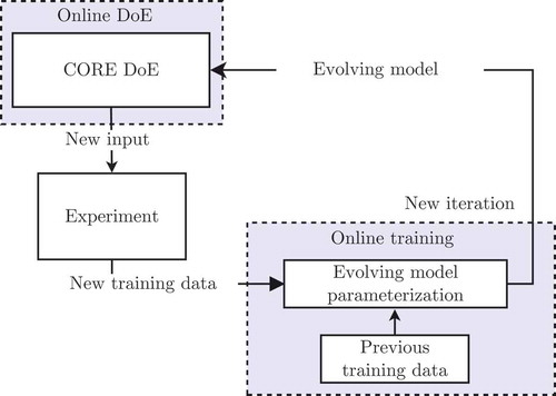
In this paper, a new and integrated concept for experiment design and data-driven modelling is proposed that manages to produce models that accurately resemble an unknown process in a custom output range (). The novelty of the approach lies in the way new experiments are scheduled: while pre-existing concepts are based on a certain model structure and a data distribution in the input space of the model (see [6]), the proposed concept explicitly considers data distribution also in the output space. It constitutes an iterative procedure where at each iteration step a data-driven model is used to predict the process output and to explore unknown regions of the input/output space. The iteration process starts with an initial design of experiments (DoE) which is used to parameterize an initial model. Both the DoE and the data-driven model are subsequently extended in such a way that relevant domains of the design space are explored. This process is termed custom output range exploration (CORE).

The CORE relies on an automatic adaptation technique and evolving scheme for data-driven models (see [7]), which is known as online training. The online trained data-driven models to outline the input/output relation increasingly well, when the training data set grows. Data-driven models that update their structures and parameters with the acquisition of new training data are known as evolving models. The CORE uses an evolving model to produce new experiments online (see Figure 1), which is known as online DoE (see [1]).

Figure 1. Interaction between online DoE and online training for CORE.

In the literature, multiple model architectures are used for online DoE. The model architecture to be chosen must comply with the properties of the process to be modelled. The considered processes can be non-linear time-invariant or time-variant processes. The local model networks (LMNs) present suitable model architecture to handle those kinds of processes (see [8]). In contrary to other model architectures like the multi-layer perceptrons, the retained training of the LMNs is done without parameters that depend on a random initialization that can lead to a poor training of the models (see [9]). The training reliability is decisive for the CORE, since the quality of the online DoE depends directly on the quality of the evolving model. [10] shows the quality increase procured by an online DoE that is carried out with LMNs, which are refined by increasing the number of local models iteratively, compared to a conventional method for the model parameterization. In this paper, the evolving models for the CORE are evolving LMNs (ELMNs) (see [11]). The advantage of the ELMNs, compared to LMNs parameterized with batch training, is that they adapt automatically to new online observations by resuming the model parameterization, according to a structure criterion for determining the number of local models. The ELMNs therefore offers a convenient class of model for the online training.

Besides the online training, the CORE DoE relies on an online DoE that is conceived for the process exploration in a custom output range. The proposed CORE DoE is an extension of the state-of-the-art maximin distance design (MDD) (see [12]), which serves for process exploration of inputs values in predefined input ranges. MDD relies on topological (geometrical) principles, which basic idea consists in representing experiments using design points. The coordinates of a design point are the q input values that are applied to the process during an experiment. The design points are thus distributed in a q-dimensional design space, which is a bounded subset of . Considering a distance for the metric input space, e.g. the popular Euclidean distance, [13] uses MDD for distributing design points uniformly in complex design spaces. The proposed CORE DoE differs from that MDD exploration in that the metric space considered for the distance calculation is not only limited to the input space, but is also extended to the output space. Moreover, the CORE DoE is not conceived to generate an optimal design for a given number of design points, but constitutes a procedure for an iterative design point selection. Three variants of the CORE DoE are proposed in this paper, which differ by the considered distances for the design point selection. The three distances are Euclidean distances to be distinguished by the metric spaces to which they are associated: the input space, the output space and the input/output space that is the Cartesian product of both input and output space.

The remainder of this paper is structured as follows: Section 2 describes the ELMN architecture and training procedure. Section 3 describes the CORE DoE and presents the reasons for which attention is placed on the comparison of three distances associated to the input, the output and the input/output space. In Section 4, the proposed approaches are exposed by mean of an illustrative example to highlight the advantages and limitations of the method in this paper. Section 5 describes the results achieved after application of the method to Diesel engines in order to estimate and soot emissions in . Finally, Section 6 presents the conclusions that are drawn from the presented results.

2. Evolving local model network architecture

The online training of evolving models requires adjusting, refining, extending and evolving an already trained model with new data (see [7]). Consequently, an update of the model parameters during the operation of the system is necessary. Since it is not possible to completely rebuild the model using all measurement data in each step, the model is evolved iteratively and therefore its complexity augments gradually.

The proposed concepts for CORE are presented with the ELMN described in ref. [11], but other model architectures can be used as well, on condition that they are able to predict the system output suitably. In this section, that ELMN training algorithm is shortly reviewed.

LMNs interpolate between local models, which can easily be described using linear regression models, i.e. a linear combination between m parameters and predictor variables, potentially non-linearly transformed and collected in a regressor vector . The non-linear system is approximated by partitioning those regions of the input/output space, where the non-linearity is more complex, into smaller subdomains. Each local model – indicated by subscript i – consists of two parts: its parameter vector and its validity function .

The validity function defines the region of validity of each local model. An important topic in non-linear system identification is the incorporation of prior knowledge. In this context, one of the main strengths of LMNs is that the premises (i.e. the validity functions) and the consequents (i.e. the local model outputs) do not necessarily depend on identical variables (i.e. and , respectively) (see [14]). Thus, the partition space, which is spanned by the premise vector , is chosen in advance to describe the validity of the local models.

The regressor vector contains past system inputs and outputs in case of dynamic system identification. In case of static modelling, the local models are typically represented by polynomial regression models where the relationship between the inputs and the output is modelled as an nth order polynomial. In this paper, the considered processes are time-invariant processes that are efficiently modelled using quadratic polynomials including interaction terms, which are collected in the regressor vector :

(1)

The local estimates are computed from a scalar product of the regressor vector and the parameter vectors :

(2)

All local estimates are used to form the global model output by weighted aggregation:

(3)

where M is the number of local models. Note that the ELMN parameters and predictor variables do not form a linear combination. The non-linearity is due to the non-linear behaviour of the validity functions which take, e.g. values between 0 and 1 according to the premise vector . Figure 2 shows how the non-linear validity functions (see lower axes) act on the quadratic polynomials to produce a global output close to the training data of an unknown process (see upper axes).

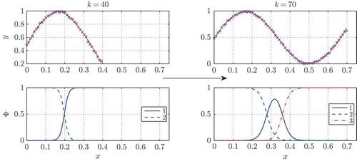
Figure 2. ELMN approximating an unknown process. Upper axes: model output (red line) is compared to training data (blue crosses). Lower axes: validity functions of local models are depicted. On the left: ELMN with two local models. On the right: ELMN with three local models.

The computation of the validity functions is based on a binary discriminant tree where each node corresponds to a split of the partition space into two parts (see [15]). The free ends of the branches represent the actual local models with their validity functions and their parameter vectors and the nodes represent weight vectors of the partitions (see Figure 3). In this paper, the binary discriminant tree is a logistic discriminant tree; the nodes split the partition space using logistic sigmoid activation functions with multiple explanatory variables.

Figure 3. Logistic discriminant trees of ELMNs with two and three local models.

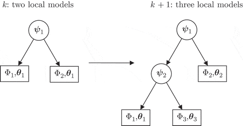
The main challenge with the training of evolving models is to build the model incrementally whenever new data are available. The decomposition of the partition space of the proposed ELMN is performed recursively. This incremental model construction allows the complexity of the ELMN to increase gradually: when the number of local models M is incremented by one, the worst local model (indexed by l) of the logistic discriminant tree (Figure 3) is replaced by a new node and two adjoining local models are appended. On the one hand, this strategy allows a proper initialization of the new model parameters while on the other hand the computational demand is low.

The weight vector and the parameters of the new local models are obtained using a recursive non-linear least squares algorithm. In order to reduce the computational demand, only the weight vector of the actual node and the parameters and are optimized with a non-linear least square algorithm. Since the validity functions (i.e. the weight vectors ) of the remaining local models are not modified during the split optimization, the remaining parameters are updated using the conventional weighted least squares method.

The incremental model construction is repeated until an optimal number of local models is reached according to a structure criterion which determines a reasonable complexity for the ELMN, for a given amount of training data. The chosen structure criterion is a splitting rule for the determination of the optimal number of local models. The spilling rule is based on the assumption that the residual distribution of each local linear model follows a chi-squared distribution and is calculated as described in ref. [11].

3. Custom output range exploration methodology

3.1. Design point selection and candidate set

The proposed DoE approach for non-linear systems is motivated by applications for which high model accuracy is required in a very specific range of the process output, which is defined by a minimal output value and a maximal output value . The custom output range is assumed to be known (e.g. feasible emission range of an engine):

(4)

The set of the applied design points

(5)

and the set of the observed process outputs

(6)

are growing until an ELMN with high quality in is trained.

The proposed DoE approach requires an initial design consisting of design points. The initial design is used for producing training data which can be random (see previous training data in Figure 1) (see [16]). The initial number of design points and the design point distribution are chosen in such a way that the model parameter covariance matrix is not singular. An ELMN is trained with its most simple structure (with a single local model) using the initial training data and a weighted least squares algorithm. Using the ELMN, the proposed DoE approach produces iteratively design points. The number of data required for fitting the process output depends on the design point distribution, the model structure and the noise level (see [17]).

The proposed CORE DoE targets the generation of design points corresponding to process outputs within during the experiment. The intended purpose is to produce training data in , so that the quality of the ELMN iteratively increases in . In order to simplify the problematic, the CORE DoE strategy selects with every iteration (indexed by ) a design point from a predefined candidate set of design points instead from the whole design space. That initial candidate set consists of a fixed number N of design points and is denoted by . Reducing the design space to the candidate set is a strong restriction for the design point selection. That restriction is attenuated by generating the initial candidate set with a high number of design points covering uniformly all the feasible input ranges.

The proposed CORE DoE targets a strict exploration of the design space, which means that repetition points are avoided. Thus, the set of remaining design points in to be applied to the system decreases in every iteration k. For reasons of convenience, that remaining candidate set of design points is denoted , which is to be distinguished from the initial candidate design set . In concrete terms, in every iteration k a new design point from is applied to the system, the output is observed and the ELMN is updated (see Equation (3)), as depicted in Figure 1.

The selection of the design points in is based on a two-step strategy. First, in each iteration k, a reduced candidate set, denoted , is generated from the design points in and from the ELMN, by selecting the design points with a model output in . Second, a selection criterion is applied to for determining the applied design points that iteratively produce training data parameterizing the ELMN in .

The following subsection presents how the reduced candidate set is generated from the remaining candidate set and which properties the initial candidate set must have for a proper generation.

3.2. Generation of the candidate set in

The candidate set is a fixed finite set of design points that is required to uniformly cover the feasible range of the q-dimensional design space. For the generation of , a state-of-the-art full factorial design is chosen, which consists of q factors each with p levels. A full factorial design is used because it screens properly the whole design space. The size of is a decisive parameter:

• the smaller is the candidate set , the more restricted is the design space exploration;

• the more design points are in , the more computationally intensive is the generation of .

For the full factorial design, the number p of levels is chosen high to compensate the design space restriction. The value p is nonetheless limited by the computational time for the design point selection. In this paper, the computational time of the design point selection is chosen sufficiently low so that it is negligible compared to the duration time of the experiments. The full factorial design produces satisfying results with the proposed examples (see Sections 4 and 5).

In every iteration k, the CORE DoE selects a design point to be applied to the system from the reduced candidate set . That reduced candidate set is iteratively generated and consists of candidates in with a model output in . The use of the model output is an approximation, since the intended purpose of the CORE DoE is to generate design points corresponding to process outputs in . However, that approximation error decreases with the number of iteration k, since the chosen model architecture matches always more precisely the underlying process with an increasing number of training data. The model therefore procures relevant information on the actual output that is exploited for the design point selection.

In concrete terms, the generation of is done in two steps: the model outputs of the candidates in are calculated using the current ELMN (see (3)); the design points in that have model outputs in are collected to form :

(7)

An advantage of the candidate set methodology is its capability to easily tackle the complex design space selection induced by the custom output range . Mathematically, the pre-image of under the ELMN function may be composed of multiple non-convex and non-connected subsets; the candidate set methodology avoids a design point selection on those complex design spaces, but consists in selecting points in finite subspaces.

In the following, two new selection criteria are proposed for selecting with every iteration k a design point in the candidate set , and a comparison with a state-of-the-art selection criterion in is given.

3.3. Distance-based design point selection

The iterative design point selection in is done using a distance-based criteria, which aims for a systematic exploration of . Exploring is of interest, since the prediction reliability of an ELMN decreases for input data with increasing distance to the input training data. Designs that aim for a maximization of the minimal distance between points are known as exploratory, space-filling and maximin distance designs (see [18]).

In this paper, the design point selection is based on the MDD, which guarantees that the selected design points are spread over the design space. The MDD, which is an offline DoE, is adapted for selecting iteratively design points in . The state-of-the-art MDD relies on a measure on the input space of the distance between design points for distributing the design points. In this paper, the Euclidean distance is used:

(8)

In the following paragraphs, three criteria, derived from the MDD, are presented. The three presented criteria are to be distinguished by the metric space which the distance is calculated on.

3.3.1. Maximin distance on the input space

In Figure 4, a direct adaptation of the MDD for an iterative design point selection is illustrated with a one-dimensional example.

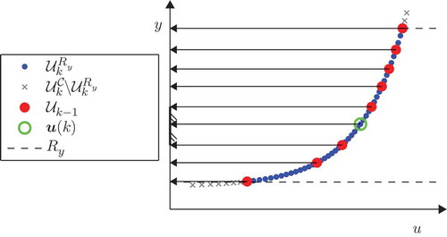
Figure 4. Design point selection using the maximin distance in the input space after the application of eight design points in .

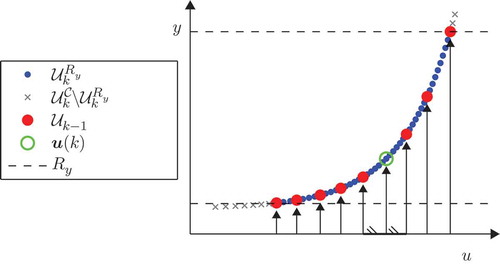
The red dots represent the already applied design points with their observed system outputs . The blue dots represent the design points in with their model output. The crosses represent the design points in that do not have model outputs in .

The adaptation of the MDD consists in selecting iteratively the design point in that have the maximal minimal distance with the already applied design points in (see Figure 4):

(9)

The green circle marks the selected design point which has the maximal minimal distance on the input space (abscissa) to the applied candidates (red dots). If there are several design points for which the maximin distance is equal, these design points are successively applied to the system as the algorithm proceeds. That criterion targets a uniform distribution of applied design points in the input space. Note that, an exactly uniform distribution in the input space is not achieved for every iteration k, but the discrepancy to the uniform distribution is low. This strategy will be termed iCORE DoE.

The drawback of the iCORE DoE is that the choice of the candidate in Equation (9) does not consider the non-linearity of the model in , and thus a strongly non-uniform distribution in the output space results. It points out the resulting disadvantages for non-linear processes, which have locally high output variation to be measured intensively.

3.3.2. Maximin distance on the output space

A second adaptation of the MDD is proposed for the CORE, which profits from the information contained in model for selecting design points, and relies on a distance calculated on the output space. That new criterion targets a uniform distribution of the design points in the output space and corresponds to a strategy termed oCORE DoE (see Figure 5).

Figure 5. Illustration of the oCORE DoE after the application of eight design points in .

In Figure 5, the maximin distance criterion in the output space is illustrated for a one-dimensional input space. The selected design point (green circle) indicates the point of the reduced candidate set (blue dots), which has the maximal minimal distance to the already applied design points (red dots) in the output space (axis of ordinates). The considered distance in the output space is the absolute value of the difference of two outputs:

(10)

The oCORE DoE (10) targets the resulting of a globally uniform distribution at the system output, by limiting iteratively the discrepancy of the observed output distribution with the desired uniform distribution. It selects more design points in areas where a strong variation at the output is observed than the iCORE DoE. However, in the case of a process with ambiguities – different inputs correspond to the same output – Equation (10) does not assure a locally uniform distribution at the system output. Ambiguous output ranges can lead to not uniformly distributed input ranges (see Figure 8(c)).

Figure 6. Illustration of the i/oCORE DoE after the application of eight design points in .

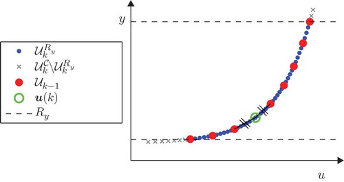
Figure 7. Comparison of model and process after the application of different numbers of design points with the i/oCORE DoE. (a) Three design points. (b) Seven design points.

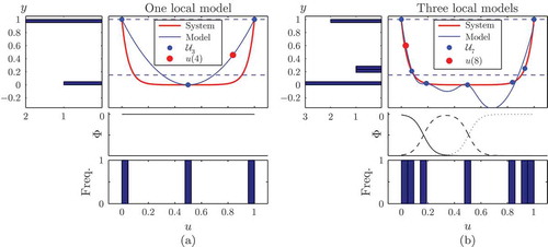
Figure 8. Comparison of model and process after the application of 11 design points with different DoEs. (a) IMDD. (b) iCORE DoE. (c) oCORE DoE. (d) i/oCORE DoE.

3.3.3. Maximin distance on the input/output space

The third criterion proposed for the CORE relies on a distance calculated in the input/output space. It defines a procedure termed i/oCORE DoE, which intends to explore intensively output area with strong variations and avoid unbalanced input distribution. The i/oCORE DoE makes a trade-off between uniform distribution on the input and the output space.

In Figure 6, the maximin distance criterion in the input/output space is illustrated for a one-dimensional input space. The selected design point indicates the point of the reduced candidate set (blue dots), which has the maximal minimal distance in the input/output space to the already applied design points (red dots).

For the computation of the selected design point, the set of all applied design points is augmented by the observed system outputs:

(11)

The selected design point is iteratively determined using the maximin distance calculated on the input/output space. The chosen distance for the design point selection is the extended Euclidean distance:

(12)

An advantage of the i/oCORE DoE is that it selects the design point like the oCORE DoE by exploiting the non-linearity of the model in . But, the i/oCORE DoE is more efficient than the oCORE DoE for systems with ambiguities, since it relies on a trade-off that avoids unbalanced distribution at the system input (see Figure 8(d)).

3.3.4. Criterion properties

Due to the integration of a maximin distance criterion, the iCORE, the oCORE and the i/oCORE DoE are more robust against modelling errors than designs that exclusively depend on a model of the underlying system. For example, D-optimal experimental designs (see [19,20]) are optimal for the identification of systems which are similar to specific models used for the design generation. If there is a discrepancy between the data-based model used for the generation of the DoE and the underlying system, the D-optimal DoE might be insufficient. On the contrary, the three CORE DoEs handle model discrepancies and explore new regions of the input space iteratively by avoiding the repetition of design points. Another advantage is that the three CORE DoEs consider intrinsically output constraints by adjusting to the feasible output range when purely model-based designs consider them afterwards, usually in a constrained optimization.

3.4. Noise consideration in the CORE DoE

For considering the noise in the CORE DoE, two probability densities are used: the estimated ELMN parameter distribution , where is the ELMN parameter vector with length , and the probability density , which describes the output noise and results from the model structure. The restriction to is based on the probability that the observed output is within . If that probability is higher than a threshold value , then the design point is collected in :

(13)

Considering the noise in the CORE DoE (13) should be applied, if the noise is strong compared to .

4. Illustrative example

The three proposed CORE DoEs in combination with an ELMN are demonstrated on a bathtub-like function f, whose output y is given by the maximum of the outputs and of an exponential function and an inverse exponential function , respectively:

(14)

(15)

(16)

The function f has a strong non-linear behaviour in the input ranges 0–0.2 and 0.8–1. In the input interval 0.2–0.8, the function f is almost linear. In this example, is defined by and . For the function f, 19% of the input space is within , where the process model is required to be properly parameterized. This example is justified by qualitatively similar processes that can be found in automotive industry (e.g. and smoke emissions of Diesel engines).

4.1. Illustration of online DoE and modelling

The functionality of the CORE strategy in combination with an ELMN is demonstrated in detail for the i/oCORE DoE. In Figure 7(a), the initial estimation of the ELMN, which is based on a set of three design points , is indicated by the blue line. The initial ELMN consists of one local linear model with a quadratic structure. The red line shows the original process and the blue dashed lines indicate . The blue bars mark the frequency distribution of the design points in the input and in the output space, respectively. The selected design point is given by the red dot.

In Figure 7(b), the process model is shown after the application of seven points. The ELMN consists of three local models, whose validity areas are depicted in the subfigure.

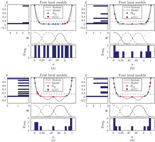
After the application of 11 design points, the identification of the underlying process is stopped. The current ELMN consists of four local models (see Figure 8(d)). Figures 7(a), (b) and 8(d) show that the i/oCORE DoE strategy aims at parameterizing the ELMN systematically in . Six out of eight iterative design points are located in the input space associated with of the real underlying process. This leads to a high frequency distribution and a good approximation of the real process in . Outside of , the frequency distribution is comparably low and the process model shows large deviations from the original process.

4.2. Comparison of design point selection strategies

In order to demonstrate the efficiency of the three CORE DoEs, a comparison with an iterative MDD (IMDD), which does not consider , is given. The results obtained with the IMDD, the iCORE, the oCORE and the i/oCORE DoE are depicted in Figure 8(a)–(d), respectively. The figures present distributions of the selected design points after the application of three initial and eight iterative design points, and depict the model output compared to the unknown actual output of the illustrative example.

The IMDD, which does not considers , ends up with zero iteratively selected design points in (Figure 8(a)). The selected design points divide the design space in iteratively smaller parts: the initial design points are ; the design points and extend the set of applied design points to ; with the design points , the set of applied design points becomes ; finally, the design points and are selected randomly between the previously applied design points. The IMDD leads to an ELMN that outlines the process trend relatively well on the whole design space, but the ELMN is lacking in training data in . The IMDD does not exploit the ELMN, which quality is however sufficient for outlining the input areas which produce training data in .

The iCORE DoE, which in contrary to the IMDD uses the ELMN for selecting design points iteratively, ends up with four design points in (Figure 8(b)). Obviously, the iCORE DoE produces an ELMN with higher model quality in than the IMDD. Note that the model quality outside slightly decreases. The selection of the two first design points is done by the iCORE DoE the same way as the IMDD, since the ELMN estimate initially that those design points produce an output in (see model in Figure 7(a)); But the iCORE DoE continues by selecting different design points, as the ELMN considers that design points in are close to 0 or close to 1. The iCORE DoE does not take the output non-linearity into account for selecting design points, which leads to high distances between the observed outputs, see, e.g., that is selected in an area where the actual output varies less than in an input area closer to 1.

The oCORE DoE, which takes into account the output non-linearity for selecting design points, ends up with six points in (Figure 8(c)). The ELMN quality in is slightly higher for the oCORE DoE than for the iCORE DoE. Note also that the ELMN quality outside is obviously lower for the oCORE DoE. The oCORE DoE, which selects design points by comparing the model output to observed actual outputs, has an approach that is very different to the iCORE DoE. The design points are selected not by considering the input distribution, but for having a model output, between the actually observed outputs (e.g. has a model output between 0 and 1). As a consequence, the selected design points are closer to the input values 0 or 1, compared to the iCORE DoE. The oCORE DoE leads to a global output distribution with a low discrepancy to the uniform distribution (see histogram of Figure 8(c)). The local output distribution is however not uniform: the design point should be placed closer to the input value 0 to achieve a locally more uniform distribution and ascertain high local model quality.

The i/oCORE DoE, which relies on a trade-off for producing design points that are uniformly distributed in the input and in the output space, also ends up with six points in (Figure 8(d)). Note that graphically the model quality after 11 design points with the i/oCORE and the oCORE DoE is similar. It is however possible to notice that the distribution in the output is locally more uniform for the i/oCORE than for the oCORE.

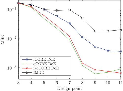
The quality of the ELMNs obtained with the different DoE are quantified using the mean squared errors (MSEs) between the ELMNs and the real underlying process, which are computed with 190 validation data in . In Table 1, the  different MSEs after the application of 11 design points are summarized.

Table 1. Comparison of the number of design points in and the MSE.

Design	Points in	MSE
IMDD	0	193.8
iCORE	4	35.5
oCORE	6	8.98
i/oCORE	6	6.49

The iCORE DoE achieves a more than five times smaller model error than the IMDD. The oCORE DoE and the i/oCORE DoE improve the model quality by four to five times compared to iCORE DoE. The consideration of the output in the maximin distance criteria (10) and (12) explains the additional MSE reduction.

For comparing the oCORE and the i/oCORE DoE, an analysis of the model quality according to the number of design points is done (see Figure 9). The three CORE DoEs may give no unique solution for the design point selection. In this case, the proposed algorithm iteratively chooses one of all possible design points. Since the considered function is symmetric around , there is no unique assignment of any output to an input. Therefore, oCORE DoE results in a non-uniform distribution of design points in the left and right domain of . The overall frequency distribution at the output is very uniform, but the oCORE DoE leads to locally non-uniform frequency distributions at the output for functions with ambiguities. The quality of the ELMN is increased in areas where a higher design point density is reached, but that is overcompensated by a decrease of the model quality in areas of lower design point density. This effect causes for this example a slight increase of the MSE for the oCORE DoE when the number of design points is increased from 9 to 11.

Figure 9. Evolution of the MSE of the ELMNs. Best results are achieved for i/oCORE DoE.

The three CORE DoEs are efficient methods that systematically parametrize the process model in for the design space exploration. This results in a higher model quality in in comparison with a standard IMDD with an equal number of design points. Alternatively speaking, the CORE DoE achieves the same model quality with less experimental effort compared to the IMDD.

5. Application examples

The CORE DoE strategy is applied to two typical application examples for Diesel engine calibration. In the following, the three CORE DoEs are used for the identification of a and a smoke model of a Diesel engine. Since emission norms are continuously tightened, proper models are required for the optimization of the engine control unit (ECU), so that legislative emission norms are satisfied. Engine test bed experiments are very expensive and therefore an efficient parametrization is very much desired in industry.

5.1. modelling

During the combustion, formation is described under most of the conditions by the thermal Zeldovitch mechanism, but also a not well-understood part of the emission is due to the prompt Fenimore and mechanisms (see [21]). The internal engine quantities that influence these mechanisms are, e.g., the cylinder pressure, the gas temperature and flow, and the exhaust gas recirculation (EGR) (see [22]).

In this section, the process is a physical model of a 6-cylinder Diesel combustion engine developed in the software environment BOOST CS (AVL List GmbH, Graz, Austria; see [23]). The engine components are simulated using the finite difference method. The internal engine quantities, which may influence the emissions, are controlled by an ECU. The pedal position (load signal) and the engine speed are here kept constant during the combustion engine simulation and define the operating point. In this paper, attention is given to the following operating point:

• engine speed: 1500 rpm

• load signal: 0.3

All the internal engine quantities are initialized with plausible values and vary during the simulation. They however converge over time to a cyclostationary (or stationary) state. In this paper, the effects of three internal engine quantities on the emission are analysed around the chosen operating point. For that purpose, three internal quantities are set free from the ECU and are instead actuated in the following ranges:

• swirl position: 0–0.7

• EGR rate: 0–0.27

• rail pressure: 300–800 bar

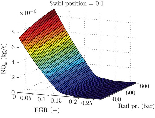
Figure 10 shows the intersection plot of the emission estimated by an ELMN, when the EGR and the rail pressure vary and the swirl position is constant. The emission estimation behaves the characteristic way of a Diesel engine; the emission decreases when the EGR is increasingly opened (see [24]).

Figure 10. Illustration of emission for a Diesel engine model.

5.1.1. CORE DoE

For this example, it is intended to explore () where the quality of the ELMN must be high. An initial central composite design (CCD) with additional intermediate design points (see [16]) consisting of 15 design points is generated for the estimation of the initial ELMN. CCDs are commonly used for fitting second-order models (see [25]). A design point corresponds to a swirl position, an EGR opening rate and a rail pressure that are the only varying system inputs. Figure 11(a) shows the distribution of the observed emissions obtained with the design points of the initial design. The abscissa represents samples corresponding to the three-dimensional design points of the initial DoE. The sample numbers of the design points are ordered by growing emissions.

Figure 11. Comparison of emission distributions obtained with the initial and the iterative designs. (a) Initial design. (b) CORE and standard DoE.

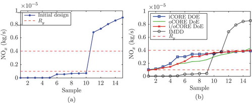
The observed emissions with the initial design cover the range 0–0.9 (), which is significantly wider as . Note moreover that Figure 11(a) shows no observation within .

After the initial DoE, 15 design points are iteratively applied using the iCORE, the oCORE and the i/oCORE DoE, and a comparison is done with the IMDD. As depicted in Figure 11(b), for the three CORE DoEs, most of the observations are within , which shows that the ELMNs estimate suitably the relations between the inputs and the output of the systems. Note that the oCORE DoE produce one emission slightly outside of , which is due to the slight imprecisions of the ELMN. In comparison, the IMDD sets only two design points that produce emissions in .

5.1.2. Model quality

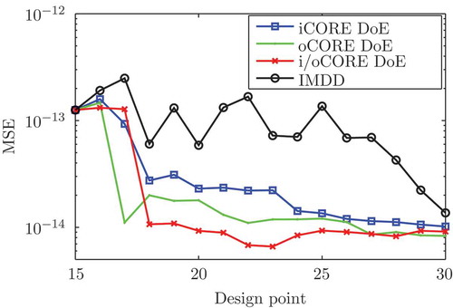
In Figure 12, the model quality as a function of the applied design points is depicted for the IMDD, as well as for the iCORE, the oCORE and the i/oCORE DoE. The validation data are produced with simulations of the physical engine model, generated with a full factorial DoE. It is the 28 samples with an output in that are used to calculate the MSE. A qualitatively similar result to Figure 9 is obtained. The three CORE DoEs show a significant reduction of the MSE compared to the standard IMDD, but the iCORE DoE has a higher MSE compared to the i/oCORE and the oCORE DoE. Since the i/oCORE DoE assures a locally uniform output distribution, it is preferable to the oCORE DoE.

Figure 12. Evolution of the MSE of the ELMNs with the standard and the CORE designs.

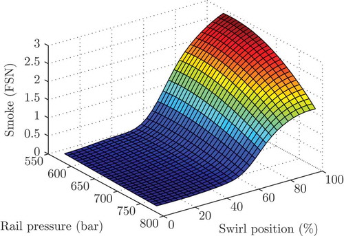
5.2. Smoke modelling

Smoke denotes particles in the exhaust of Diesel engines mainly consisting of not combusted carbon compounds. Smoke emissions are influenced by the temperature and the ratio of air to fuel in the combustion chamber (see [24]). The smoke concentration in the exhaust is determined in the unit of filter smoke number (FSN). In this example, test bed data of a real Diesel engine are used to obtain an accurate smoke reference model for the evaluation of the CORE DoE strategy. This model is based on 1796 uniformly distributed measurements in a five-dimensional input space. The obtained model properly approximates the smoke emissions of the underlying engine. For smoke modelling, the following input channels are used:

• rail pressure

• timing of main injection

• timing of pilot injection

• swirl position

• EGR rate

In Figure 13, an intersection plot of the smoke model as a function of swirl position and rail pressure is depicted. The smoke emission is typically increased when the swirl position exceeds a certain threshold value. This application example is presented for demonstrating that the i/oCORE DoE achieves a significant improvement in the model quality, even when noise at the system output is present.

Figure 13. Intersection plot of smoke as function of swirl position and rail pressure.

5.2.1. CORE DoE

For this example, it is required that the smoke model has a high model quality for FSN higher than (). The initial DoE for the estimation of the initial ELMN is also based on a CCD with additional intermediate design points. The initial DoE consists of 85 design points. In Figure 14(a), the sorted output obtained by the initial DoE is depicted. Only 24% of the data are within , which already indicates that there is great potential for input space reduction by the CORE DoE strategy.

Figure 14. Comparison of soot emission distributions obtained with the initial and the i/oCORE DoE. (a) Initial design. (b) i/oCORE DoE.

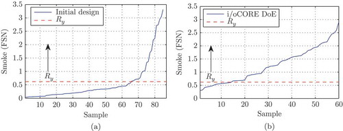
The iterative DoE is here an i/oCORE DoE that consists of 60 design points. In Figure 14(b), the ordered system output is depicted. The design points are nearly uniformly distributed in the output space and the output prediction of the ELMN is for most of the design points in of FSN higher than .

5.2.2. Model quality

In total, 100 ELMNs are trained in order to obtain a statistically reliable result for the model quality (Monte Carlo simulation). For each training data set, noise is added at the output. The obtained models are evaluated with 1000 randomly generated validation points in . The output of the validation points is obtained from the accurate reference model. In Figure 15(b), the root of the mean squared error (RMSE) as a function of the sample size is depicted for the i/oCORE DoE.

Figure 15. Evolution of the model error with the total number of applied design points. A stronger error reduction is achieved with the CORE DoE than with the standard IMDD. (a) IMDD. (b) i/oCORE DoE.

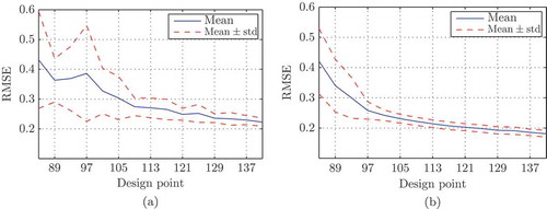
In Figure 15(a), the RMSE is shown for the IMDD. The mean of the model error of the i/oCORE DoE is reduced by about and the standard deviation is also considerably smaller compared to the standard IMDD.

6. Conclusion

In the present paper, an online methodology for the efficient parametrization of non-linear stationary models in a custom range of the system output is presented. The proposed CORE DoE strategy uses the prediction of an ELMN in order to improve the model quality in a , where high accuracy is required. The selection of the design points in is based on a distance criterion, which can be applied in the input, the output and in the combined input/output space.

The CORE DoE concept is based on a trade-off between model exploitation and space exploration that is robust against inaccuracies of the ELMN and avoids the repetition of design points. The generation of new design points is not based on convex optimization, but on a selection of design points in a finite set. Therefore, the CORE DoE concept is applicable to processes with a non-convex response. The CORE DoE is intrinsically conceived for system identification in the presence of system output constraints. The functionality and efficiency of the systematic model parametrization in is demonstrated on an illustrative example. The analysis of the model error demonstrates that the i/oCORE DoE achieves very promising results.

The three CORE DoEs are applied for a typical automotive identification task of a emission model. For this purpose, the CORE DoE methodology is validated on a Diesel engine represented by a complex simulation tool based on physical modelling. The achieved model quality of the CORE DoE is superior to the standard IMDD. Moreover, the i/oCORE DoE is tested in a Monte Carlo simulation with noise at the system output in order to identify a smoke model with a five-dimensional input space. In this case, the original process is represented by an accurate reference model based on real test bed data of a Diesel engine. This application example also confirms that the model quality is significantly enhanced with the CORE DoE compared to the standard IMDD.

The CORE presents a promising contribution to industries where data-driven modelling is common, e.g. the automotive, the aerospace or the medical industry. Those industries often design experiments for modelling processes that are of interest within custom output ranges, e.g. prescribed ranges of physiological values or combustion product quantities or quality. The CORE offers to those industries a methodology reducing the experimental effort compared to standard techniques, by producing models with high quality in custom output ranges with less experimental runs.

Acknowledgement

This work was supported by the Christian Doppler Research Association and AVL List GmbH.

References

- C. Hametner, M. Stadlbauer, M. Deregnaucourt, and S. Jakubek, Incremental optimal process excitation for online system identification based on evolving local model networks, Math. Comput. Model. Dyn. Syst. 19 (13) (2013), pp. 505–525. doi:10.1080/13873954.2013.800122.
- P. Ranjan, D. Bingham, and G. Michailidis, Sequential experiment design for contour estimation from complex computer codes, Technometrics. 50 (2008), pp. 527–541. doi:10.1198/004017008000000541.
- E. Vazquez and J. Bect, A sequential Bayesian algorithm to estimate a probability of failure, Proceedings of the 15th IFAC Symposium on System Identification, SYSID 2009, Saint-Malo, July 2009, p. 5.
- H. Arenbeck, S. Missoum, A. Basudhar, and P. Nikravesh, Reliability-based optimal design and tolerancing for multibody systems using explicit design space decomposition, J. Mech. Des. 132 (2010), p. 021010. doi:10.1115/1.4000760.
- V. Picheny, D. Ginsbourger, O. Roustant, R.T. Haftka, and N.H. Kim, Adaptive designs of experiments for accurate approximation of a target region, J. Mech. Des. 132 (2010), p. 071008. doi:10.1115/1.4001873.
- R.C. Kuczera and Z.P. Mourelatos, On estimating the reliability of multiple failure region problems using approximate metamodels, J. Mech. Des. 131 (2009), p. 121003. doi:10.1115/1.4000326.
- E. Lughofer, FLEXFIS: A robust incremental learning approach for evolving Takagi–Sugeno fuzzy models, IEEE Trans. Fuzzy Syst. 16 (2008), pp. 1393–1410. doi:10.1109/TFUZZ.2008.925908.
- O. Nelles, Nonlinear System Identification: From Classical Approaches to Neural Networks and Fuzzy Models, Springer, Berlin, 2001.
- C. Hametner and S. Jakubek, Engine model identification using local model networks in comparison with a multilayer perceptron network, Proceedings of the 2nd International Multi-Conference on Complexity, Informatics and Cybernetics: IMCIC, Orlando, FL, March 2011.
- B. Hartmann, J. Moll, O. Nelles, and C.P. Fritzen, Hierarchical local model trees for design of experiments in the framework of ultrasonic structural health monitoring, IEEE International Conference on Control Applications (CCA), Denver, CO, September 2011, pp. 1163–1170.
- C. Hametner and S. Jakubek, Local model network identification for online engine modelling, Inf. Sci. 220 (2013), pp. 210–225. Online Fuzzy Machine Learning and Data Mining. doi:10.1016/j.ins.2011.12.034.
- M. Johnson, L. Moore, and D. Ylvisaker, Minimax and maximin distance designs, J. Stat. Plann. Infer. 26 (1990), pp. 131–148. doi:10.1016/0378-3758(90)90122-B.
- E. Stinstra, D. den Hertog, P. Stehouwer, and A. Vestjens, Constrained maximin designs for computer experiments, Technometrics. 45 (2003), pp. 340–346. doi:10.1198/004017003000000168.
- O. Nelles, Nonlinear System Identification, 1st ed., Springer-Verlag, Berlin Heidelberg, 2002.
- P. Pucar and M. Millnert, Smooth hinging hyperplanes – An alternative to neural networks, Proceedings of the 3rd ECC, Rome, September 1995.
- L. Eriksson, Design of Experiments: Principles and Applications, Umetrics Academy, Umeå, 2008.
- Y. Bard, Nonlinear Parameter Estimation, Academic Press, New York, 1973.
- T. Santner, B.J. Williams, and W. Notz, The Design and Analysis of Computer Experiments, Springer Series in Statistics, Springer, New York, 2003.
- L. Pronzato, Optimal experimental design and some related control problems, Automatica. 44 (2008), pp. 303–325. doi:10.1016/j.automatica.2007.05.016.
- G. Franceschini and S. Macchietto, Model-based design of experiments for parameter precision: State of the art, Chem. Eng. Sci. 63 (2008), pp. 4846–4872. doi:10.1016/j.ces.2007.11.034.
- C.J. Mueller, A.L. Boehman, and G.C. Martin, An experimental investigation of the origin of increased NOx emissions when fueling a heavy-duty compression-ignition engine with soy biodiesel, SAE Int. J. Fuels Lubr. 2 (2009), pp. 789–816.
- C. Ericson, B. Westerberg, M. Andersson, and R. Egnell, Modelling diesel engine combustion and NOx formation for model based control and simulation of engine and exhaust aftertreatment systems, SAE Paper, 2006, pp. 01–0687. doi:10.4271/2006-01-0687.
- J.C. Wurzenberger, R. Heinzle, A. Schuemie, and T. Katrasnik, Crank-Angle Resolved Real-Time Engine Simulation – Integrated Simulation Tool Chain from Office to Testbed, SAE International, Warrandale, PA, 2009.
- R. Basshuysen and F. Schaefer (eds.), Handbuch Verbrennungsmotor, Vieweg, Braunschweig, 2002.
- R.H. Myers, D.C. Montgomery, and C.M. Anderson-Cook, Response Surface Methodology: Process and Product Optimization Using Designed Experiments, 3rd ed., Wiley Series in Probability and Statistics, Wiley, Hoboken, NJ, 2009.